HAL Id: hal-00852866
https://hal.archives-ouvertes.fr/hal-00852866
Submitted on 21 Aug 2013
HAL is a multi-disciplinary open access
archive for the deposit and dissemination of
sci-entific research documents, whether they are
pub-lished or not. The documents may come from
teaching and research institutions in France or
abroad, or from public or private research centers.
L’archive ouverte pluridisciplinaire HAL, est
destinée au dépôt et à la diffusion de documents
scientifiques de niveau recherche, publiés ou non,
émanant des établissements d’enseignement et de
recherche français ou étrangers, des laboratoires
publics ou privés.
Evaluating Structural Pattern Recognition for
Handwritten Math via Primitive Label Graphs
Richard Zanibbi, Harold Mouchère, Christian Viard-Gaudin
To cite this version:
Richard Zanibbi, Harold Mouchère, Christian Viard-Gaudin. Evaluating Structural Pattern
Recog-nition for Handwritten Math via Primitive Label Graphs. Document RecogRecog-nition and Retrieval XX,
Feb 2013, Burlingame, United States. pp.865817-865817-11, �10.1117/12.2008409�. �hal-00852866�
Evaluating Structural Pattern Recognition
for Handwritten Math via Primitive Label Graphs
Richard Zanibbi
a, Harold Mouch`
ere
band Christian Viard-Gaudin
ba
Dept. Computer Science, Rochester Institute of Technology,
1 Lomb Memorial Drive, Rochester, NY, USA
b
L’UNAM/IRCCyN/Universit´
e de Nantes,
rue Christian Pauc, 44306 Nantes, France
ABSTRACT
Currently, structural pattern recognizer evaluations compare graphs of detected structure to target structures (i.e. ground truth) using recognition rates, recall and precision for object segmentation, classification and relationships. In document recognition, these target objects (e.g. symbols) are frequently comprised of multiple primitives (e.g. connected components, or strokes for online handwritten data), but current metrics do not characterize errors at the primitive level, from which object-level structure is obtained. Primitive label graphs are directed graphs defined over primitives and primitive pairs. We define new metrics obtained by Hamming distances over label graphs, which allow classification, segmentation and parsing errors to be characterized separately, or using a single measure. Recall and precision for detected objects may also be computed directly from label graphs. We illustrate the new metrics by comparing a new primitive-level evaluation to the symbol-level evaluation performed for the CROHME 2012 handwritten math recognition competition. A Python-based set of utilities for evaluating, visualizing and translating label graphs is publicly available.
Keywords: Evaluation, Performance Metrics, Structural Pattern Recognition, Math Recognition, Graphics Recognition
1. INTRODUCTION
In this paper we are interested in evaluating structural pattern recognition, i.e. where the output is some form of graph over primitives provided in data files. Examples of common primitives include connected components in images, or handwritten strokes collected using a tablet. We will use handwritten mathematical expression recognition from pen/finger strokes for illustration.1, 2
Structure can be evaluated at three different levels of abstraction: the symbolic, object, and primitive. The symbolic level is most abstract, and does not consider input primitives at all. It represents only objects types and object relationships. Comparing text from an OCR system to ground truth by Levenshtein distance or longest common sub-sequences3 is an example of a symbolic-level comparison. Another example is comparing handwritten math expressions using LATEX strings, which represent only symbol identities and their relationships, and not which strokes belong to each symbol. At the object level, objects are defined by a partition of the primitives, such as handwritten strokes grouped into symbols. Objects have associated types and relationships, the same used in a symbolic level representation. The lowest level of abstraction is the primitive level, where we consider every primitive in the input, e.g. every stroke in a handwritten expression and relationships between primitives. An advantage of the primitive level is that the smallest units of comparison are shared by recognition outputs and ground truth. As a result, there are not the types of correspondence issues that evaluating outputs at the object and symbolic levels often involve (due to over/under-segmentation, for example). As we will illustrate, with an appropriate primitive representation, object and symbolic-level representations may also be obtained.
Further author information: R.Z.: [email protected]
H.M.: [email protected] C.V.G.: [email protected]
Table 1: CROHME Part III Dataset Statistics Expressions Symbols Strokes Train 1336 16946 24731
Test 486 6381 8832
Our primitive structure representation (label graphs) and metrics were devised with two goals in mind: 1) characterize errors in classification, segmentation, and parsing, and 2) be useful for retrieving structural patterns. Satisfying 1) allows machine learning algorithms to be created that minimize global cost functions characterizing overall accuracy of complete structure graphs. We will use the domain of online mathematical expression recognition for examples, and the recent CROHME competition4to illustrate the proposed method. However, as suggested in the extension section, the method is very general, and can be adapted to other domains, and also to multiple levels of structure, e.g. when mathematics contains matrices, that in turn contain sub-expressions. Label graphs have also been use for retrieving mathematical expressions represented in LATEX (i.e. using label graphs to represent structure, but at the symbolic level).5
The key idea in our approach is to attach all results obtained in different processing stages, namely segmenta-tion, recognition and parsing (structural analysis) to the primitives in the input document. Structure is described by a directed graph over the set of primitives. Primitives are represented by nodes, and edges between primitives identify segmentation and relationships between objects such as spatial relationships or syntax relationships (e.g. identifying the arguments of an operator in a mathematical expression).
In the next Section we introduce the CROHME competition and its evaluation protocol (Section 2). In Section 3 we define our label graph representation, introduce Hamming distance-based metrics over label graphs, relate our metrics to existing metrics, and describe a publicly available set of tools for computing our metrics and visualizing structure. In Section 4 we apply these tools to the CROHME 2012 output data, and discuss the results obtained. We describe extensions and other applications of our metrics in Section 5, and then conclude in Section 6.
2. THE CROHME HANDWRITTEN MATH RECOGNITION COMPETITION
The CROHME competition (Competition on Recognition of On-line Mathematical Expressions) has been run twice to date, in 20116and 2012.4 Expressions used in CROHME are represented using an extension of the W3C InkML standard. CROHME training data files contains three elements: 1) a sequence of (x,y) coordinates for each stroke, 2) symbol level ground truth, containing a partition of stroke identifiers into symbols, and a symbol class for each symbol, and 3) the ground truth structure encoding, representing symbol layout in Presentation MathML∗, with annotations making reference to symbols (stroke sets). Ground truth was created manually. An important restriction is that all strokes belong to exactly one symbol in an expression.
In the 2012 competition, systems were evaluated using three progressively more complex expression languages, defined by context-free grammars for a subset of LATEX math strings. The number of symbol classes and allowable relationships between symbols increases with the difficulty level. We focus on the most difficult expression set, referred to as “part III.” Table 1 presents some statistics for the part III training and test sets.† There are 75 symbol classes, including digits, Latin and Greek letters, arithmetic operators, and other symbols. Common spatial relationships and structures are permitted: sub-scripts, super-scripts, fractions, square roots, limits, summations, etc. These are few limitations on recursive structure in part III. Vectors, matrices and other tabular structures are not included. Participants were provided with training data, and then had their systems tested by the organizers using a separate test set. Systems needed to produce InkML files in the same format used for the training data.
As the evaluation script compares structure through exact matching of MathML strings, MathML in system outputs need to use the same format as ground-truth. Unfortunately, several valid MathML structures may
∗
InkML: http://www.w3.org/TR/InkML/, MathML: http://www.w3.org/Math/
†
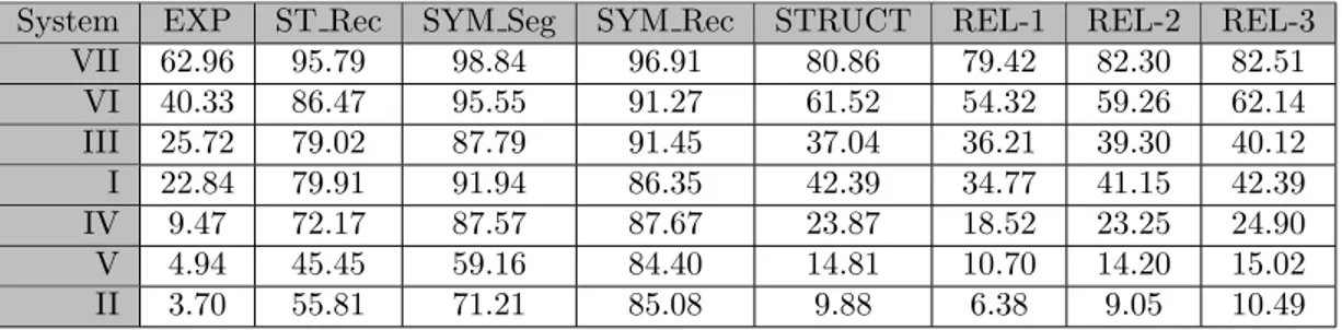
Table 2: CROHME 2012 Part III Metrics (%) for Submitted Systems.4 Participants are sorted by expression rate (EXP)
System EXP ST Rec SYM Seg SYM Rec STRUCT REL-1 REL-2 REL-3 VII 62.96 95.79 98.84 96.91 80.86 79.42 82.30 82.51 VI 40.33 86.47 95.55 91.27 61.52 54.32 59.26 62.14 III 25.72 79.02 87.79 91.45 37.04 36.21 39.30 40.12 I 22.84 79.91 91.94 86.35 42.39 34.77 41.15 42.39 IV 9.47 72.17 87.57 87.67 23.87 18.52 23.25 24.90 V 4.94 45.45 59.16 84.40 14.81 10.70 14.20 15.02 II 3.70 55.81 71.21 85.08 9.88 6.38 9.05 10.49
represent the same expression, and so a normalized encoding is defined. MathML formatting rules are checked in the evaluation program made available to participants, generating warning messages when appropriate. To help participants, some graph transformation operations are performed to normalize structure, such as requiring MROW tags for horizontally adjacency symbols to have at most two children, with a right recursive structure for longer sequences of adjacent symbols.
In CROHME 2012, systems were evaluated using the metrics below. The STRUCT and REL-* metrics are at the symbolic level of comparison described earlier. ST Rec is a primitive level metric, while the remaining metrics are defined at the object level (i.e. symbol level).
(i) EXP: the percentage of expressions with correctly recognized symbols and structure. This is challenging, as an expression with any symbol or layout error is considered incorrect.
(ii) ST Rec: the stroke classification rate, the percentage of strokes with the correct symbol label,
(iii) SYM Seg: the symbol segmentation rate (i.e. symbol recall), the percentage of correctly segmented symbols in ground truth,
(iv) SYM Rec: the symbol recognition rate for correctly segmented symbols
(v) STRUCT: the percentage of expressions with correct layout relationships between symbols in the MathML output. This ignores symbol segmentation and classification, requiring only that some symbol appear at the correct positions for symbols in the symbol layout tree (see Figure 1(d)). For example, “2 + 2” and “i = 9” share the same symbol layout tree, as do “x2− 1” and “2a+ b”.
(vi) REL-1/-2/-3, the percentage of expressions correctly recognized with 1, 2 or 3 errors in symbol class or MathML layout tags, e.g. MSUP vs. MROW used to indicate superscript vs. horizontal adjacency, for trees with a layout structure matching ground truth. Note that these values may be both lower and higher than STRUCT, because symbol classes are ignored in STRUCT, and some incorrect spatial relationships leading to an expression not being counted in STRUCT may be repaired. No attempt is made to restructure trees, only to relabel nodes in the MathML symbol layout representation.
Training and test data, a syntax validator and evaluation tools are publicly available from the International Association of Pattern Recognition (IAPR).‡ Most output files from participants are also available. Table 2 shows the results for each participant with the CROHME measurements.4
‡
http://www.iapr-tc11.org/mediawiki/index.php/CROHME:_Competition_on_Recognition_of_Online_ Handwritten_Mathematical_Expressions
3. STRUCTURE MATRICES AND EVALUATION METRICS
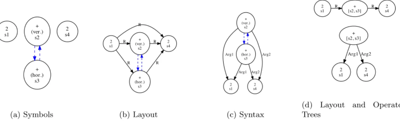
We now define label graphs along with metrics for evaluating structure recognition at the primitive level. Es-sentially, label graphs are directed graphs over primitives, which we represent using adjacency matrices. In a label graph, nodes represent primitives, while edges define primitive segmentation (i.e. ‘merge’ relationships) and object relationships. Figure 1(a) shows a directed graph representing symbols (objects) for a handwritten “2+2”. Two strokes belong to the symbol “+”, and one stroke for each of the “2” symbols, giving three objects for four input primitives. In our representation relationships are defined at the level of objects, implying that all primitives in a symbol have the same incoming and outgoing edges.
Figures 1(b) and (c) show different representations for a handwritten “2+2” based on symbol layout and operator syntax. Figure 1(a) represents symbol layout, showing that left-to-right we have “2” followed by a “+” and then another “2”. Figure 1(c) represents the mathematical syntax of the expression, with “+” as a binary operator with two arguments. Figure 1(d) shows 1(b) as a symbol layout tree and (c) as an operator tree, where nodes represent symbols. Layout trees are roughly equivalent to LATEX and Presentation MathML, and operator trees to Content MathML and abstract expression syntax used in programming language compilers. Both have been used for math recognition and retrieval, and layout trees may be mapped to operator trees.7
2 s1 + (ver.) s2 + (hor.) s3 2 s4 (a) Symbols 2 s1 + (ver.) s2 R 2 s4 R + (hor.) s3 R R R (b) Layout + (ver.) s2 + (hor.) s3 2 s1 Arg1 2 s4 Arg2 Arg1 Arg2 (c) Syntax 2 s1 + [s2, s3] R 2 s4 R + [s2, s3] 2 s1 Arg1 2 s4 Arg2
(d) Layout and Operator Trees
Figure 1: “2+2” Written Using Four Strokes. (a)-(c) are primitive label graphs, and (d) shows trees over objects (symbols) whose structure are equivalent to (b) and (c). Strokes are named in writing order as s1, s2, s3 and s4 with the vertical and horizontal strokes for the ’+’ indicated by (ver.) and (hor.). Dashed edges indicate strokes merged into a symbol. Nodes are labeled with the class of the symbol associated with a stroke. Remaining edges represent relationships: R for adjacent-at-right, and Arg1 and Arg2 for operator arguments
In Figure 1(b), the relationship between the rightmost “2” and the leftmost “2” is due to the “R” (adjacent-at-right) and other spatial relationships being hierarchical in our representation. For example, for the LATEX ex-pression 2^{x-1}, “x”, “-”, and “1” are in the superscript region of “2”, not just the “x”, and both the “-” and “1” are adjacent to the “x”. If a system returns “2_{x}^{-1}” for this expression, the subscript with x is incorrect, and there is a missing adjacency between “x” and “-”; but the detected superscript containing “-1” is correct, and we capture this using this representation.8
For evaluation, we represent our labeled directed graphs over primitives using label graphs. Figure 2(a) visualizes these as adjacency matrices of labels: the diagonal provides primitive labels and other cells provide primitive pair (edge) labels. Figures 2(b) to 2(d) are label graphs for the graphs in Figure 1, with the label graph format shown first. To ease comparison, we use “1” and “2” to represent “Arg1” and “Arg2” in the syntax graph. The underscore (’ ’) identifies unlabeled primitives and relationships (e.g. ’no relationship’), and an asterisk (’*’) represents two primitives in the same symbol.
Relative to Figure 1(a), some relationships in Figures 1(b) and (c) differ. The matrices differ where new relationships add edges to the graph. For n primitives (e.g. strokes), there are n2labels in a primitive structure graph (16 labels for Figures 1(a)-(c)). For C object classes (i.e. possible primitive labels), and L relationship types, the number of possible primitive structure graphs is CnLn(n−1). For C = 100 symbol classes and L=10
s1 l1 e12 e13 e14 s2 e21 l2 e23 e24 s3 e31 e32 l3 e34 s4 e41 e42 e43 l4
(a) Format
2
+ * * +
2 (b) from Fig. 1(a)
2 R R R + * R * + R 2 (c) from Fig. 1(b) 2 1 + * 2 2 * + 2 2 (d) from Fig. 1(c)
Figure 2: Adjacency Matrices for Label Graphs. Figure (a) shows the adjacency matrix format (li for the label of primitive i and eij of the label of the edge from primitive i to j). Figures (b) to (d) show matrices for Figure 1
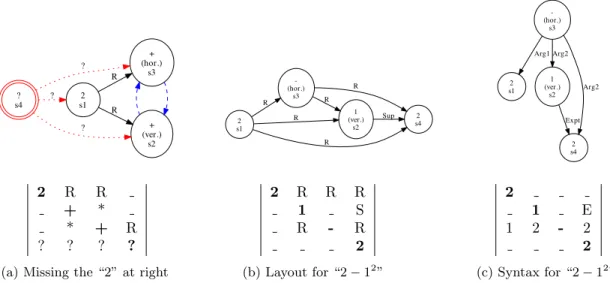
2 s1 + (ver.) s2 R + (hor.) s3 R ? s4 ? ? ? 2 R R + * * + R ? ? ? ? (a) Missing the “2” at right
2 s1 -(hor.) s3 R 1 (ver.) s2 R 2 s4 R R R Sup 2 R R R 1 S R - R 2 (b) Layout for “2 − 12” 2 s1 1 (ver.) s2 2 s4 Expt -(hor.) s3 Arg1 Arg2 Arg2 2 1 E 1 2 - 2 2 (c) Syntax for “2 − 12”
Figure 3: Different Interpretations for “2+2” in Fig. 1. In (a) we have recognized “2+” and compare this with Figure 1(b). The missing stroke in the interpretation is treated as unrelated to strokes present in the expression, with an undefined label and undefined relationships with other strokes. In (b) the ’+’ is split, with a superscript between strokes s2 and s4. In (c) the exponent “12” is represented by the edge labeled “Expt.”
available relationships between symbols, the set of possible interpretations is 1020 for four strokes. Many of these are illegal, as when primitives in an object have different relationships with other primitives. However, hundreds of math symbols are in use. Also, for symbol layout we need to represent primitives in the same symbol (the dashed edges in Figure 1) along with spatial relationships, so the sizes for C and L are realistic. For mathematical notation, common spatial relationships include above, below, adjacent-at-right, superscript, subscript, left-superscript, left-subscript, contained (e.g. by square root), and no relationship.9
3.1 Representing Missing Primitives
We can account for primitives that are in one but not another label graph. This is important when a recognition system produces only partial output, such as seen in the CROHME competition (see Section 4). In Figure 3(a), we see the result of comparing just the first three strokes in Figure 1(a) (“2+”) to the full expression (“2+2”). We obtain the set of primitive identifiers for both label graphs, and then produce a label graph for the complete primitive set. For missing primitives, we use a distinct absent (“?”) label for the primitive and all its edges. All relationships from primitives in the interpretation to absent/missing primitives are treated as no relationship (“ ”), as none were created in producing the interpretation.
Figure 3(a) differs from Figure 1(a) by one primitive label (“?” vs. “2”), and five relationships, for a total difference of six labels. In the case where two interpretations have primitives not provided in the other interpretation, we repeat the process described above, defining every missing primitive from either graph as absent (“?”), and adding absent relationships from the absent primitive to all other primitives present in both graphs.
3.2 Metrics for Label Graphs
Structure errors over a set of primitives are simply the locations where two label graphs differ. The Hamming distances of interest between two label graphs are:
1. ∆C, the number of primitive labels that differ
2. ∆L = ∆S + ∆R, the number of directed primitive pair edges that differ. This represents segmentation errors by the number of incorrect merges/splits between primitive pairs (∆S), along with additional object relationship errors represented at the primitive level (∆R)
3. ∆B = ∆C + ∆L = ∆C + ∆S + ∆R, the Hamming distance between the adjacency matrices
For illustration, in Figure 3(b) we show an incorrect interpretation of our handwritten “2+2” where we split the two strokes in the “+” and obtain “2 − 12”. In the syntax representation (Figure 3(c)) edges identify which primitives belong to arguments of explicit operators such as ”+” (e.g. ”Arg1,” ”Arg2”), and also implicit binary operations (e.g. exponent or subscripts representing indices). The“Expt” edge has its tail connected to all primitives belonging to the base of the exponent, and the head connected to all primitives in the exponent - the label itself identifies that exponentiation is the operator to be applied. In Figure 3(c), we apply the exponent before performing subtraction.
Consider differences in the label graphs for layout and content in Figures 2(b) and (c). Splitting the “+” leads to a ∆C of two for the new layout and expression syntax interpretations when comparing Figures 3(b) and (c) to Figures 1(b) and (c), with “+” has been replaced by “1” and “-”. ∆S is also two, as the two strokes in “+” have been split apart (i.e. the two ‘*’ have been removed, replaced by ’ ’ and ’R’ in Figure 3(b), and ‘ ’ and ‘Arg2’ in Figure 3(c)). The number of differing relationships (∆L) are three for the layout trees (∆S = 2; plus new superscript relationship, so ∆R = 1) and five for the syntax trees (∆S = 2, plus ∆R = 3). The total Hamming distance (∆B = ∆C + ∆L) for the label graphs are five for layout, and seven for expression syntax.
We define two additional metrics for evaluation at the level of complete structure graphs: 1. ∆Bn= ∆Bn2 , the percentage of correct label graph labels
2. ∆E = ∆C n + p ∆S n(n−1)+ p ∆L n(n−1)
3 , errors averaged over classification, segmentation and all relationships For n input primitives, ∆Bn is the Hamming distance normalized by the label graph length, converting ∆B to a percentage. ∆E is an average error per-primitive, for classification, segmentation, and all primitive pair relationships. As ∆S is part of ∆L, segmentation errors are emphasized more than other edge label/relationship errors (∆R) in the metric. Note if n = 1, ∆L and ∆S are 0, as there are no edges in the graph, and in that instance one computes ∆C/n.
3.3 Implementation
The authors have developed tools implemented in Python to support creating, comparing, visualizing and trans-lating label graphs to other formats§. These tools were used to produce the CROHME results provided in the next Section. Included is a Perl utility for converting CROHME InkML data to label graphs, along with a tool to generate LATEX and other string encodings from graph files. GraphViz (.dot) output for bipartite, directed graph, and structure tree outputs may also be produced (as seen in Figures 1 and 3). Graphs representing object structure (segments) and disagreements between graphs can also be produced automatically.
Graphs and evaluation metrics are stored in simple comma-separated variable (CSV) and text files. Com-paring graph files produces a pair of files, one containing evaluation metrics (.m, a list of metric name/value pairs), and a second containing the differences between label graphs (.diff). Each node and edge is annotated with a label and confidence value. Currently we do not use confidences, but node/edge labels may have a set of unique labels with associated confidence values, provided using multiple node or edge entries in a CSV graph file. Reported metrics include recall and precision measures for objects and object relationships (e.g. symbols, and spatial relationships between symbols), which are computed directly from label graphs.
§
3.4 Comparing Metrics for Primitive, Object and Symbolic Representations
The primitive-level Hamming-distance metrics (∆C, ∆L, ∆S, and ∆B) quantify the number of decisions over primitives that differ between interpretations, providing uniform, absolute measures of error at the primitive level. In computing these, we can determine precisely which and how many primitive and primitive pair labelings are incorrect, exploiting the direct correspondence between primitives in the structure graphs begin compared. However, the number of primitive pair errors for segmentation and relationships/structure are sensitive to the size of objects involved. For example, as the number of primitives in an object increases, the cost of splitting away a single primitive also increases, because a proper segmentation requires all primitives in the object to be related by a ‘*’ (merge) relationship. As a result, our Hamming distance measures complement rather than replace object-level metrics, with each characterizing errors at a different level of abstraction. To mitigate the multiplicative effect of large objects on structural error counts, ∆E weights classification, segmentation and spatial relationship edges roughly equally within an expression (see earlier discussion).
At the object-level, segmentation errors are identified by mismatching objects between two structure graphs. When primitives have been both merged and split, quantifying segmentation and object relationship errors becomes difficult. Commonly partial object matches and related ‘fuzzy’ recall and precision measures use areas of overlap between detected and ground truth objects (for an example, see Liang,10and Phillips and Chhabra11). There are concerns with employing these area-based metrics: for example, splitting off the largest stroke in a five-stroke symbol could produce a larger error than when the other four strokes are split if they are sufficiently close to one another. In contrast, the ∆ metrics (particularly ∆S and ∆L) are more precise, but treat all primitives equally.
Silva proposes completeness (roughly, recall of objects across levels of structure) and purity (i.e. partial matches to ground truth without merging of ground truth objects) along with their harmonic mean as object-level metrics for evaluating table recognition algorithms.12 This addresses partial matches, but using a ‘recall-only’ approach, where split and merged objects are not accounted for. Structural relationships between objects can also be characterized in a similar manner, with the same issue when both merges and splits occur.
Aside from CROHME, many math recognition evaluations have been performed at the symbolic level (e.g. LATEX,13 or operator trees14). Garain and Chaudhuri compute recall for symbol classes and baseline placement, weighting errors by their depth in the symbol layout tree.13 Chan and Yeung compute recall metrics for operator trees, by counting the number of nodes in ground truth with a matching symbol, and number of matching child relationships.14 In particular, if we seek to compare expressions produced by different writers (and thereby different primitives), the symbolic level is more appropriate. In that case, one can represent symbolic encodings using label graphs, but without a known correspondence between symbols in each interpretation, preventing the direct application of our primitive-level metrics.
A more detailed comparison can be achieved using a tree-edit distance, but the minimum edit sequence may be non-unique, and in general computing the minimum tree edit distance for unordered labeled trees is NP-complete. To avoid this problem, Sain et al. proposed using a Levenshtein distance between Euler strings, representing symbol layout be linearized Presentation MathML expressions obtained through depth-first traversals.15 Unfortunately, this loses some tree editing operations such as swapping child nodes, leading to these edits incurring high edit cost, and some edits end up being specific to the MathML encoding (e.g. penalizing a symbol misclassification as 2 edits, 1 to replace a symbol, and a second to replace a tag indicating the type of symbol at a node in the layout tree). The edit distance computation also has run-time complexity O(n4), where n is the number of nodes in the tree (which is greater than the number of symbols represented). Another approach to avoiding complexities in matching structure is to make a set of queries (e.g. number of nodes) of two structural representations, and then quantify similarity by the number of their disagreements, referred to as graph probing.16 This is an interesting and potentially useful approach, particularly for task-based evaluation (where specific questions/information are sought), but this is again not as precise as the ∆ metrics in characterizing specific structural differences between interpretations.
Our label graph Hamming distances ∆C, ∆L, ∆B and ∆E are all proper metrics: they are symmetric, non-negative, respect the triangle inequality, and d(s, s) = 0 for all label graphs.8 This may allow the metrics to be usefully applied as distance metrics for clustering, and as objective functions for machine learning algorithms.
The most expensive Hamming distance (∆B) requires O(n2) label comparisons (time), and each label graph requires exactly O(n2) space, where n is the number of input primitives. In practice, we need only compare labeled edges, which is must faster for sparse graphs.
In summary, we believe that the different levels of comparison for structure complement one another, with primitive-level metrics providing the most concrete measurement of errors in recognized structure. In that regard, we feel primitive-level metrics may be well suited to bottom-up machine learning algorithms that induce parsers from labeled training data, provided that the sensitivity to the number of primitives in detected objects can be attenuated (e.g. using ∆E), or managed within the learning algorithm design.
4. GRAPH LABEL METRICS FOR CROHME RESULTS
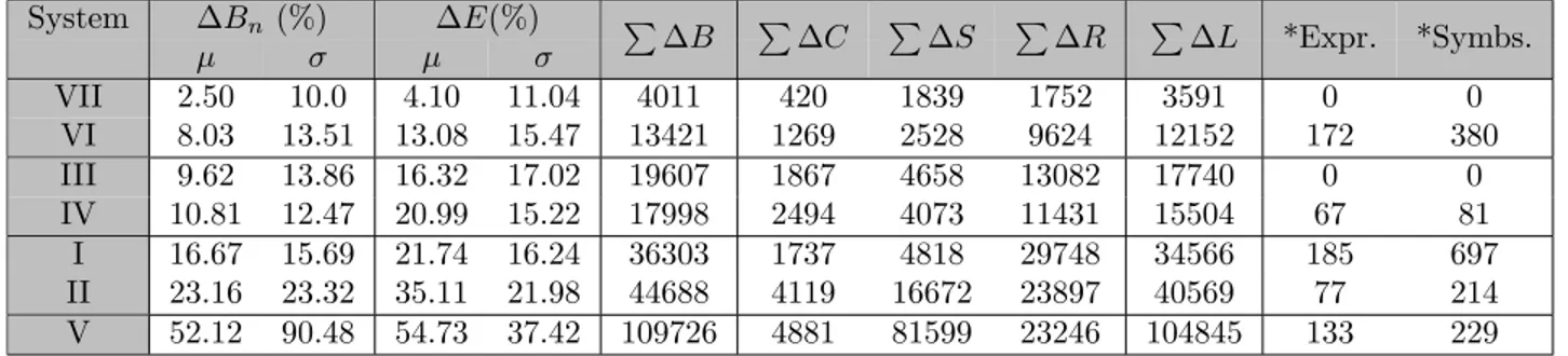
In Table 3, we present results for the CROHME 2012 systems again, but this time for metrics over label graphs created from the generated InkML output files. The metrics in Table 2 consider complete expressions (expression rate), objects (symbols: SYM Seg, SYM Rec), and abstract symbol layout from the MathML (STRUCT), along with the number of MathML abstract layouts that match ground truth after 1, 2 or 3 symbol or layout tag relabelings (REL-1/2/3). ST Rec, the percentage of strokes correctly labeled is directly related to ∆C, the number of mislabeled strokes. All other metrics in Table 3 are at the primitive level. In Table 3 systems are ranked by average label error per expression (∆Bn).
In Table 2, STRUCT and the symbol/stroke metrics are independent. It is possible for one of these to be 100%, and the other 0% within a single expression. In Table 3, ∆L is the number of segmentation and layout relationships between primitives that are correct. ∆S is the portion of ∆L specifically for segmentation edge errors (i.e. where at least one edge is labeled ’*’). The remaining incorrect edges (∆R) would quantify remaining incorrect relationships between primitives, and not the number of valid layouts as with STRUCT. ∆C is independent of ∆L, but deals only with symbol labels assigned to strokes.
Our evaluation tools were tested by reproducing the stroke recognition (ST Rec), symbol recall (SYM Seg), classification rate for correct symbols (SYM Rec) and expression rate (EXP) values shown in Table 2. In the process of doing this, we located some malformed output files, such as when symbols re-use a stroke. Shown in Table 3 are the number of expressions whose MathML symbol layout representation had structural errors, along with the number of concerned symbols: the most common problem is that some symbols are represented by tags (e.g. fraction lines, square roots), and some participants forgot to include the attribute associating tags with their corresponding symbol, or symbols were not referenced in the Presentation MathML output, leading them to be omitted in the label graph representation.
It is interesting that System IV has the third-best total sum of Hamming distances over all label graphs, ∆B (Table 3), but only the fifth-best expression rate (Table 2). Looking more closely, ∆E differs very little between systems IV and I, but the average ∆Bn differs by almost 6%, and the ∆B for system I is more than twice that for system IV. However, system I has nearly twice the layout recognition rate (STRUCT) and more than twice the expression recognition rate of system IV (Table2). A significant factor here, however, is that many System I outputs are malformed (185 expressions, containing 697 symbols).
System IV also had a lower ∆B than system III, which has an even higher expression rate. The symbol segmentation rate (Table 2) is nearly identical between Systems III and IV, but ∆S is slightly larger for System III. The number of correct layout relationships ignoring symbols and primitives is much higher (STRUCT), but ∆L is again larger for system III. However, System IV mislabels more strokes than System III, which significantly reduces the number of correct expressions (EXP), and ∆E due to the weighting of different error types. We can see that the average number of mislabelings for ∆Bn and ∆E reflect this increased per-expression label error, although total error is smaller. System III has more variance in accuracy at the primitive level, but higher accuracy at the level of individual expressions than System IV. The higher standard deviations for ∆Bn and ∆E in System III reflect this.
Systems II and V also change positions in Table 3 relative to Table 2. We can see in Table 2 that System II has a much higher symbol segmentation rate, which is consistent with the much smaller ∆S relative to System V. This leads to the change in their ranking in Table 3. However, although System V file produces many more malformed MathML expressions, more of the expressions that it processes are correct.
Table 3: CROHME part III Error Metrics for Label Graph Representations. Participant systems are ranked by average percentage error in label graphs (∆Bn). Shown are sums over all expressions for each Hamming distance (∆B, ∆C, ∆L and ∆S), along with distributions for ∆Bn and ∆E distributions shown by means (µ) and standard deviations (σ). The number of expressions (MathML) with formatting errors (*Expr.) and the number of concerned symbols (*Symbs.) in system outputs are provided. Systems IV and I and II and V switch positions relative to Table2
System ∆Bn (%) ∆E(%) µ σ µ σ P ∆B P ∆C P ∆S P ∆R P ∆L *Expr. *Symbs. VII 2.50 10.0 4.10 11.04 4011 420 1839 1752 3591 0 0 VI 8.03 13.51 13.08 15.47 13421 1269 2528 9624 12152 172 380 III 9.62 13.86 16.32 17.02 19607 1867 4658 13082 17740 0 0 IV 10.81 12.47 20.99 15.22 17998 2494 4073 11431 15504 67 81 I 16.67 15.69 21.74 16.24 36303 1737 4818 29748 34566 185 697 II 23.16 23.32 35.11 21.98 44688 4119 16672 23897 40569 77 214 V 52.12 90.48 54.73 37.42 109726 4881 81599 23246 104845 133 229
Some additional useful information can be found in the confusion matrix for stroke and stroke relationship classification. For example, for System VII, the most frequent confusion in ∆L is between no relationship (’ ’) and the adjacent-at-right (’R’) relation. This reflects that many symbols end up on incorrect baselines, and because of the inheritance of spatial relations from parents, this generates many lost adjacencies present in the ground truth layout tree.
This first case study illustrates that we can obtain a primitive-level analysis that usefully complements information from object level metrics such as symbol recognition rates, and recall and precision. We do not show this here for space, but the label graph representation also permits common and distinct errors between label graphs to be computed in a straightforward manner. We believe that this will be useful for constructing parser ensembles and use in machine learning algorithms operating at the level of complete graphs (e.g. using neural networks, or AdaBoost).
5. UNDIRECTED GRAPHS AND MULTIPLE LEVELS OF STRUCTURE
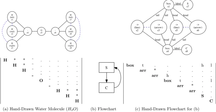
Modifying label graphs to represent undirected graphs is straightforward. Consider an undirected graph repre-senting connections between symbols in a handwritten diagram for a water molecule, such as shown in Figure 4. Here each (H)ydrogen symbol is written using three strokes: the left vertical stroke, following by the horizontal stroke, followed by the right horizontal stroke. In the label graph, connection of a primitive to a bond is indicated by a tilde (‘˜’), with segmentation (’*’) and no relationship labels as a dot (‘.’). The graph captures the set of element symbols and bonds, and which elements connect to each bond. Figure 4 provides another example of an undirected graph representation for a simple directed flowchart with a cycle that represents a segment-classify cycle.
We can use directed label graphs to represent the directed graph equivalent of an undirected graph. But the undirected label graph is more intuitive, and reduces the number of comparisons for the Hamming distance (∆B) by about half, from n2 to (n2+ n)/2 comparisons. Our directed graphs can also be treated this way, by requiring that both directed labels match for a pair of primitives in order to be correct.
More complex structures may also be represented using a related set of label graphs with common primi-tives, such as when an expression contains matrices. In this case, at one level objects are matrix cells defined over primitives and their relationships, and at another level objects are primitives grouped into symbols, with structures similar to our earlier examples. As a more complex example, one might define multiple label graphs in ground truth for text, figures, tables, images, where each is defined over the set of connected components in a document image. A drawback for evaluation is the large number of primitives involved, making metrics expensive (using sets to represent labels across levels of structure may mitigate this cost). Evaluating at the level
H (left) s1 H (mid) s2 H (right) s3 -s4 s5O s6 -H (left) s7 H (mid) s8 H (right) s9 H * * ˜ . . . . . H * ˜ . . . . . H ˜ . . . . . - ˜ . . . . O ˜ . . . - ˜ ˜ ˜ H * * H * H (a) Hand-Drawn Water Molecule (H2O)
S C (b) Flowchart box s1 S s7 label -> (line) s2 tail -> (arrow) s3 tail box s4 label s8C -> (line) s5 tail -> (arrow) s6 tail head head head head box t . . . . h l arr * . . . . . arr h . . . . box t . . l arr * . . arr . . S . C (c) Hand-Drawn Flowchart for (b)
Figure 4: Undirected Structure for a Hand-Drawn Chemical Diagram and Flowchart. (b) represents an iterative process with a flowchart diagram. (c) identifies which ends of detected arrows connect to a box in (b) using “tail” or “head”, and which primitives “label” boxes
of pixels in images is theoretically possible, but may be impractical. Consider computing ∆B for a 1000x1000 image, requiring one trillion comparisons for a single label graph in the worst case.
6. CONCLUSION
We have introduced primitive label graphs as a means for representing and evaluating recognized structure, using the recognition of handwritten mathematics for illustration. This representation may be used to capture obtain new primitive-level metrics based on Hamming distances that characterize classification, segmentation, parsing and overall structural differences between two structural interpretations of a given set of input primitives. Using the CROHME 2012 data we have illustrated how these metrics complement conventional metrics such as recognition rates, recall and precision by offering a lower level of granularity for analysis. Label graphs have already been used for information retrieval (retrieving individual LaTeX expressions), and might be used in machine learning algorithms to produce parser combinations, and induce parsers from label graph data.
ACKNOWLEDGMENTS
Our thanks to Bertrand Co¨uasnon and Aur´elie Lemaitre and the anonymous reviewers for helpful feedback, and to the CROHME 2012 participants for sharing their system outputs. We also thank the Universit´e de Nantes (IUT) for providing the first author with a Visiting Professorship in support of this research. This material is based upon work supported by the National Science Foundation (USA) under Grant No. IIS-1016815.
REFERENCES
[1] Lapointe, A. and Blostein, D., “Issues in performance evaluation: A case study of math recognition.,” in [Proc. Int. Conference on Document Analysis and Recognition ], 1355–1359 (2009).
[2] Awal, A.-M., Mouch`ere, H., and Viard-Gaudin, C., “The problem of handwritten mathematical expression recognition evaluation.,” in [Proc. of International Conf. Frontiers in Handwriting Recognition ], 646–651 (2010).
[3] Rice, S. V., Kanai, J., and Nartker, T. A., “An algorithm for matching ocr-generated text strings.,” Inter-national Journal of Pattern Recognition and Artificial Intelligence 8(5), 1259–1268 (1994).
[4] Mouch`ere, H., Viard-Gaudin, C., Kim, D. H., Kim, J. H., and Utpal, G., “ICFHR 2012 - competition on recognition of on-line mathematical expressions (CROHME 2012),” in [Proc. of Int. Conf. on Frontier in Handwriting Recognition ], (2012).
[5] Schellenberg, T., Layout-Based Substitution Tree Indexing and Retrieval for Mathematical Expressions, mas-ter’s thesis, Rochester Institute of Technology, Rochester, NY, USA (2011).
[6] Mouch`ere, H., Viard-Gaudin, C., Kim, D. H., Kim, J. H., and Utpal, G., “CROHME2011: Competition on recognition of online handwritten mathematical expressions,” in [Proc. Int. Conference on Document Analysis and Recognition ], 1497–1500 (2011).
[7] Zanibbi, R., Blostein, D., and Cordy, J., “A survey of table recognition: Models, observations, transforma-tions, and inferences,” International Journal of Document Analysis and Recognition 7, 1–16 (2003). [8] Zanibbi, R., Pillay, A., Mouch`ere, H., Viard-gaudin, C., and Blostein, D., “Stroke-based performance
met-rics for handwritten mathematical expressions,” in [Proc. of Int. Conference on Document Analysis and Recognition ], 334–338 (2011).
[9] Zanibbi, R. and Blostein, D., “Recognition and retrieval of mathematical expressions,” International Journal of Document Analysis and Recognition 15(4), 331–357 (2012).
[10] Liang, J., Document Structure Analysis and Performance Evaluation, phd thesis, University of Washington, USA (1999).
[11] Phillips, I. T. and Chhabra, A. K., “Empirical performance evaluation of graphics recognition systems.,” IEEE Transaction Pattern Analysis and Machine Intelligence 21(9), 849–870 (1999).
[12] e Silva, A. C., “Metrics for evaluating performance in document analysis: application to tables.,” Interna-tional Journal of Pattern Recognition and Artificial Intelligence 14(1), 101–109 (2011).
[13] Garain, U. and Chaudhuri, B. B., “Recognition of online handwritten mathematical expressions.,” IEEE Transactions on Systems, Man, and Cybernetics, Part B 34(6), 2366–2376 (2004).
[14] Chan, K.-F. and Yeung, D.-Y., “Error detection, error correction and performance evaluation in on-line mathematical expression recognition.,” Pattern Recognition 34(8), 1671–1684 (2001).
[15] Sain, K., Dasgupta, A., and Garain, U., “Emers: a tree matching-based performance evaluation of mathe-matical expression recognition systems,” International Journal of Document Analysis and Recognition 14(1), 75–85 (2011).
[16] Hu, J., Kashi, R. S., Lopresti, D. P., and Wilfong, G. T., “Evaluating the performance of table processing algorithms.,” International Journal of Document Analysis and Recognition 4(3), 140–153 (2002).