Underwriting Apophenia and Cryptids: Are Cycles Statistical Figments of our Imagination?

Texte intégral

(1)2013s-07. Underwriting Apophenia and Cryptids: Are Cycles Statistical Figments of our Imagination? M. Martin Boyer. Série Scientifique Scientific Series. Montréal Mars 2013. © 2013 M. Martin Boyer. Tous droits réservés. All rights reserved. Reproduction partielle permise avec citation du document source, incluant la notice ©. Short sections may be quoted without explicit permission, if full credit, including © notice, is given to the source..

(2) CIRANO Le CIRANO est un organisme sans but lucratif constitué en vertu de la Loi des compagnies du Québec. Le financement de son infrastructure et de ses activités de recherche provient des cotisations de ses organisations-membres, d’une subvention d’infrastructure du Ministère du Développement économique et régional et de la Recherche, de même que des subventions et mandats obtenus par ses équipes de recherche. CIRANO is a private non-profit organization incorporated under the Québec Companies Act. Its infrastructure and research activities are funded through fees paid by member organizations, an infrastructure grant from the Ministère du Développement économique et régional et de la Recherche, and grants and research mandates obtained by its research teams. Les partenaires du CIRANO Partenaire majeur Ministère de l'Enseignement supérieur, de la Recherche, de la Science et de la Technologie Partenaires corporatifs Autorité des marchés financiers Banque de développement du Canada Banque du Canada Banque Laurentienne du Canada Banque Nationale du Canada Banque Scotia Bell Canada BMO Groupe financier Caisse de dépôt et placement du Québec Fédération des caisses Desjardins du Québec Financière Sun Life, Québec Gaz Métro Hydro-Québec Industrie Canada Investissements PSP Ministère des Finances du Québec Power Corporation du Canada Rio Tinto Alcan State Street Global Advisors Transat A.T. Ville de Montréal Partenaires universitaires École Polytechnique de Montréal HEC Montréal McGill University Université Concordia Université de Montréal Université de Sherbrooke Université du Québec Université du Québec à Montréal Université Laval Le CIRANO collabore avec de nombreux centres et chaires de recherche universitaires dont on peut consulter la liste sur son site web. Les cahiers de la série scientifique (CS) visent à rendre accessibles des résultats de recherche effectuée au CIRANO afin de susciter échanges et commentaires. Ces cahiers sont écrits dans le style des publications scientifiques. Les idées et les opinions émises sont sous l’unique responsabilité des auteurs et ne représentent pas nécessairement les positions du CIRANO ou de ses partenaires. This paper presents research carried out at CIRANO and aims at encouraging discussion and comment. The observations and viewpoints expressed are the sole responsibility of the authors. They do not necessarily represent positions of CIRANO or its partners.. ISSN 1198-8177. Partenaire financier.

(3) Underwriting Apophenia and Cryptids: Are Cycles Statistical Figments of our Imagination? * M. Martin Boyer†. Résumé/Abstract The Lloyd’s 2007 Survey of Underwriters states that "for the third year running, managing the cycle emerged as the most important challenge for the industry, by some margin". The contention is of course that underwriting cycles exist in property and casualty insurance and are economically significant. Using a meta-analysis of published papers in the area of insurance economics, I show that the evidence in favor of underwriting cycles is misleading or even completely absent. There is in fact no statisical or economic support for the existence of underwriting cycles. This means that firm profitability in the property and casualty insurance industry is not cyclical; we only observe profitability going up or down with no meaningful pattern. It consequently follows that pricing in the property and casualty insurance industry is not incompatible with that of a competitive market. Mots clés/Keywords : Property and liability insurance, underwriting profits, insurance pricing. Codes JEL : G22.. *. This research was financially supported by the Social Science and Humanities Research Council of Canada. I am indebted to J.-François Outreville, Simon van Norden, Éric Jacquier and Michael Powers for comments on an earlier draft, as well as to Tolga Cenesizoglu for continuing discussions. I would also like to thank conference participants at the Munich Behavioral Insurance Seminar for listening to a previous iteration of this research project, and to 2012 EGRIE participants in Palma – and especially Richard Peter - for very stimulating discussions. † CEFA Professor of Finance and Insurance and Cirano Fellow, Department of Finance, HEC Montréal (Université de Montréal). 3000, chemin de la Côte-Sainte-Catherine, Montréal QC, H3T 2A7 Canada; martin.boyer@hec.ca..

(4) Underwriting Apophenia and Cryptids: Are Cycles Statistical Figments of our Imagination? 1. Introduction. Ever since Brocket and Witt (1982) showed that insurer profitability is well explained by an AR(2) process, insurance academics, as well as practitioners,1 have presumed that profitability cycles exist2 in the property and casualty insurance industry, but not in the life insurance industry. Winter (1991) states that "the existence of cycles in insurance markets is a central topic of insurance literature" (p.117). One can read in Lloyd’s 2007 Survey of Underwriters that "for the third year running, underwriters in the Lloyd’s market have identified managing the cycle as the most important challenge for the industry". These underwriting cycles appear to happen at regular intervals in many OECD countries if one was to look at the plethora of available evidence (see Venezian, 1985, Cummins and Outreville, 1987, Lamm-Tennant and Weiss, 1997, Chen et al., 1997, and Meier, 2006b, inter alia). These cycles are characterized by periods of high profitability followed by periods of low profitability. The existence of a predictable underwriting cycle has been seen as a sufficient condition for concluding that insurance markets are inefficient (see Gron, 2010, or Outreville, 1990), so that government intervention could be warranted (see Winter, 1991, for the argument that government intervention would exacerbate cycles). Another reason why cycles can become the catalyst for government intervention is that underwriting cycles have been associated in Trufin et al. (2009) with higher ruin probability. The thesis I defend in this paper is that the statistical evidence in favor of the existence of cycles is week, and economically and statistically insignificant (see also Venezian, 2006). The reason is that the tests that have been used in previous research on underwriting cycles were biased in favor of finding such cycles, so that any inference and/or conclusion drawn from these tests are necessarily misleading. Once these biases 1 In Lloyd’s Annual Report 2006, one can read that "there is an increasingly complex underwriting cycle, where loss trends and market forces are driving cycles with characteristics that differ by line of business and territory". In a McKinsey 2008 report, one can read that "reliance on the cycle and expectations of its implications for underwriting and profits are common across the P&C insurance industry."See also Clark (2010), as cited in Wang et al. (2010) 2 In the first sentence of Doherty and Garven (1995, p.383) we can read that "It is widely believed that insurance markets are cyclical"; Derien (2008, p.1) writes that "the presence of the underwriting cycle in non-life insurance is well established"; Wang et al. (2010, p.7) write that "the existence of the underwriting cycle is undeniable"; Lamm-Tennant et al. (1992, p.426) talk about "the well-known cyclical pattern in loss ratios over time"; Chen et al. (1999, p.30) mention that the "existence of an underwriting cycle has been recognized by researchers"; Harrington and Niehaus (2001, p.658) assert that "conventional wisdom among many practitioners and other observers is that soft and hard markets occur in a regular cycle, commonly known as the underwriting cycle"; Meier (2006a, p.65) contends that "there seems to be a wide consent in the insurance cycles literature ... that the American insurance industry can be characterized by cycles of about six years in length"; a 2002 European Commission study affirms that "in the non-life insurance market one of the major market drivers is the insurance cycle"; Fitzpatrick (2004, p.257) writes that "there are, in fact, as many underwriting cycles as there are products in the property and casualty insurance market", which is a rephrasing of Stewart’s (1984, p.305) "not every line of insurance experiences the same phase at the same time". One can even read on Wikipedia (http://en.wikipedia.org/wiki/Insurance_cycle, consulted last on 13 July 2012) that "the insurance cycle is a phenomenon that been recognised since at least the 1920s. Since then it has been considered an insurance fact of life".. 2.

(5) have been corrected, significant underwriting cycles become the exception rather than the norm. As I will show in this paper, we cannot scientifically dismiss the absence of cycles (i.e., we cannot reject H0), so that scientific rigor demands that we cannot dismiss that insurer profitability is unpredictable and that it follows a random walk. Consequently, Lloyd’s contention that we can "manage the cycle"3 is a waste of resources. Although many sound theories have been developed to explain the existence of underwriting cycles in the property and casualty insurance industry,4 I will conclude in this paper that insurance economists have suffered from apophenia (that is, they have reported seeing meaningful patterns in random or meaningless data).5 In that sense, insurance economists have been looking for a underwriting cryptid;6 that is, a phenomenon that exists only in our collective (and overacting) imagination (see also Powers, 2012, who uses the term "pareidolia"7 instead of "apophenia"). Sterman (1994) and McFadden (1999) call this search for confirmation of current beliefs a quest for “emotional and spiritual sustenance”. Another bias, which is called selective memory, occurs when favorable or unfavorable events that fit with an agent’s prior are remembered more readily than events that do not fit.8 McFadden (1999) adds: "Both selective memory and selective search cause individuals to be superstitious, perceiving correlation between their own actions and outcomes of random events even when such correlation is implausible. Superstition appears irrational, but may in fact be consistent with a complex nonergodic world view in which a Bayesian never accumulates sufficient objective data to rule out a mental model in which Nature is conspiratorial and personal" (p.93). My conclusion will not be that insurance prices and insurer profitability are not affected by external or internal shocks; rather, it will be that there is no evidence that such shocks are anything else than random unpredictable occurences. As I will show, any Brownian motion time series has a (high) probability of resulting in a cycle as defined in the underwriting cycle litterature. The current paper offers a complement to Boyer et al. (2012) who show that there is no in-sample or out-of-sample evidence that would support the view that there is any type of predictability in annual insurance underwriting performance in the United States. Put differently, no evidence exists that would allow one to conclude against the null hypothesis of speculative efficiency. The results in the current paper suggest not only that cycles are on the whole 3 http://www.lloyds.com/Lloyds/Press-Centre/Press-Releases/2006/12/Seven_steps_to_managing_the_cycle 4 A non-exhaustive list includes the following contributions: Forecasting errors (Venezian, 1985, Boyer at al., 2011), delayed feedback of prices to profits (Berger, 1988), insurer moral hazard (Harrington and Danzon, 1994. Fitzpatrick, 2004), arbitrage theory (Cummins and Outreville, 1987), risky debt (Cummins and Danzon, 1997), interest rate variations (Fields and Venezian, 1989), and capacity constraints (Gron, 1994, Niehaus and Terry, 1993, and Winter, 1994). 5 See http://etyman.wordpress.com/2010/01/29/apophenia/ or http://en.wikipedia.org/wiki/Apophenia. 6 Zombies, werewolves and leprechauns are famous cryptids. Other cryptids include: Bigfoot, Mapinguari, Sasquatch, Yowie, Yeti, bunyip, chupacabra, fairies, the Loch Ness monster, mokele mbembe, mothman, unicorns, vampires, and p-zombies. See The Skeptic Dictionnary (http://skepdic.com/ticrypto.html, last visited on 10 September 2012) or Carroll (2003). 7 Defined in Powers (2012) as a phenomenon "in which a person belives that he or she sees systematic patterns in disordered and possibly entirely random data" (p. 192). 8 To paraphrase recent Bud light commercials: "it’s only stupid if it doesn’t work".. 3.

(6) unpredictable so that sophisticated underwriters should be unable to forecast future changes in industry profitability, but also, and perhaps more importantly, that cycles may not even exist. This short paper is organized as follows. Section 2 summarizes the classic property and casualty insurance underwriting cycles papers that I will use in my meta-analysis. Section 3 presents the methodology I use to analyse the likelihood that cycles will occur in any time series. The paper’s main results (i.e., the different statistical tests) are also presented in Section 3. I conclude in Section 4.. 2. Insurance cycles. Many theories have been proposed to explain the existence of underwriting cycles as defined in Brocket and Witt (1982). Although it is not my goal to present all of them − the interested reader is invited to read the excellent surveys of Harrington (2004), Meier and Outreville (2006) and Wang et al. (2010) − some are more important as they either were the seed from which the entire cycle literature grew, or have kept the topic alive. Cummins and Outreville (1987) propose that cycles were the result of external factors, such as institutional and regulatory lags, as well as accounting practices. They contend that even though premiums and profit margins are rationally set to reflect all available information, cycles could arise because of external factors that vary across countries because of their different regulations and regulatory lags. In the same vein, Venezian (1985) suggests that fluctuations in underwriting profit margins are caused by adaptive rate-making methods. He states that the methods used by insurers to forecast future rates induce cycles. Consequently, insurer profitability should be the combination of a predicable cyclical component and of random components (see also Lamm-Tennant et al., 1992, Harrington and Yu, 2003, and Boyer et al., 2012). Harrington and Danzon (1994) propose that cycles are partly caused by insurers that are betting for ressucitation; an insurer with depleted assets − because of large losses, say − is tempted to sell its products at too low a price in an attempt to improve its market share. This mispricing of insurance can also stem from heterogeneous information (see also Fitzpatrick, 2004). Both cases induce insurers to cut their prices to protect their market share. Harrington and Danzon (1994) find support for their hypothesis as forecast revisions and prices are inversely related.9 Another asymmetric information approach is that of Cummins and Danzon (1997) whereby the price of insurance is inversely related to the insurer’s default risk. As insurers raise capital in response to adverse shocks, their loss ratio should be inversely related to their default risk, which means that insurance premiums should be positively correlated to financial quality.10 Niehaus and Terry (1993) observe cases of premiums being determined by past losses, and even stronger evidence that they are determined by the industry’s past surplus. Their findings support the hypothesis that underwriting cycles are partly the result of costly external capital. Citing Winter (1994), Cummins and Danzon (1997) 9 See 1 0 See. also Harrington (2004), Baker (2005) and Alkemper and Mango (2005). also Doherty and Kang (1988) and Doherty and Garven (1992).. 4.

(7) and Cummins and Doherty (2002), Cummins (2006) writes that the "consensus in the economics literature is that hard and soft markets are driven by capital market and insurance market imperfections such that capital does not flow freely into and out of the industry in response to unusual loss events" (p. 345). Similar to Brocket and Witt (1982), Harrington and Niehaus (2000) find that insurance prices follow a second order autoregressive process, and then focus on capital shock models to explain both hard and soft market periods in the insurance industry. They suggest that premium variations are partly due to variations in fundamentals. They also argue that there is evidence of another form of variation that cannot be explained by efficient market theories. They attribute these variations to capital shocks. This follows the capacity-constraint theory argument that underwriting cycles are the result of frictions caused by a temporary incapacity of the industry to insure all risks (see in particular Gron, 1994a, 1994b, and Winter, 1994), or the impact of a major catastrophe (see Cummins, 2006, and Born and Viscusi, 2006) that depletes part of the capital in the reinsurance market (see Berger et al., 1992, and Meier and Outreville, 2006).11 As insured risks are not independent, premium nonlinearity are the result of the dependence between losses. Because of this dependence conditional on the events occurring, and because raising external capital is more costly than internal capital, market capacity is determined by the insurers’ net worth since it is necessary to cover the contractual promise to pay claims. None of these theories (and others I might have forgotten) about why underwriting cycles exist have wondered if they actually exist.12 The presumption has been that underwriting cycles as define in Brocket and Witt (1982) exist, and have existed since the early 1920s . The purpose of this paper is to question the economic and statistical existence of underwriting cycles using the same evidence that has been presented to support their apparent existence.. 3. Source for the meta-analysis. The insurance industry goes through periods of high and low premiums relative to losses. The succession of peaks and troughs has produced a large literature13 that attempts to explain why insurance markets cycle through such periods of high and low profitability. The typical approach14 used to examine cycles in the property and casualty insurance industry is based on standard econometric models (see Stock and Watson, 1988, Nelson and Plosser, 1982) that can be represented as: Φ() =  + .  ∼ N(0 ). 1 1 More. (1). naive capacity constraint models were developped earlier by Stewart (1981,1984) and Wilson (1981). only exception I found is Cummins and Outreville (1987, p.249) who write that "if cycles exist in insurance markets". 1 3 The academic and professional literature generally agrees that there has been seven underwriting cycles in the United States since 1950. 1 4 An alternate approach is to use spectral analysis as in Venezian (2006) and Venezian and Leng (2006). But as highlighted in Venezian (2006), spectral analysis is dominated by a standard AR(2) approach for the purpose of analyzing underwriting cycles. See Chapter 6 in Hamilton (1994) for more on spectral analysis. 1 2 The. 5.

(8) where  is the profitability measure (underwriting ratio, loss ratio, combined ratio, or any other measure of insurer profitability), and Φ() is a polynomial of degree  in the backshift operator  (see Boyer et al., 2012, for more details) When   1, the characteristic equation may have pairs of complex roots, if the corresponding determinant is negative. Then, for each such pair, of norm |||| and real part R(), there is a cycle in the autocorrelation of  , with period: =. 2 2 ³ µ ´= R() arccos |||| arccos √1 2. −2. ¶. (2). This suggests a maximum likelihood estimator of  based upon the maximum likelihood estimator of the complex roots, which itself follows from the maximum likelihood estimators of Φ, the vector of autoregressive parameters in equation 1. In particular, when we examine autoregressive models of the second order (i.e., AR(2) models), we will have two autoregressive parameters in equation 1. Let us call 1 the one-period lag coefficient and 2 the two-period lag coefficient. Assuming that we only take the positive root of. p −2 and that 1 ≥ 0, we know that  is bounded. below at 4. In other words, it is impossible to obtain a cycle that would be less than 4 since arccos (0) = 2, so that  1 =0 = 4.. 3.1. Data collection. I collected the AR(2) coefficients from a set of papers that examine the existence of cycles in different countries, in different periods, and in different property and casualty lines of business: Venezian (1985), Cummins and Outreville (1987), Chen et al. (1997), Harrington and Niehaus (2000), Meier (2006a, 2006b) and Meier and Outreville (2006). I also used my own calculations using data provided by A.M. Best’s Aggregates & Averages for the United States (see also Wang et al., 2010) and by the Insurance Bureau of Canada for Canada, as used in Trufin et al. (2009). As can be seen from Table 1 in the Appendix, this exercise yields a total of 98 regressions that cover different periods, different countries and different econometric specifications. There is also another set of 96 time series of insurer profitability that were studied by Lamm-Tennant and Weiss (1997), for which none of the AR(2) coefficients are provided and that will not be included in the final analysis . Table 2 presents the summary statistics associated with the different15 samples and sub-samples examined. It is important to note that there is no statistical difference (two-tail test at the 5% level) between the average cycle lengths between the Lamm-Tennant and Weiss (LTW) sample (59 data points) and the sample I am using (the 69 data points under column SE available ALL), especially if we remove the longest cycle (28 years) that was obtained after performing a regression without a trend component using U.S. data from 1 5 The. criterion used for the different subsamples is described later in the paper.. 6.

(9) 1969-2004.16 A non-parametric Kolmogorov-Smirnov test on the two samples tells us, however, that the two distributions of cycle lengths are not equal and not normally or log-normally distributed, thus biasing the student equality test used on the means of the two samples. I will not include in my final analysis the 96 regression results of Lamm-Tennant and Weiss (1997) because the authors did not report the standard errors or the t-statistics of their AR(2) estimates.17 Table 2. Summary statistics of cycles in the different SE available Combo ALL Signif. Bonf. Total Observations 194 98 98 98 Number of cycles 128 69 30 21 Probability of a cycle 66% 70% 31% 22% Mean cycle length (or period) 7.62 8.11 7.03 6.89 Median cycle length 6.90 7.70 6.95 6.51 St.Dev. of cycle length 3.37 3.51 1.31 1.32 Skewness of cycle length 3.08 3.33 0.43 0.89 Kurtosis of cycle length 13.83 16.44 -0.66 0.28 Longest cycle 28.40 28.40 9.92 9.92 Shortest cycle 4.09 4.36 5.17 5.24 Gaussian (JB-test)18 Reject Reject Don’t Don’t Gaussian (KS-test)19 Reject Reject Don’t Don’t Gaussian (SW-test)20 Don’t Don’t. samples and subsamples Stud. 98 11 11% 6.08 6.11 0.57 0.94 1.24 7.35 5.39 Don’t Don’t Don’t. LTW 96 59 61% 7.05 6.15 3.12 2.89 10.54 21.97 4.09 Reject Reject. Random 700*200 66% (3%) 8.6 (12) 6.0 (03) 9.8 (9) 5 (22) 35 (30) 10,000 4 Reject. Trunc. 140,000 91000 65% 7.50 5.95 4.25 2.3 6.1 30 4 Reject. LTW refers to the results from Lamm-Tennant and Weiss (1997). SE available refers to those studies where the standard errors of the two AR(2) regression coefficients are available. ALL uses all the data points; Signif uses all data points where the two coefficients are significantly different from zero; Bonf uses the data points where the two coefficients pass the Bonferroni test, and Stud uses the data points where the two coefficients pass the Student test. Combo combines the 98 observations where standard errors are available with the 96 observations presented in Lamm-Tennant and Weiss (1997). Random and Trunc refer to the case where 1 and 2 were each randomly drawn from a uniform distribution. The values under the Random column are the average values for each statistical moment using 700 series of 200 draws with the standard deviation in parentheses. The values under the Trunc column were obtain using 140,000 draws, but limiting the maximum cycle length to 30 years. 1 6 I also analyzed the 1874-1901 U.S. fire insurance experience reported in Baranoff (2003), the 1874-1906 fire insurance industry loss ratio reported in Zanjani (2004), the recent data from 1992 until 2011 reported in Hartwig (2011) for P&C commercial lines, homeowner and workers’ compensation, and South African marine insurance data from Tarr (2008). Because these are not traditionnal papers cited in the literature, I will not use them in the overall analysis, but their inclusion would not change the conclusion of the paper. For the record, the data in Baranoff (2003) and Zanjani (2004) do not yield cycles as defined in Brocket and Witt (1982) since both 1 and 2 parameters are positive, and only one of the three time series data in Hartwig (2011) yields such a cycle. Finally, I found only one cycle out of the the two time series of Tarr (2008). 1 7 I contacted Mary Weiss who could not find the raw data they used for that paper. 1 8 The Jarque-Bera test (see Jarque and Bera, 1980) examines whether the observation are distributed normally based on the  . observed skewness and kurtosis. The JB statistic is given by  =.  6. 2 +. (−3)2 4. , with  being the number of observations. and  and  being the third and fourth moment of the empirical distribution (not the kurtosis which is the fourth central 3(−1)2. moment from which we substract (−2)(−3) ). The JB statistic follows a 2 distribution with two degrees of freedom. 1 9 The Kolmogorov-Smirnov test of normality is valid only for a number of observations between 10 and 1024. We present the 5% test here so that we cannot reject the normality distribution assumption with a 95% confidence interval. http://www.physics.csbsju.edu/stats/KS-test.n.plot_form.html 2 0 The Shapiro-Wilk test of normality is valid only for a small number of observations (between 5 and 38). We present the 5% test here so that we cannot reject the normality distribution assumption with a 95% confidence interval. See Shapiro and. 7.

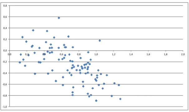
(10) Using the Jarque-Bera statistical test or running the non-parametric Kolmogorov-Smirnov normality test, I am able to reject that the period of cycles is distributed normally for the three largest samples (under the column headings Combo, ALL, LTW ). For the three smaller samples (Signif, Bonf and Stud ), the JarqueBera test, the Kolmogorov-Smirnov test, and even the small sample Shapiro-Wilk test tell us that we cannot reject the normality distribution assumption at the 95% level of confidence. Figure 1 presents the point estimates of the 98 1 and 2 regression results for which I have the standard error of the AR(2) regression and that are displayed in Table 1 in the Appendix.21 0,8. 0,6. 0,4. 0,2. 0,0 0,0. 0,2. 0,4. 0,6. 0,8. 1,0. 1,2. 1,4. 1,6. 1,8. 2,0. ‐0,2. ‐0,4. ‐0,6. ‐0,8. ‐1,0. Figure 1: AR(2) regression coefficients for each time series; one-lag parameter value (1 ) on the horizontal axis and two-lag parameter value (2 ) on the vertical axis. The last two columns of Table 2 present the average statistics associated with cycle lengths when I draw randomly 1 and 2 from uniform distributions over the acceptable domains of each parameter (i.e., 1 ∈ [0 2] and 2 ∈ [−1 0]). The Random column displays the average cycle length statistics (and standard deviation) when 700 series of 200 random draws of 1 and 2 are used. Using the same 140,000 random draws of 1 and 2 , the last column (Trunc) concentrates on the basic statistics obtained when I limit the longest cycle to be 30 years (the maximum cycle length that is observed in the first six columns). It is interesting to note the similarities between the basic statistics (mean, median, standard deviation, skewness and kurtosis) of the cycle lengths of the first column (Combo) and the last two columns (Random and Trunc). Wilk (1965) for more details. 2 1 Figure A in the appendix highlights the source of some of those points by seperating results that are problematic for the theory of cycles in P&C insurance, from results that are less problematic. Many of the classical results are clustered.. 8.

(11) For instance, the mean of the cycle period under the column Combo is not statistically different from the cycle period mean under the column Trunc.. 3.2. Statistical tests and methodology. The hypothesis I test with the set of results that was published in the academic literature is the following: • H0: Insurance profitability cycles do not exist • H1: Insurance profitability cycles exist Of the 98 regression results under column All of Table 1, only 69 are such that we can actually calculate a cycle period. Figure 2 illustrates how many of the 98 regression results displayed above yield a cycle. The square data points represents regression results for which a cycle cannot be computed. The observations represented by diamond-shaped points22 are such that the 1 and 2 values allow the calculation of an underwriting cycle period.. Figure 2: AR(2) regression coefficients for each time series; one-lag parameter value (1 ) on the horizontal axis and two-lag parameter value (2 ) on the vertical axis. Cycle period cannot be computed for the observations reported as squares. If I am to add the 59 instances of cycles presented in Lamm-Tennant and Weiss (1997) out of the 96 regressions they conducted (12 countries, 8 lines of business), the proportion of instances where a cycle is presumably observed is 128/194=66%, as can be seen under the column Combo in Table 1. How significant is the 66% likelihood of observing a cycle? 2 2 Excluding the data points from Lamm-Tennant and Weiss (1997) for which the first and second lag coefficient values are not reported, the square data points represent 70% of the total number of observations.. 9.

(12) Suppose we have no knowledge whatsoever about the values of 1 and 2 other than imposing stationarity on the AR(2) process. Suppose also that we draw randomly from a uniform distribution values for 1 and 2 . Given a random uniform distribution of 1 and 2 , the probability of observing a cycle can easily be shown by analytical integration to be 66%. As shown in Figure 3, this probability of observing a cycle is equal to the area below the parabola 21 + 42  0 and above the base of the base of the triangle set at 2 = −1 where the AR(2) has two complex roots (see Zellner, 1971, and Sargent, 1986). I am now able to rewrite the hypothesis that I test in terms of the 1 and 2 parameters: • H0: 2 ≤ − • H1: 2  −. 21 4 21 4. and 1 ≥ 0 or 1  0. Figure 3: AR(2) regression coefficients for each time series; one-lag parameter value (1 ) on the horizontal axis and two-lag parameter value (2 ) on the vertical axis. Cycle period cannot be computed for the square data points because they lie above the parabola. The straight line represents the upper limit of the stationarity triangle. Drawing randomly 1 and 2 from a uniform distribution would give us a pair of parameter values such that a cycle "exists" with probability 66%. Even if I let 2 take potential positive values, but that all 1 and 2 couples remain within the stationarity triangle admissible in an AR(2) process (the dark straight line with slope −1 in Figure 3), the area under the parabola represents 2/3 of the entire area of the stationarity triangle. Consequently, the likelihood that one has found a cycle in any time series of insurance profitability is not very different from the probability that a spurious cycle is found in a pure random distribution of the two lagged parameters. 10.

(13) Also worth mentioning is that not all regression results presented in Table 1 have regression coefficients that are significant. In fact, of the 98 regression results under study, only 30 actually have the 1 and 2 coefficients that are both significantly different from 0.23 In other words, more than half of the regressions where a cycle has been presume to exist are subject to important errors in variable problems. Another interesting observation is that the real test one should conduct is not for the 1 and 2 coefficients to be different from zero, but to be different from the parabola that delimits the existence or not of a cycle. Surprisingly, no one in the literature has conducted a joint significance test on the two parameters of interest. Using a Bonferroni test or a Student test reduces even more the likelihood that a cycle is observed. The Bonferroni test is a simple conservative joint estimation test whereby if there are two parameters of interest in a regression, then the Bonferroni p-value of the joint test is equal to twice the highest p-value. For example, if the two coefficients have individually p-values of 1% and 3%, the combined p-value is 2×max [1% 3%] = 6%. q The Student test is computed as (1 + 42 )  (1 )2 + (42 )2 , where I assumed that the covariance between the 1 and 2 estimates is zero. It is important to note that neither test is precise: The Bonferroni test by. design, and the Student test by absence of data since I do not have any of the covariances between the two AR(2) estimates. Figure 4 highlights the correspondence of parameter values between observations that do not have the two parameters that are statistically different from zero (Insignificant), the 30 observations (Significant) whereby the two are statistically different from zero but do not pass the Bonferroni test, the 21 observations (Bonferroni) whereby the parameters pass the Bonferroni test but not the Student test, and finally the 11 observations (Student) that pass all tests, including the most stringent Student test.24 If I only focus on the observations that pass the Bonferroni test, there are merely 21 observations whereby it would be reasonable to believe that a cycle exists out of the 98 observations I started with. This represents a success ratio of 22%. These 21 observations allow me to calculate an average cycle period of 6.9 years (median of 6.5 years) and a standard deviation of 1.3 years. The average cycle period is smaller than the mean of the randomly obtained cycle periods calculated using an independent and uniform distribution of 1 and 2 (which was 7.5 when we concentrate on cycles of less than 30 years in Table 2). Using the Student test as the appropriate statistic, only 11% of the data points display coefficient values that are consistent with a cycle. The mean (and media) cycle period then becomes 6.0 years with a very small standard deviation of 0.6 years. Interestingly, 6.0 is the median of both cycle period for the Random sample in Table 2 and the sample that passes the Student test statistic. 2 3 Of the 19 observations where  is positive, only 2 are statistically so. In neither case is the corresponding  coefficient 2 1 statistically different from zero. 2 4 Incidently, only 6 out of the 20 observations in Cummins and Outreville (1987) pass the Bonferroni test, 8 out of 12 in Venezian (1985), 2 out of 25 in Chen et alii (1997) and 3 out of 6 in Harrington and Niehaus (2001). None of the observations in Meier (2006a, 2006b) pass the Bonferroni test.. 11.

(14) Figure 4: AR(2) regression coefficients for each time series; one-lag parameter value (1 ) on the horizontal axis and two-lag parameter value (2 ) on the vertical axis. Different levels of test significance are reported using different symbols. Insignificant means that either 1 or 2 is not significantly different from zero. The other three measures are taken with respect to the parabola parameter values that determine whether a cycle period can be computed: Significant means that 1 and 2 are significantly different from zero but not different from the parabola, whereas Bonferroni and Student means that 1 and 2 pass the eponymous tests (the Student test being more stringent than the Bonferroni test).. 3.3. Are Underwriting Cycles Really Cryptids? A Counter Point. In the minds of insurance professionals and insurance economists, the existence of underwriting cycles is well established. To paraphrase Winston Churchill: How can so many have so much belief in such few evidence? Powers (2012) writes: "It is particularly ironic that over a period of several decades researchers pursued causal explanations of the cyclical nature of insurance company profitability without first having carried out a formal test of this pattern... the preconception of a fundamental sinusoidal relationship was so strong among scholars that they felt it unnecessary to test the simple functional relationship between profitability and time before embarking on more extensive - and unavoidably inconclusive - investigations" (p. 199). One possibility is that past researchers and industry professionals are right and that cycles exist, but they just have not been measured or recorded properly. Perhaps the statistical tests I use are not constructed properly.. 12.

(15) 3.3.1. Statistical test. The statistical tests I present examine whether there is evidence that could reject the absence of cycles. In other words, the H0 in this paper is that underwriting profits are generated using a random walk. An alternate hypothesis would be to posit H0 as "cycles exist" and to see if we can reject the existence of cycles. One way to conduct such a test is to see whether is it more likely that we are sure that a cycle exists (statistically inside the parabola) compared to being sure that a cycle does not exist (statistically outside the parabola). To do so, let’s construct three regions; the first that has the draws for which we are reasonably sure that a cycle exists, the second that has the draws for which we are reasonably sure that a cycle does not exist, and the third where we are not sure. To conduct such an analysis, we need to find a confidence interval around the parabola in order to assign the different draws in the three bins. How should we calculate the confidence interval? One way is calculate the confidence interval using the available evidence in terms of the standard errors of the different 1 and 2 estimators. For each of the  = 1  98 draws from the literature, I construct q¡ ¢2 ¡ ¢2 the statistic  = 1 + 2 that acts as a proxy for the global standard error of each draw. q¡ ¢2 ¡ ¢2 P 1 I then take the average over the 98 standard errors  ( ) = 98 1 + 2 , which in the =1 98 case of the sample under study is equal to  ( ) = 03.25 I then impose a steepening or a flattening of the. parabola of twice the expected standard error. This gives us three regions into which 1 and 2 draws can randomly fall: below the lower bound where a cycle is likely to exist, above the upper bound where a cycle is not likely to exist, and between the two bounds where the existence remains unknown. Figure 5 illustrates the exercise using the same graph as before. Counting the number of draws that lie below the lower bound, we find 21 points such that a cycle is likely to exist in a region that covers approximately 35% of the admissible graph. Conversely, there are 20 draws that lie above the upper bound, so that a cycle is not likely to exist in a region that covers approximately 25% of the admissible graph. This suggests a 50/50 chance that cycles exist. This is not a very high level of confidence given the economic and academic research. Doing the same exercise by applying a translation of two average standard errors to the vertical value, the number of draws that are cycles drops to 3 (in an admissible area of 12%) and the number of non-cycles to 1 (in an admissible area of 4%). Given the low number of draws that clearly lie in the no cycle or in the cycle regions, it would be improper to draw any conclusion except to say that the existence of cycles is not without doubt.   the average standard deviation of 1 is almost exacly equal to the average standard deviation of 2 :  1 =   0206 and  2 = 0207. This is expected to occur if 1 and 2 are drawn randomly from the same distribution. 2 5 Interestingly,. 13.

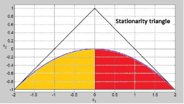
(16) Figure 5: AR(2) regression coefficients for each time series; one-lag parameter value (1 ) on the horizontal axis and two-lag parameter value (2 ) on the vertical axis. The existence or not of a computable cycle is determined by the position of the points with respect to the parabola. The Upper and Lower curves represent a 95% confidence interval as equal to twice the average standard error of the 1 and 2 estimators. The straight line represents the upper limit of the stationarity triangle. 3.3.2. Admissible area. Another possibility is that the test I am conducting is not specified correctly because I am examining only one quarter of the entire possible graph when arguing that the unconditional probability of finding a cycle is 66% over the admissible region. Technically, AR(2) regression results can yield values that do not lie in the area I have examined so far (a draw in the region delimited by 1 ∈ [−2 0] and 2 ∈ [0 1] is technically. possible). Looking at Figure 6,26 we see that a cycle will exist provided that draws are under the parabola,. whereas the AR(2) model is stationary if the draws fall within the triangle with summits (0,1), (-2,-1) and (2,-1) in the 1 , 2 space. Assuming we are only looking at the draws that yield a cycle over the entire region 1 ∈ [−2 2] and 2 ∈ [−1 1], the probability of falling in the region below the parabola with 1  0 is 1/6, or 17%. Assuming we only concentrate on draws where 1  0 − as the insurance economic literature has done − the odds of finding a cycle are 1/3. This is still quite high given the actual evidence in the data where less than one third b and  b estimators significantly different from zero using a Bonferroni or of the regressor pairs have both  1 2. a Student test. 26 I. am grateful to Richard Peter for providing me with this figure.. 14.

(17) Figure 6: Stationarity triangle and cycle parabola in an AR(2) regression.. 4. Conclusion "There is a universal tendency among mankind to conceive all beings like themselves, and to transfer to every object those qualities with which they are familiarly acquainted, and of which they are intimately conscious. We find human faces in the moon, armies in the clouds; and by a natural propensity, if not corrected by experience and reflection, ascribe malice and good will to everything that hurts or pleases us." David Hume (Natural History of Religion, Section 3, 1757).27 The purpose of this short article was to offer a challenge to the popular view that the property and casualty. insurance industry is characterized by profitability cycles akin to real business cycles in the economy. Using a meta-analysis of the, arguably, most influential papers in the field that span different lines of insurance, different countries, different samples and different AR(2) specifications, the results of the paper show that the existence of underwriting cycles is far from obvious. When a proper statistical test on the AR(2) regression parameter values is conducted (a Bonferroni test to be exact, or a more stringent Student test), I find that a cycles is likely observed in less than a quarter of the studies on the topic. This is far from the 65% to 70% likelihood that is generally presented in the literature. And even this generally reported probability range is close to the probability of finding a cycle by drawing randomly the two AR(2) parameters from a uniform distribution. 2 7 Source:. http://etyman.wordpress.com/2010/01/29/apophenia/ (last visited on 29 october 2012). 15.

(18) Of course, the analysis I present is based on results that have already been published in the literature, without verifying directly the validity of these regression results. Also, I did not use all the results that could have been found in the insurance economic literature; I only used what appeared to me to be the most influential results and those that provided estimates of the standard errors of the AR(2) regression parameters. Where does that take us in terms of research on the topic of underwriting cycles? To paraphrase the character of Ebby Calvin "Nuke" LaLoosh in the movie Bull Durham: "Sometimes profits go up; sometimes profits go down; and sometimes it rains". To be honest, it is still possible that insurance profitability cycles exist in some lines, countries and for some time period. As a whole, however, the evidence is just not there statistically and scientifically (see also Venezian, 2010, and Powers, 2012). And even if there are instances where the absence of a cycle can be rejected, there is no evidence whatsoever that the gradient of the cycle would be predictable (see Boyer et al., 2012, for more on this topic). This means that insurers that "have simply accepted the insurance cycle, seeing it as a force of nature with an uncontrollable impact on their business"28 might have been doing the right thing... inasmuch as cycles in equity index prices29 are a force of nature that have an uncontrollable impact on the design of a pension plan. The human tendency of trying to find pattern in randomness may explain why insurance economists have been trying to find explanation for the apparent cyclicality of insurer profitability. This human bias is normal, and has led many economists to develop what is now known as behavioral theories of economic life. McFadden (1999) writes "Tune (1964) and Kahneman and Tversky (1972) document experimentally that individuals intuitively reject randomness when they see recognizable patterns or streaks, systematically underestimating the probability that these can occur by chance. These biases reinforce the influence of random coincidences on beliefs and behavior" (p.93). Even though such a bias may be normal, it should not represent the basis of scientific analysis. The belief that underwriting cycles exist leads to the perception that the insurance market is plagued with imperfections. As such, the presence of underwriting cycles can become the basis of government intervention (see Gron, 2010), or can be part of a financial stability regulation to control insolvency (see Trufin et al., 2009, and European Commission, 2002) even though Winter (1991) shows that solvency regulation may actually exacerbate cycles. Perhaps we would be wise to heed the conclusion of Baker (2005) who argues 2 8 http://www.lloyds.com/Lloyds/Press-Centre/Press-Releases/2006/12/Seven_steps_to_managing_the_cycle 2 9 Using monthly data, we can calculate a cycle period of 4.69 months for total returns on the SNP500 from April 1993 until June 2012 (or 7.22 years when using yearly total return over the same period), a cycle of 4.15 months for the total returns on the FTSE100 from July 1984 until June 2012, and a cycle of 4.16 months for the total return on the 30 year treasury bond from May 1977 until June 2012.. 16.

(19) that "leaving the insurance cycle alone would be the wiser course for now". As I show in this paper, there is really no scientific (or statistical) basis to support the perception that there are profitability cycles in the property and casualty insurance industry; it is simply not there! We can therefore affirm that there is no market-wide evidence that insurance companies are behaving noncompetitively; or at least, there is no evidence that insurer profitability is not as random as what one would expect to see in a competitive market open to new entrants.. 17.

(20) 5. References 1. Alkemper, J. and D.F. Mango (2005). Concurrent Simulation to Explain Reinsurance Market Price Dynamics. Risk Management 6:13-17. 2. Baker, T. (2005). Medical Malpractice and the Insurance Underwriting Cycle. DePaul Law Review, 54.: 3. Baranoff, D. (2003). A policy of cooperation: the cartelisation of American fire insurance, 1873—1906. Financial History Review, 10: 119-136 4. Berger, L.A. (1988). A Model of the Underwriting Cycle in the Property/Liability Insurance Industry. Journal of Risk and Insurance, 55: 298-306. 5. Berger, L, J.D. Cummins and S. Tennyson (1992). Reinsurance and the Liability Insurance Crisis. Journal of Risk and Uncertainty, 5: 253-72. 6. Born, P. and W.K. Viscusi (2006). The catastrophic effects of natural disasters on insurance markets. Journal of Risk and Uncertainty 33:55—72. 7. Boyer, M.M., J. Eisenmann and J.-F. Outreville (2011). Underwriting Cycles and Underwriter Sentiment. MRIC Behavioral Insurance Conference. 8. Boyer, M.M., E. Jacquier and S. Van Norden (2012). Are Underwriting Cycles Real and Forecastable?. Journal of Risk and Insurance 79: 995—1015. 9. Brocket, P. and R.C. Witt (1982). The Underwriting Risk and Return Paradox Revisited. Journal of Risk and Insurance, 49: 621-627. 10. Carroll, R.T. (2003). The Skeptic’s Dictionary: A Collection of Strange Beliefs, Amusing Deceptions, and Dangerous Delusions. John Wiley & Sons.. 11. Chen, R., K. Wong and H. Lee (1997). Underwriting Cycles in Asia. Journal of Risk and Insurance 66: 29-47. 12. Clark, D. (2010). Understanding and projecting the U/W cycle. CAS Presentation, (cited in Wang et al. 2010) http://www.casact.org/education/reinsure/2010/handouts/CS22-Clark.pdf 13. Cummins, J.D. (2006). Should the Government Provide Insurance for Catastrophes? Federal Reserve Bank of St. Louis Review, 88: 337-379. 14. Cummins, J.D. and P.M. Danzon (1997). Price, Financial Quality, and Capital Flows in Insurance Markets. Journal of Financial Intermediation, 6: 3-38. 18.

(21) 15. Cummins, J.D. and N.A. Doherty (2002). Capitalization of the Property-Liability Insurance Industry: Overview. Journal of Financial Services Research, 21: 5-14. 16. Cummins, J.D. and J.F. Outreville (1987). An International Analysis of Underwriting Cycles. Journal of Risk and Insurance, 54: 246-262. 17. Derien, A. (2008). An Empirical Investigation of the Factors of the Underwriting Cycles in Non-Life Market. Proceedings of MAF 2008: International Conference Mathematical and Statistical Methods for Actuarial Sciences and Finance (http://maf2008.unive.it/viewpaper.php?id=46). 18. Doherty, N.A. and J.R. Garven (1992). Insurance Cycles: Interest Rates and the Capacity Constraint Model. Journal of Business, 68: 383-404. 19. Doherty, N.A. and H.B. Kang (1988). Interest Rates and Insurance Price Cycles. Journal of Banking and Finance, 12: 199-214. 20. European Commission (2002). Study into the methodologies to assess the overall financial position of an insurance undertaking from the perspective of prudential supervision. Contract no: ETD/2000/BS3001/C/45 21. Fields, J.A. and E.C. Venezian (1989). Interest Rates and Profit Cycles: A Disaggregated Approach. Journal of Risk and Insurance 56: 312-319. 22. Fitzpatrick, S.M. (2004). Fear is the Key: A Behavioral Guide to Underwriting Cycles. Connecticut Insurance Law Journal, 10(2): 255-275. 23. Gron, A. (1994a). Evidence of Capacity Constraints in Insurance Markets. Journal of Law and Economics, 37: 349-377. 24. Gron, A. (1994b). Capacity Constraints and Cycles in Property-Casualty Insurance Markets. RAND Journal of Economics. 25: 110-127. 25. Gron, A. (2010). Insurance Price and Profit Dynamics: Underwriting Cycles Can Occur in Competitive Markets. American Bar Association Spring 2010 Section of Antitrust Law. 26. Hamilton, J.D. (1994). Time Series Analysis. Princeton University Press, Princeton. 27. Harrington, S.E. (2004). Tort Liability, Insurance Rates, and the Insurance Cycle. Brookings-Wharton Papers on Financial Services, pp. 97-138. 28. Harrington, S.E. and P.M. Danzon (1994). Price Cutting in Liability Insurance Markets. Journal of Business, 67: 511-538. 19.

(22) 29. Harrington, S.E. and G. Niehaus (2000). Volatility and Underwriting Cycles. In G. Dionne (editor), Handbook of Insurance, Kluwer Academic Publishers, pages 657—686. 30. Harrington, S.E., and T. Yu (2003). Do Property-Casualty Insurance Underwriting Margins Have Unit Roots? Journal of Risk and Insurance 70: 715—733. 31. Hartwig, R.P. (2011). Is the World Becoming a Riskier Place? Economic Overview and P/C Insurance Industry Outlook for 2012 & Beyond. Insurance Information Institute, (www.iii.org/presentations). 32. Jarque, C.M. and A.K. Bera (1980). Efficient Tests for Normality, Homoscedasticity and Serial Independence of Regression Residuals. Economics Letters 6: 255-259. 33. Kahneman, D. and A. Tversky (1972). Subjective Probability: A Judgment of Representativeness. Cognitive Psychology, 3: 430-451. 34. Lamm-Tennant, J., L.T. Starks and L. Stokes (1992). An Empirical Bayes Approach to Estimating Loss Ratios. Journal of Risk and Insurance, 59: 426-442. 35. Lamm-Tennant, J. and M.A. Weiss (1997). International Insurance Cycles: Rational Expectations/Institutional Intervention. Journal of Risk and Insurance 64: 415-439. 36. Lloyd’s (2006). Annual Report - Strategy. 37. Lloyd’s (2007). Annual Underwriter Survey. 38. McFadden, D. (1999). Rationality for Economists? Journal of Risk and Uncertainty 19:73-105 39. McKinsey & Company (2008). Managing Through the P&C Cycle. Working Paper authored by T. Catlin, J. Peters and P. Walker. 40. Meier, U.B. (2006a). Multi-national underwriting cycles in property-liability insurance: Part 1. Journal of Risk Finance 7: 64-82. 41. Meier, U.B. (2006b). Multi-national underwriting cycles in property-liability insurance: Part 2. Journal of Risk Finance 7: 83-97. 42. Meier, U.B. and J.-F. Outreville (2006). Business Cycle in Insurance and Reinsurance: The Case of France, Germany and Switzerland. Journal of Risk Finance 7: 160-176. 43. Nelson, C. R., and C.I. Plosser (1982). Trends and Random Walks in Macroeconomic Time Series: Some Evidence and Implications. Journal of Monetary Economics 10: 139-162.. 20.

(23) 44. Niehaus, G. and A. Terry (1993). Evidence on the Time Series Properties of Insurance Premiums and Causes of the Underwriting Cycle: New Support for the Capital Market Imperfection Hypothesis. Journal of Risk and Insurance, 60: 466-479. 45. Outreville, J.F. (1990). Underwriting Cycles and Rate Regulation In Automobile Insurance Markets. Journal of Insurance Regulation, 9: 274-286. 46. Powers, M. (2012). Acts of God and Man, Columbia University Press, New York. 47. Sargent, T. (1986). Macroeconomic Theory, Academic Press, New York, 2nd Edition. 48. Shapiro, S.S. and M.B. Wilk (1965). An Analysis of Variance Test for Normality (Complete Samples). Biometrika 52: 591-611. 49. Sterman, J.D. (1994). Learning in and about complex systems. System Dynamics Review, 10: 291—330. 50. Stewart, B.D. (1981, 1984). Profit Cycles in Property-Liability Insurance. In Issues in Insurance, Vol. 2, edited by J.B. Long, Malvern, Pa. 51. Stock, J. and M. Watson (1988). Variable Trends in Economic Time Series. Journal of Economic Perspectives 2: 147-174. 52. Tarr, F. (2008). An investigation into the existence of Underwriting Cycles in the South African Primary Marine Insurance Market: 1925-2006. Unpublished thesis, University of the Witwatersrand, Johannesburg. 53. Trufin, J., H. Albrecher and M. Denuit (2009). Impact of Underwriting Cycles on the Solvency of an Insurance Company. North American Actuarial Journal, 13: 385-403. 54. Tune, G. (1996). Neglect of Stimulus Information in a Two-choice Task. Journal of General Psychology, 74: 231-236 55. Venezian, E. (1985). Rate making Methods and Profit Cycles in Property and Liability Insurance. Journal of Risk and Insurance 52: 477-500. 56. Venezian, E. (2006). The use of spectral analysis in insurance cycle research. Journal of Risk Finance, 7: 177-188. 57. Venezian, E. and C.-C. Leng (2006). Application of spectral and ARIMA analysis to combined-ratio patterns. Journal of Risk Finance, 7: 189-214. 58. Wang, S.S., J.A. Major, C.H. Pan and J.W.K. Leong (2010). Underwriting Cycle Modeling and Risk Benchmarks. Joint Research Paper of Risk Lighthouse LLC and Guy Carpenter & Company, LLC. 21.

(24) 59. Wilson, W.C. Jr. (1981). The Underwriting Cycle and Investment Income. CPCU Journal, 34: 225-232. 60. Winter, R.A. (1991). The Liability Insurance Market. Journal of Economic Perspective 5: 115—136. 61. Winter, R.A. (1994). The Dynamics of Competitive Insurance Markets. Journal of Financial Intermediation 3: 279-315. 62. Zanjani, G. (2004). Mutuality and the Underwriting Cycle: Theory with Evidence from the Pennsylvania Fire Insurance Market, 1873-1909. Mimeograph, Federal Reserve Bank of New York, available at SSRN: http://ssrn.com/abstract=519603. 63. Zellner, A. (1971). An Introduction to Bayesian Inference in Econometrics. New York : Wiley.. 22.

(25) 6. Appendix 0,800 0,600 0,400. Harrington & Niehaus. 0,200 0,000 0,000. 0,200. 0,400. 0,600. 0,800. 1,000. 1,200. 1,400. 1,600. 1,800. 2,000. ‐0,200. Venezian ‐0,400 ‐0,600. Chen ‐0,800 ‐1,000. Cummins & Outreville Problematic. Less Problematic. Figure 7: AR(2) regression coefficients for each time series; one-lag parameter value (1 ) on the horizontal axis and two-lag parameter value (2 ) on the vertical axis. Some datapoint sources (3 of 25 from Chen et al., 1997, 6 of 20 from Cummins and Outreville, 1987, 8 of 12 from Venezian, 1985, and 3 of 6 from Harrington and Niehaus, 2000) are indicative of some level of clustering of the 1 and 2 regression results.. 23.

(26)