How Much Inflation is Necessary to Grease the Wheels?

2007-10

Kim, Jinill

Ruge-Murcia, Francisco J.

How Much Inflation is Necessary

to Grease the Wheels?

Département de sciences économiques Université de Montréal

Faculté des arts et des sciences C.P. 6128, succursale Centre-Ville Montréal (Québec) H3C 3J7 Canada http://www.sceco.umontreal.ca SCECO-information@UMontreal.CA Téléphone : (514) 343-6539 Télécopieur : (514) 343-7221

Ce cahier a également été publié par le Centre interuniversitaire de recherche en économie quantitative (CIREQ) sous le numéro 11-2007.

This working paper was also published by the Center for Interuniversity Research in Quantitative Economics (CIREQ), under number 11-2007.

How Much In ation is Necessary

to Grease the Wheels?

Jinill Kim

Federal Reserve Board

Jinill.Kim@frb.gov

Francisco J. Ruge-Murcia

University of Montreal

francisco.ruge-murcia@umontreal.ca

September 2007

This paper studies Tobin's proposition that in ation \greases" the wheels of the labor market. The analysis is carried out using a simple dynamic stochastic general equilibrium model with asymmetric wage adjustment costs. Optimal in ation is de-termined by a benevolent government that maximizes the households' welfare. The Simulated Method of Moments is used to estimate the nonlinear model based on its second-order approximation. Econometric results indicate that nominal wages are downwardly rigid and that the optimal level of grease in ation for the U.S. economy is about 1.2 percent per year, with a 95% con dence interval ranging from 0.2 to 1.6 percent.

JEL Classi cation: E4, E5.

Key Words: Optimal in ation, asymmetric adjustment costs, nonlinear dynamics.

We received helpful comments and suggestions from Michelle Alexopoulos, Gauti Eggertsson, Steinar Holden, and Junhan Kim. The rst author thanks CIREQ and the Department of Economics of the University of Montreal for their hospitality. This research received the nancial support of the Social Sciences and Humanities Research Council of Canada. Correspondence to: Francisco J. Ruge-Murcia, Departement de sciences economiques, Universite de Montreal, C.P. 6128, succursale Centre-ville, Montreal (Quebec) H3C 3J7, Canada.

1

Introduction

In his presidential address to the American Economic Association in 1971, James Tobin suggests that a positive rate of in ation may be socially bene cial in an economy where nominal prices|in particular, nominal wages|are more downwardly rigid than upwardly rigid (Tobin, 1972). To illustrate Tobin's argument, suppose that the economy is hit by an exogenous shock that requires a decline in the real wage, such as a negative productivity shock. Two plausible adjustment paths are to keep the price level xed and cut nominal wages, and to keep the nominal wages xed and increase the price level. Tobin claims that the former path, which is characterized by a zero in ation rate, may involve signi cant social costs when nominal wages are downwardly rigid. Instead, the latter path, which features a positive in ation rate, may deliver the same reduction in the real wage at a lower cost. The idea that in ation eases the adjustment of the labor market by speeding the decline of real wages following an adverse shock is described in the literature by the catchphrase that in ation \greases the wheels of the labor market."

This paper uses a stylized dynamic stochastic general equilibrium model with asymmetric nominal rigidities to formally examine Tobin's proposition and to construct a theory-based estimate of the optimal amount of \grease" in ation for the U.S. economy. Optimal in ation is determined in our model by a benevolent government that maximizes the households' welfare under commitment (i.e., the Ramsey policy). A nonlinear approximation of the model is estimated by the Simulated Method of Moments and an estimate of optimal grease in ation is constructed by measuring how much more expected in ation asymmetric costs yield compared to symmetric costs.

This subject matter is important because there is currently a discrepancy between eco-nomic theory|that prescribes a zero-to-negative optimal in ation rate|and monetary pol-icy in practice|that explicitly or implicitly targets low, but strictly positive, in ation rates. The theoretical result that optimal in ation is negative is driven by Friedman's rule (Fried-man, 1969). Under Friedman's rule a rate of de ation equal to the real return on capital eliminates the wedge between social marginal cost of producing money, which is essentially zero, and the private marginal cost of carrying money, which is the nominal interest rate. Additional considerations like scal policy and price rigidity, deliver optimal in ation rates that are larger than Friedman's rule but still negative.1

1_{See, among many others, Rotemberg and Woodford (1997), Chari and Kehoe (1999), Teles (2003), Khan,}

King and Wolman (2003), Kim and Henderson (2005), and Schmitt-Grohe and Uribe (2004, 2006), as well as references therein. In addition to the asymmetric nominal rigidities studied here, another reason because of which optimal in ation may be positive is the zero lower-bound on nominal interest rates (see, for example, Billi, 2005).

The idea that wages are more downwardly (than upwardly) rigid dates at least to Keynes (1936, Chapter 21). Empirical evidence on downward wage rigidity using micro-level data takes the form of attitude surveys and the empirical analysis of wage distributions. Bewley (1995) and Campbell and Kamlani (1997) nd that employers cut wages only in cases of ex-treme nancial distress while worrying about the e ect of nominal wage cuts on the worker's morale. Kahneman, Knetsch and Thaler (1986) nd that individuals dislike nominal wage cuts more than an alternative scenario even when both of them involve the same real wage cut. Researchers who study the distribution of nominal wage changes at the individual level point out that it features a peak at zero and is positively skewed with very few nominal wage cuts. See, for example, McLaughlin (1994), Akerlof et al. (1996), and Card and Hyslop (1997) for the United States; Kuroda and Yamamoto (2003) for Japan; Castellanos et al. (2004) for Mexico; and Fehr and Goette (2005) for Switzerland. Institutional characteristics, like laws forbidding nominal wage cuts (Mexico) or making the current nominal wage the default outcome when union-employer negotiations fail, may also contribute to downward nominal wage rigidity.

This paper reports four main results. First, U.S. prices and wages are rigid, but in the case of wages, rigidity is asymmetric in the sense that they are more downwardly rigid. This conclusion is based on an econometric estimate of the asymmetry in the wage adjustment cost function. Second, the Ramsey policy prescribes a positive (gross) rate of price in ation of about 1.012 (i.e., optimal grease in ation of about 1.2 percent per year). This result is driven by prudence, meaning that the benevolent planner prefers the systematic, but small, price and wage adjustment costs associated with a positive in ation rate rather than taking the chance of incurring the large adjustment costs associated with nominal wage decreases. Third, asymmetry in wage adjustment costs delivers non-trivial implications for optimal responses following a productivity shocks and generates higher-order properties that are roughly in line with those found in the U.S. data. Finally, in the case where monetary policy were implemented by a strict in ation target, the optimal target is substantially larger than the unconditional in ation mean obtained under the Ramsey policy.

The paper is organized as follows. Section 2 constructs a model with imperfect compe-tition and asymmetric price- and wage-adjustment costs and describes the Ramsey problem of the benevolent government. Section 3 presents the econometric methodology and reports estimates of the structural parameters. Section 4 reports estimates of optimal grease in a-tion, studies the dynamic implications of the model, and compares welfare under the Ramsey policy and under strict in ation targeting. Section 5 concludes and discusses current and future work in our research agenda on asymmetric nominal rigidities.

2

The Model

2.1

Households

The economy is populated by a continuum of in nitely-lived households indexed by n_{2 [0; 1] :} Households are identical, except for the fact that they have di erentiated job skills which give them monopolistically competitive power over their labor supply. At time , household n maximizes E 1 X t= (t ) (cnt)1 1 (hn t)1+ 1 + ! ; (1)

where _{2 (0; 1) is the subjective discount factor, c}n_t is consumption, hn_t is hours worked, and and are positive preference parameters.2 _{Consumption is an aggregate of di erentiated}

goods indexed by i_{2 [0; 1]} cn_t = 0 @ 1 Z 0 (cn_i;t)1= di 1 A ; (2)

where > 1: In this speci cation, the elasticity of substitution between goods is constant and equal to =( 1). When _{! 1, goods become perfect substitutes and the elasticity} of substitution tends to in nity. When _{! 1; the aggregator becomes the Cobb-Douglas} function and the elasticity is unity.

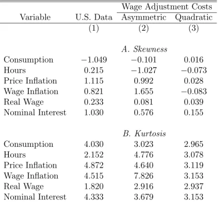
As monopolistic competitors, households choose their wage and labor supply taking as given the rms' demand for their labor type. Labor market frictions induce a cost in the adjustment of nominal wages. This cost takes the form of the linex function (as introduced by Varian, 1974) n t = (Wtn=Wt 1n ) = 0 @exp W n t=Wt 1n 1 + Wtn=Wt 1n 1 1 2 1 A; (3) where Wn

t is the nominal wage, and and are cost parameters. This functional form

is attractive for four reasons. First, the cost depends on both the magnitude and sign of the wage adjustment. Consider, for example, the case where > 0: As W_tn increases over W_{t 1}n , the linear term dominates and the cost associated with wage increases rises linearly. In contrast, as Wn

t decreases below Wt 1n ; it is the exponential term that dominates and the cost

2_{In preliminary work, we studied a more general formulation with aggregate shocks to the disutility of}

work and to the overall level of utility. However, results were very similar to the ones reported here. The shock to the disutility of work behaves like the productivity shock speci ed in Section 2.2 but its estimated conditional variance was much smaller. The shock to the level of utility disturbs the household's Euler equation for consumption, but the Ramsey planner would adjust the nominal interest rate to perfectly undo this shock's e ects. Hence, decision rules for all variables (except for the nominal interest rate) would be independent of the shock.

associated with wage decreases rises exponentially. Hence, nominal wage decreases involve a larger frictional cost than increases, even if the two percentage magnitudes are the same. The converse is true in the case where < 0. Second, the function nests the quadratic form as a special case when tends to zero.3 _{Thus, the comparison between the model with}

asymmetric costs and a restricted version with quadratic costs is straightforward. Third, the linex function is di erentiable everywhere and strictly convex for any > 0: Finally, this function does not preclude nominal wage cuts that, although relatively rare, are observed in micro-level data. In order to develop further the readers' intuition, Figure 1 plots the quadratic and asymmetric cost functions, the latter in the case of a positive .

There are two types of nancial assets: one-period nominal bonds and Arrow-Debreu state-contingent securities. The household enters period t with Bt 1 nominal bonds and

a portfolio At 1 of state-contingent securities, and then receives wages, interests, dividends

and state-contingent payo s. These resources are used to nance consumption and the acquisition of nancial assets to be carried out to the next period. Expressed in real terms, the household's budget constraint is

cn_t + t;t+1A n t Ant 1 Pt +B n t It 1Bt 1n Pt = W n t hnt Pt ! (1 n_t) + D n t Pt ;

for t = ; + 1; : : : ;_{1, where} t;t+1 is a vector of prices, It is the gross nominal interest rate,

Dn_t are dividends and

Pt= 0 @ 1 Z 0 (Pi;t)1=(1 )di 1 A 1=(1 ) ; (4)

is an aggregate price index with Pi;t denoting the price of good i. Without loss of generality,

it is assumed that the wage adjustment cost is paid by the household. Prices are measured in terms of a unit of account called \money," but the economy is cashless otherwise.

The household's utility maximization involves choosing _fcn_t; An_t; B_tn; W_tn; hn_tg1_t= subject to the initial asset holdings and the sequence of wages, labor demand, budget constraints, and a no-Ponzi-game condition. First-order necessary conditions include

(ct) = t; (5)

whereby the marginal utilities wealth and consumption are equalized at the optimum, and

t Pt 1 ! hn_t (1 n_t) + W n t Wn t 1 ! hn_t ( n_t)0 ! (6) = t Pt (hn_t (1 n_t)) + 1 (hn t)1+ Wn t ! + Et 0 @ t+1 Pt+1 W_t+1n Wn t !2 hn_t+1 n_t+1 0 1 A;

3_{To see this, take the limit of}

where =( 1) is the elasticity of substitution between labor types (as speci ed below in the rms' problem), and ( n

t)0 denotes the derivative of the cost function with respect to

its argument.4 _{Condition (6), usually referred to as the wage Phillips curve, equates the}

marginal costs and bene ts of increasing Wn

t : The costs are the decrease in hours worked as

rms substitute away from the more expensive labor input, and the wage adjustment cost. The bene ts are the increase in labor income per hour worked, the increase in leisure time as rms reduce their demand for type-n labor, and the reduction in the future expected wage adjustment cost. Given nominal consumption expenditures, the optimal consumption of good i satis es cn_i;t = Pi;t Pt =( 1) cn_t: (7)

2.2

Firms

Each rm produces a di erentiated good i _{2 [0; 1] using a production function featuring} decreasing returns to scale,

yi;t = xth1i;t ; (8)

where yi;t is output of good i, hi;t is labor input, 2 (0; 1] is a production parameter, and xt

is an exogenous productivity shock. The productivity shock follows the stochastic process ln(xt) = ln(xt 1) + "t;

where _{2 ( 1; 1) and "}t is an identically and independently distributed innovation with

zero mean and variance 2_{. Labor input is an aggregate of heterogeneous labor supplied by}

households, hi;t = 0 @ 1 Z 0 (hn_i;t)1= dn 1 A ; (9)

where > 1: The price of the labor input is

Wi;t = 0 @ 1 Z 0 (W_tn)1=(1 )dn 1 A 1 ; (10)

where W_tn is the wage demanded by the supplier of type-n labor. Product di erentiation gives the rm monopolistically competitive power, so price is a choice variable. However,

4_{The other rst-order conditions (not shown) price the nominal bond and the portfolio of state contingent}

the adjustment of nominal prices is assumed to be costly. In particular, the real cost of a price change per unit is

i

t = (Pi;t=Pi;t 1) =

exp( & (Pi;t=Pi;t 1 1)) + & (Pi;t=Pi;t 1 1) 1

&2

!

; (11) where (> 0) and & are cost parameters. In what follows, we focus on the special case where & _{! 0 (i.e., the quadratic cost function proposed by Rotemberg, 1982) and price adjustment} costs are, therefore, symmetric.5

At time ; rm i maximizes the discounted sum of real pro ts

E 1 X t= (t ) t Pt 0 @ 1 i_t Pi;tci;t 1 Z 0 W_tnhn_tdn 1 A; and ci;t = 1 R 0 cn

i;tdn is total consumption demand for good i. Maximization is subject to the

technology (8), the downward-sloping consumption demand function (7), and the condition that supply must meet the demand for good i at the posted price. First-order conditions equate the marginal productivity of labor with its cost,

(1 )xthi;t = Wi;t=Pi;t; (12)

and the marginal costs with the marginal bene ts of increasing Pi;t;

1 Pt 1 ! ci;t 1 it + Pi;t Pi;t 1 ! ci;t it 0! (13) = 1 Pt ci;t 1 it + 1 tyi;t Pi;t ! + Et 0 @ t+1 t ci;t+1 Pt+1 Pi;t+1 Pi;t !2 i t+1 0 1 A;

where tis the nominal marginal cost. On the left-hand side of this price Phillips curve, the

costs are the decrease in sales, which is proportional to the elasticity of substitution between goods, and the price adjustment cost. On the right-hand side, the bene ts are the increase in revenue for each unit sold, the decrease in the marginal cost, and the reduction in the

5_{In preliminary work, we considered an unrestricted version of the model with a possibly non-zero &.}

However, a Wald test of & = 0 does not reject this hypothesis at the 5 percent signi cance level, and identi cation of the other parameters is considerably sharper when this restriction is imposed. Peltzman (2000) studies the pricing decisions of a Chicago supermarket chain at the level of individual goods and nds no asymmetry in its response to input price increases or decreases. Zbaracki et al. (2004) nds that customers are antagonized by price changes, even when they involve a price decrease. Price decreases are not always welcomed because passing lower prices downstream also involves adjustment costs and because current price cuts make future price increases more costly (see p. 527). In summary, the data seem to be in reasonable agreement with the assumption that price adjustment costs are symmetric.

future expected price adjustment cost. Given nominal expenditures on labor, the optimal demand of type-n labor is

hn_t = W n t Wt =( 1) ht

where =( 1) is the elasticity of demand for the labor of household n with respect to its relative wage.

2.3

Symmetric Equilibrium

In the symmetric equilibrium, all households supply exactly the same amount of labor. This implies that hn_t = htand, consequently, Wtn= Wt: Since households are identical in all

other respects, it follows that their equilibrium choices will be same, that n subscripts can be dropped without loss of generality, and that net holdings of Arrow-Debreu securities and bonds can be neglected in the solution. Similarly, all rms are identical ex-post meaning that they charge the same price and produce the same quantity. Hence, all relative prices are one and the i subscripts can also be dropped. Substituting the government's budget constraint and the pro ts of the (now) representative rm into the budget constraint of the (now) representative household delivers the economy-wide resource constraint:

ct= yt(1 t) wtht t: (14)

where wt = Wt=Pt is the real wage.

2.4

Monetary Policy

The government follows a Ramsey policy of maximizing the households' welfare subject to the resource constraint while respecting the rst-order conditions of rms and households.6

That is, the government chooses _fct; t; ht; wt; it; t; tg1t= to maximize

E 1 X t= (t ) (ct)1 1 (ht)1+ 1 + ! ;

where t = Wt=Wt 1 is gross wage in ation and t= Pt=Pt 1is gross price in ation, subject

to conditions (5), (6), (12), and (13), and taking as given previous values for wages, goods prices, and shadow prices. Notice that in the formulation of the government's problem, it is assumed that the discount factor used to evaluate future utilities is the same as that used

6_{Admittedly, the Ramsey policy is an incomplete characterization of U.S. monetary policy. However,}

this policy|unlike ad-hoc policy rules|endogenously determines the behavior of the government, including the deterministic steady state for in ation. In Section 4.4, we compare the outcomes of the Ramsey policy with those of a simple in ation targeting rule

by households.7 _{It is also assumed that the government can commit to the implementation}

of the optimal policy.

Since this problem does not have a closed-form solution, we use a perturbation method that involves taking a second-order Taylor series expansion of the government's decision rules as well as its constraints and characterizing local dynamics around the deterministic steady state. See Jin and Judd (2002), Kim, Kim, Schaumburg and Sims (2003), and Schmitt-Grohe and Uribe (2004) for a detailed explanation of this approach.8

3

Estimation

3.1

Data

The data used to estimate the model are quarterly observations of the real wage, hours worked, real consumption per capita, the price in ation rate, the wage in ation rate, and the nominal interest rate between 1964Q2 to 2006Q2. The sample starts in 1964 because aggregate data on wages and hours worked are not available prior to that year. The raw data were taken from the database available at the Federal Reserve Bank of St. Louis. The rates of price and wage in ation are measured by the percentage change in the Consumer Price Index (CPI) and the average hourly earnings for private industries. Hours worked is the total number of weekly hours worked in private industries. The nominal interest rate is the three-month Treasury Bill rate. Real consumption is measured by the Personal Consumption Expenditures in nondurable goods and services per capita divided by the CPI. The population series corresponds to the quarterly average of the mid-month U.S. population estimated by the Bureau of Economic Analysis (BEA). Except for the nominal interest rate, all data are seasonally adjusted at the source. All series were logged and linearly detrended prior to the estimation of the model.

3.2

Econometric Methodology

The second-order approximate solution of our nonlinear DSGE model is estimated using the Simulated Method of Moments (SMM). The application of SMM for the estimation

7_{In preliminary work, we relaxed this assumption and estimated the government's discount factor}

sepa-rately from that of households. However, econometric estimates were remarkably similar and di ered only after the fth decimal. It is interesting to note that when both factors are assumed to be di erent, the iden-ti caiden-tion of the wage asymmetry parameter is sharper because in this case this parameter a ects rst-order dynamics.

8_{The codes that we employed were adapted from those originally written by Stephanie Schmitt-Grohe}

and Martin Uribe. The dynamic simulations of the nonlinear model are based on the pruned version of the model, as suggested by Kim, Kim, Schaumburg and Sims (2003).

of time-series models was proposed by Lee and Ingram (1991) and Du e and Singleton (1993). Ruge-Murcia (2007) uses Monte-Carlo analysis to compare various methods used for the estimation of DSGE models and reports that moment-based estimators are gener-ally more robust to misspeci cation than Maximum Likelihood (ML). This is important because economic models are stylized by de nition and misspeci cation of an unknown form is likely.9 _{Method of Moments estimators are also attractive for the estimation of nonlinear}

DSGE models because the numerical evaluation of its objective function is relatively cheap. This means, for example, that the researcher can a ord to use genetic algorithms for its optimization. These algorithms require a larger number of function evaluations than alter-native gradient-based methods, but greatly reduce the possibility of converging to a local optimum|rather than the global one.

De ne to be a q 1 vector of structural parameters, gtto be a p 1 vector of empirical

observations on variables whose moments are of our interest, and g ( ) to be the synthetic counterpart of gt whose elements come from simulated data generated by the model. Then,

the SMM estimator, b; is the value that solves min f g G( ) 0_{WG( ); (15)} where G( ) = (1=T ) T X t=1 gt (1= T ) T X =1 g( );

T is the sample size, is a positive constant, and W is a q q weighting matrix. Under the regularity conditions in Du e and Singleton (1993),

p T (b )_{! N(0;(1 + 1= )(D}0W 1D) 1D0W 1SW 1D(D0W 1D) 1); (16) where S= lim T !1V ar (1= p T ) T X t=1 gt ! ; (17)

and D = E(@g ( )=@ ) is a q p matrix assumed to be nite and of full column rank.10

9_{On the other hand, under the assumption that the model is correctly speci ed, ML is statistically more}

e cient than the Method of Moments. This means that, even though both methods deliver consistent parameter estimates, those obtained by ML would typically have smaller standard errors.

10_{An alternative approach is to analytically compute the moments predicted by the model based on the}

pruned quadratic solution and use them in the objective function instead of (1= T )

T

P

=1

g( ): We followed this GMM approach in preliminary work but found it problematic because, under the assumption that the private and social discount factors are the same, rst-order dynamics are independent of the asymmetry parameter, and, consequently, is not identi ed. Notice that for the pruned version of nonlinear DSGE models, SMM is not statistically equivalent to GMM as _{! 1. In contrast, the two are asymptotically} equivalent in the case of linear models (see Ruge-Murcia, 2007)

In this application, contains the discount factor ( ), the curvature parameters of the utility function ( and ), the parameters of the adjustment cost function ( ; and ), and the parameters of the productivity shock process ( and ). For the simulation of the model, the productivity innovations are drawn from a Normal distribution.11 _The

weighting matrix W is the diagonal of the inverse of the matrix with the long-run variance of the moments, S: In turn, S is computed using the Newey-West estimator with a Barlett kernel. The derivatives in the Jacobian matrix D are numerically computed at the optimum. The moments in G( ) are ve (out of six) variances, all twenty one covariances and all six autocovariances of the data series.12

Three parameters are weakly identi ed in the initial estimation and, consequently, we use additional information to x their values to economically plausible numbers during the estimation routine. These parameters are the curvature of the production function (1

) and the elasticities of substitution between goods and between labor types ( and , respectively). Data from the U.S. National Income and Product Accounts (NIPA) show that the share of labor in total income is approximately 2/3 and, therefore, a plausible value for is 1/3. The elasticities of substitution between goods and between labor types are xed to = 1:1 and = 1:4; respectively. This value for is standard in the literature. Sensitivity analysis with respect to indicates that results are robust to using similarly plausible values.

3.3

SMM Estimates

SMM parameter estimates based on the second-order approximate solution of the model are reported in the rst column of Table 1. Regarding the preference parameters, notice that the coe cient that determines the consumption curvature ( ) is statistically di erent from zero but not from one at the 5 percent signi cance level. Since, in addition, its point estimate is quantitatively very close to one, it follows that consumption preferences may

11_{We also estimated a version of the model where innovations follow a t distribution. Results are very}

similar to those reported here because the estimated number of degrees of freedom is large and the two distributions (the t and the Normal) resemble each other.

12_{The variance of the real wage is not included in G( ) because the real wage is the ratio of nominal wages}

to the CPI and so it is possible to show that

V ar(w_bt) = (1=2)(V ar( bt) + V ar(bt)) Cov( bt; bt) + Cov(wbt;wbt 1);

where the "hat" denotes deviation from the deterministic steady state. Hence, the variance of the real wage contributes no additional information beyond that contained in the variances of price in ation and wage in ation, their covariance, and the autocovariance of the real wage, all of which are included in G( ): In other words, if one were to include the variance of the real wage, then as a result of the linear combination above, the Jacobian matrix of the moments, D, would not be of full rank and regularity conditions in Du e and Singleton (1993) would not be satis ed.

be well approximated by a logarithmic function. On the other hand, the coe cient that determines the leisure curvature ( ) is quantitatively and statistically close to zero. Thus, the aggregate representation of the households' disutility of work is empirically consistent with the indivisible-labor model (Hansen, 1985).

Regarding the parameters of the adjustment cost functions, the hypotheses that = 0 and = 0 can be rejected against the respective alternatives that > 0 and > 0 at the 10 and 5 percent signi cance levels. In other words, the data rejects the hypothesis that U.S. nominal wages and prices are exible in favor of the alternative hypothesis that they are rigid. Similar results are reported, among others, by Kim (2000), Ireland (2001), and Christiano, Eichenbaum and Evans (2005) using linear DSGE models that explicitly or implicitly impose symmetry in the adjustment costs of nominal variables.

The estimate of the wage asymmetry parameter is 901:4 with a standard error of 426:2. Since this estimate of positive and statistically di erent from zero at the 5 percent level, we conclude that U.S. nominal wages are more downwardly than upwardly rigid. Returning to Figure 1, note that the parameters used to construct the asymmetric cost function are the SMM estimates reported in Table 1, that is = 33:72 and = 901:4: This gure implies, for example, that an aggregate nominal-wage cut of one percent would involve frictional adjustment costs of 0.1 percent of annual labor income, while a cut of 2 percent would involve costs of 1.4 percent. Finally, estimates of the parameters of the process of the productivity shock are very similar to those reported in earlier empirical work.

In order to examine the properties of our model, it is useful to have as benchmark a restricted version of the model with quadratic wage adjustment costs. This restricted version corresponds to the special case where _{! 0. SMM estimates of this model are} reported in the second column of Table 1. Note that the estimates of the preference and productivity parameters for this model are very similar to those reported for the asymmetric model. Estimates of the adjustment cost functions are imprecise but would tend to suggest that wages are substantially more rigid than prices. This implication of the quadratic cost model is not necessarily at odds with the data, except that results reported above in this paper would nesse this implication by noting that most of observed nominal wage rigidity is in the downward direction.

4

Properties of the Estimated Model

4.1

Optimal Grease In ation

This section constructs a measure of optimal grease in ation for the U.S. economy by cal-culating how much asymmetric costs increase expected in ation compared with symmetric (i.e., quadratic) costs. For this purpose, we compute via simulation the unconditional in ation mean implied by the two versions of our model, as reported in Table 1.

Consider rst the model with symmetric costs (the right column). The unconditional mean of annual gross in ation is 1.000012 with the 95 percent con dence interval of [1.000008, 1.000018].13 _{Since this con dence interval does not include the value of 1, the null hypothesis}

that optimal gross in ation is unity can be rejected at the 5 percent signi cance level. This result is due to the model's departure from certainty equivalence. However, given the clearly small magnitude of optimal net in ation, of about 0.12 basis points, this departure is economically insigni cant.

Consider now the model with asymmetric costs. The estimate of the unconditional mean of annual gross in ation is 1.012 with 95 percent con dence interval equal to [1.002, 1.016]. As before, this con dence interval does not include 1 and, consequently, the null hypothesis that optimal gross in ation is unity can be rejected at the 5 percent signi cance level. However, the departure from certainty equivalence in this case is not only statistically but also economically signi cant. Optimal in ation is substantially larger than 1 because the monetary authority acts prudently and reduces the probability of facing highly costly downward nominal-wage adjustment by choosing an average rate of price (and wage) in ation well above unity.

This paper de nes the measure of grease in ation as the di erence between the two gures reported above. Subtracting optimal gross in ation under the asymmetric-cost model from its corresponding value under the symmetric-cost model delivers an estimate of optimal grease in ation for the U.S. economy at approximately 0.012, that is, 1.2 percent per year. Since the con dence interval of the symmetric-cost model is very narrow and near unity, a 95 percent con dence interval for the optimal grease in ation would range roughly from 0.2 to 1.6 percent.

13_{The lower and upper bounds of this interval are computed as follows. First, we draw 120 independent}

realizations of from the empirical joint density function of the SMM estimates. Then, for each realization of , we compute the expected in ation rate. Finally, the bounds of the con dence interval are the 2:5th and 97:5th quantiles of the simulated expected in ation rates.

4.2

Impulse Responses

This section examines how the economy responds to shocks. Starting at the stochastic steady state, the economy is subjected to an unexpected temporary shock, and the responses of consumption, hours worked, price in ation, wage in ation, the real wage, and the interest rate are then plotted as a function of time. In linear models, the responses to a shock of size are one-half those to a shock size 2 and the mirror image of those to a shock of size . Thus, any convenient normalization (e.g., = 1) summarizes all relevant information about dynamics. However, in nonlinear models like ours, responses will typically depend on both the sign and the size of the shock.14 _{Thus, we plot responses to innovations of size}

+1; +2, 1, and 2 standard deviations. Responses to productivity shocks when = 0 and 901:4 are reported in Figures 2 and 3, respectively. The vertical axis is the percentage deviation from the deterministic steady state and the at line is the level of the stochastic steady state. The distance between this line and zero represents the e ect of uncertainty on the unconditional rst-moments of the variables and, thus, the model's departure from certainty equivalence.

First, consider the responses in Figure 2, where = 0: Following a negative shock, consumption, hours, wage in ation, and the real wage decrease, while price in ation and the nominal interest rate increase. The converse happens following a positive shock. There is very little asymmetry between positive and negative, and between small and large shocks.

Now, consider the responses in Figure 3, where = 901:4. A negative productivity shock decreases the marginal productivity of labor and consequently the real wage must fall. This is an example of the type of shock that Tobin had in mind in his presidential address to the American Economic Association. From Figures 2 and 3, it is apparent that the real wage does indeed fall as required but that the optimal adjustment depends on the size of the asymmetry parameter :

When = 0, the nominal wage decreases and price level increases (Figure 2). When > 0, the Ramsey policy involves positive average rates of price and wage in ation. Hence, in Figure 3, the nominal wage still increases or decreases by very little. Wage in ation is initially larger than its steady state when the shock is large and most of the reduction in the real wage is achieved by an increase in the price level. Thus, the response of price in ation is larger when > 0 than when = 0 and more than proportional when the shock is large. Hours and consumption decrease following a negative shock, and their response to a large shock of 2 is more than twice of that to a smaller shock of :

14_{See Gallant, Rossi and Tauchen (1993), and Koop, Pesaran, and Potter (1996) for more complete}

Consider also the e ect of a positive productivity shock. In this case, the real wage increases but again the adjustment depends on the value of : In general, the adjustment takes place with a decrease of the price level and an increase in the nominal wage. However, the decrease of the price level is smaller and the increase in the nominal wage is larger than in the case where = 0. This e ect increases when the productivity shock is larger. The increase of hour and consumption and the decrease in the nominal rate is much smaller when > 0 and the response to large and small shocks are quantitatively similar.

4.3

Higher-Order Moments

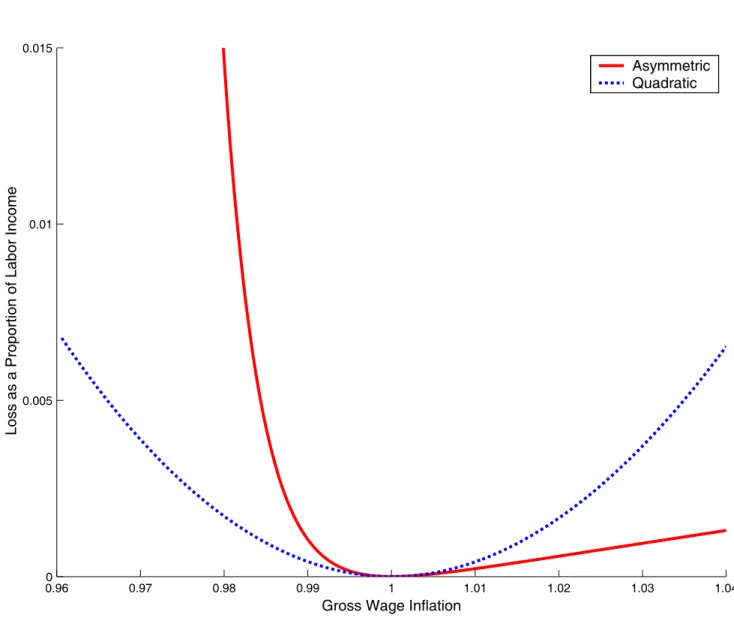
This section derives and evaluates the model predictions for higher-order moments of the variables. This exercise is important for three reasons. First, in contrast to linear DSGE models that inherit their higher-order properties directly from the shock innovations, the nonlinear propagation mechanism in our model means that economic variables may be non-Gaussian, even if the productivity innovations are Gaussian. Second, this observation means that up to the extent that actual data has non-Gaussian features, comparing the higher-order moments predicted by the model with those of the data may be a useful tool in model evaluation. Finally, since previous literature on downward wage rigidity documents the positive skewness of individual nominal wage changes, it is interesting to examine whether the same is true for the representative household in our model.

The skewness and kurtosis predicted by the models with asymmetric and quadratic wage adjustment costs are computed on the basis of 10000 simulated observations and reported in Table 2, along with their respective counterparts computed using U.S. data. In the U.S. data, the nominal interest rate and the rates of price and wage in ation are positively skewed and leptokurtic, consumption is negatively skewed and leptokurtic, and hours worked and the real wage are mildly skewed but platykurtic. (Leptokurtic distributions are characterized by a sharp peak at the mode and fat tails, while platykurtic distributions are characterized by atter peaks around the mode and thin tails.)

The model with quadratic wage adjustment costs generally predicts distributions with little or no skewness and kurtosis similar to that of the Normal distribution. In contrast, the model with asymmetric costs predicts positively skewed and leptokurtic rates of nominal interest, price in ation and wage in ation. The prediction of leptokurtic wage in ation is in agreement with microeconomic studies based on individual wage changes (see, among others, Akerlof, Dickens and Perry, 1996). Predictions regarding consumption are relatively more accurate than those of the quadratic model in that consumption is leptokurtic is negatively skewed, though in the latter case not as much as in the data. On the other hand, both

models deliver rather imperfect predictions regarding hours worked and the real wage. In particular, the asymmetric cost model predicts negatively skewed hours and thick-tailed distributions for hours and real wage than in the data. These results are summarized in Figure 4 that plots the histograms for price and wage in ation in the data and for both models.

4.4

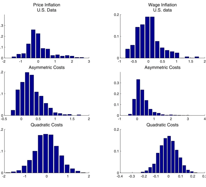
Comparison with Strict In ation Targeting

In order to better understand the degree of optimal grease in ation under the Ramsey policy, this section computes the in ation rate that delivers the highest (unconditional) welfare when the monetary authority follows a simple rule that strictly hits the in ation target. Figure 5 plots unconditional welfare for di erent values of the in ation target and indicates that, given the estimated parameters, the optimal in ation target would be around 3 percent per year. This value is more than twice as large as that of the Ramsey policy. The reason is that positive in ation in a model with downward wage rigidity is driven by prudence. With limited knowledge and less exibility with respect to shocks, the in ation targeting government needs a larger bu er above zero in ation to eschew paying the costs associated with nominal wage cuts.

5

Conclusion

This paper investigates Tobin's proposition that in ation greases the wheels of the labor market in the context of a simple but fully-speci ed dynamic general equilibrium model. Previous research based on linearized DSGE models did not examine this issue because, by construction, linearization eliminates the asymmetries of the underlying model. Although microeconomic research documents asymmetries in the raw wage data, the micro data itself contains elements of both economic structure and individual behavior and cannot fully reveal the mechanism through which downward wage rigidity may generate aggregate implications. Furthermore, the question is important because of the current discrepancy between theory| that prescribes zero-to-negative in ation rates|and actual practice|where central banks target low, but positive, in ation rates.

SMM estimates based on the second order approximation of model indicate that U.S. nominal wages are downwardly rigid, that optimal grease in ation is approximately 1.2 per-cent per year, and that downward wage rigidity has nontrivial implications for the dynamics of aggregate variables. Needless to say, the estimate of optimal grease in ation may depend on the model speci cation. For example, in a model with ex-post heterogeneity, optimal

grease in ation may be larger because productivity growth (and hence real wages) would vary across agents. In contrast, in a model with technological growth, optimal grease in a-tion may be smaller because a positive trend growth in real wages would decrease the need for nominal wage cuts. In ongoing and future work, we study these questions in the context of a fully- edged monetary economy, examine the role of asymmetric shocks, and derive the business cycle implications of asymmetric nominal rigidities.

Table 1. SMM Estimates

Wage Adjustment Costs Parameter Description Asymmetric Quadratic

(1) (2) Discount rate 0:998 0:998 (0:166) (0:402) Consumption curvature 1:093 0:874 (0:108) (0:222) Leisure curvature 3:6 10 6 _{1:2 10} 6 (0:418) (1:095) Wage adjustment cost 33:72y 71:98

(25:08) (136:4) Price adjustment cost 35:23 7:687

(20:08) (7:215)

Wage asymmetry 901:40 0

(426:2)

Autoregressive coe cient 0:927 0:922 (0:018) (0:027) Standard deviation 0:012 0:012

(0:002) (0:002)

Notes: The gures in parenthesis are standard errors. The superscripts and _{y denote the} rejection of the hypothesis that the true parameter value is zero at the 5 and 10 percent signi cance level, respectively.

Table 2. Higher-Order Moments

Wage Adjustment Costs Variable U.S. Data Asymmetric Quadratic

(1) (2) (3) A. Skewness Consumption 1:049 0:101 0:016 Hours 0:215 1:027 0:073 Price In ation 1:115 0:992 0:028 Wage In ation 0:821 1:655 0:083 Real Wage 0:233 0:081 0:039 Nominal Interest 1:030 0:576 0:155 B. Kurtosis Consumption 4:030 3:023 2:965 Hours 2:152 4:776 3:078 Price In ation 4:872 4:640 3:119 Wage In ation 4:515 7:826 3:153 Real Wage 1:820 2:916 2:937 Nominal Interest 4:333 3:679 3:153

Notes: The skewness and kurtosis predicted by the asymmetric and quadratic cost models were computed using 10000 simulated observations. The skewness and kurtosis of the Normal distribution are 0 and 3, respectively.

References

[1] Akerlof, G. A., W. T. Dickens, and G. L. Perry, (1996), \The Macroeconomics of Low In ation," Brookings Papers on Economic Activity, pp. 1-76.

[2] Bewley, T. F., (1995), \A Depressed Labor Market as Explained by Participants," American Economic Review 85, pp. 250-254

[3] Billi, R., (2005), \The Optimal In ation Bu er with a Zero Bound on Nominal Interest Rates," Center for Financial Studies Working Paper No. 2005/17.

[4] Card, D. and D. Hyslop, (1997), \Does In ation Greases the Wheels of the Labor Market?" in Reducing In ation: Motivation and Strategy, C. Romer and D. Romer, eds., Chicago: University of Chicago Press.

[5] Campbell, C. M. and K. S. Kamlani, (1997), \The Reasons for Wage Rigidity: Evidence from a Survey of Firms," Quarterly Journal of Economics 112, pp. 759-790.

[6] Castellanos, S. G., R. Garcia-Verdu, and D. S. Kaplan, (2004), \Nominal Wage Rigidity in Mexico: Evidence from Social Security Records," Journal of Development Economics 75, pp. 507-533.

[7] Chari, V. V. and P. J. Kehoe, (1999), \Optimal Fiscal and Monetary Policy," in Hand-book of Macroeconomics, J. B. Taylor and M. Woodford, eds., pp. 1671-1745, Amster-dam: Elsevier.

[8] Christiano, L. J., M. Eichenbaum, and C. L. Evans, (2005), \Nominal Rigidities and the Dynamic E ects of a Shock to Monetary Policy," Journal of Political Economy 113, pp. 1-45.

[9] Du e, D. and Singleton, K. J., (1993), \Simulated Moments Estimation of Markov Models of Asset Prices," Econometrica 61, pp. 929-952.

[10] Fehr, E. and L. Goette, (2005), \Robustness and Real Consequences of Nominal Wage Rigidity," Journal of Monetary Economics 52, pp. 779-804.

[11] Friedman, M., (1969), The Optimum Quantity of Money and Other Essays, Chicago: Aldine.

[12] Hansen, G. D., (1985), \Indivisible Labor and the Business Cycle," Journal of Monetary Economics 16, pp. 309-327.

[13] Ireland, P., (2001), \Sticky-Price Models of the Business Cycle: Speci cation and Sta-bility," Journal of Monetary Economics 47, pp. 3-18.

[14] Jin, H. and K. L. Judd, (2002), \Perturbation Methods for General Dynamic Stochastic Models," Hoover Institution, Mimeo.

[15] Gallant, A. R., P. E. Rossi, and G. Tauchen, (1993), \Nonlinear Dynamic Structures," Econometrica 61, pp. 871-908.

[16] Kahneman, D., J. L. Knetsch, and R. Thaler, (1986), \Fairness as a Constraint on Pro t Seeking: Entitlements in the Market," American Economic Review 76, pp. 728-41. [17] Keynes, J. M., (1936), The General Theory of Employment, Interest and Money,

Cam-bridge: Macmillan Cambridge University Press.

[18] Khan, A., R. G. King and A. Wolman, (2003), \Optimal Monetary Policy," Review of Economic Studies 70, pp. 825-860.

[19] Kim, J., (2000), \Constructing and Estimating a Realistic Optimizing Model of Mone-tary Policy," Journal of MoneMone-tary Economics 45, 329-359.

[20] Kim. J., S. Kim, E. Schaumburg and C. Sims, (2003), \Calculating and Using Second-Order Accurate Solutions of Discrete Time Dynamic Equilibrium Models," Finance and Economics Discussion Series No. 2003-61, Federal Reserve Board.

[21] Kim, J. and D. W. Henderson, (2005), \In ation Targeting and Nominal Income Growth Targeting: When and Why are They Suboptimal?" Journal of Monetary Economics 52, pp. 1463-1496.

[22] Koop, G., M. H. Pesaran, and S. Potter, (1996), \Impulse Response Analysis in Non-linear Multivariate Models," Journal of Econometrics 74, pp. 119-147.

[23] Kuroda, S. and I. Yamamoto, (2003), \Are Japanese Nominal Wages Downwardly Rigid? (Part I): Examination of Nominal Wage Change Distributions," Monetary and Economic Studies 21 (August), pp. 1-30.

[24] Lee, B.-S. and Ingram, B. F., (1991), \Simulation Estimation of Time-Series Models," Journal of Econometrics 47, pp. 195-205.

[25] McLaughlin, K. J., (1994), \Rigid Wages?" Journal of Monetary Economics 34, pp. 383-414.

[26] Peltzman, S., (2000), \Prices Rise Faster than They Fall," Journal of Political Economy 108, pp. 466-502.

[27] Rotemberg, J. J., (1982), \Sticky Prices in the United States," Journal of Political Economy 90, pp. 1187-1211.

[28] Rotemberg, J. J. and M. Woodford, (1997), \An Optimization-Based Econometric Model for the Evaluation of Monetary Policy," NBER Macroeconomics Annual 12, pp. 297-346.

[29] Ruge-Murcia, F. J., (2007), \Methods to Estimate Dynamic Stochastic General Equi-librium Models," Journal of Economic Dynamics and Control 31, pp. 1599-2636. [30] Schmitt-Grohe, S. and M. Uribe, (2004), \Optimal Fiscal and Monetary Policy Under

Sticky Prices," Journal of Economic Theory 114, pp. 198-230.

[31] Schmitt-Grohe, S. and M. Uribe, (2004), \Solving Dynamic General Equilibrium Models Using a Second-Order Approximation to the Policy Function," Journal of Economic Dynamics and Control 28, pp. 755-775.

[32] Schmitt-Grohe, S. and M. Uribe, (2006), \Optimal In ation Stabilization in a Medium-Scale Macroeconomic Model," in Gertler, M. and K. Rogo , eds. NBER Macroeconomics Annual, MIT Press: Cambridge MA, pp. 383{425.

[33] Teles, P., (2003), \The Optimal Price of Money," Federal Reserve Bank of Chicago Economic Perspective, 29:1, pp. 29{39.

[34] Tobin, J., (1972), \In ation and Unemployment," American Economic Review 62, pp. 1-18.

[35] Varian, H., (1974), \A Bayesian Approach to Real Estate Assessment," in Studies in Bayesian Economics in Honour of L. J. Savage, S. E. Feinberg and A Zellner, eds., Amsterdam: North-Holland.

[36] Zbaracki, M., M. Ritson, D. Levy, S. Dutta, and M. Bergen, (2004), \Managerial and Customer Costs of Price Adjustment: Direct Evidence from Industrial Markets," Review of Economics and Statistics 86, pp. 514-533.

0.96 0.97 0.98 0.99 1 1.01 1.02 1.03 1.04 0

0.005 0.01 0.015

Gross Wage Inflation

Loss as a Proportion of Labor Income

Asymmetric Quadratic

2 4 6 8 10 12 14 -4 -2 0 2 4 Consumption 2 4 6 8 10 12 14 -2 -1 0 1 2 Hours 2 4 6 8 10 12 14 -1 -0.5 0 0.5 1 Price Inflation 2 4 6 8 10 12 14 -0.2 -0.1 0 0.1 0.2 Wage Inflation 2 4 6 8 10 12 14 -2 -1 0 1 2 Real Wage 2 4 6 8 10 12 14 -1 -0.5 0 0.5 1 Nominal Interest +2σ +1σ -1σ -2σ ss

Figure 2: Responses to a Productivity Shock

Quadratic Wage Adjustment Costs

2 4 6 8 10 12 14 -4 -2 0 2 4 Consumption +2σ +1σ -1σ -2σ ss 2 4 6 8 10 12 14 -2 -1 0 1 2 Hours 2 4 6 8 10 12 14 0 0.5 1 Price Inflation 2 4 6 8 10 12 14 0 0.5 1 Wage Inflation 2 4 6 8 10 12 14 -2 -1 0 1 2 Real Wage 2 4 6 8 10 12 14 -0.2 0 0.2 0.4 0.6 0.8 Nominal Interest

Figure 3: Responses to a Productivity Shock

Asymmetric Wage Adjustment Costs

-2 -1 0 1 2 3 0 0.1 0.2 0.3 Price Inflation U.S. Data -1 -0.5 0 0.5 1 1.5 2 0 0.1 0.2 Wage Inflation U.S. data -0.50 0 0.5 1 1.5 2 0.1 0.2 Asymmetric Costs -1 0 1 2 3 4 0 0.1 0.2 0.3 Asymmetric Costs -2 -1 0 1 2 0 0.1 0.2 Quadratic Costs -0.40 -0.3 -0.2 -0.1 0 0.1 0.2 0.3 0.1 0.2 Quadratic Costs

-7367.2 -7367.1 -7367.0 -7366.9 -7366.8 -7366.7 -7366.6 U n condi ti onal W e lf ar e 1 1.01 1.02 1.03 1.04 Inflation Target