Optical and mechanical analysis on a biological cell in optical tweezers

Optical and mechanical analysis on a biological cell in

optical tweezers

Thèse

Lingyao Yu

Doctorat en physique

Philosophiae doctor(Ph.D.)

Québec, Canada

© Lingyao Yu, 2016

Optical and mechanical analysis on a biological cell in

optical tweezers

Thèse

Lingyao Yu

Sous la direction de :

Yunlong Sheng

Résumé

La réponse mécanique d'une cellule à une force externe permet d'inférer sa structure et fonction. Les pinces optiques s'avèrent une approche particulièrement attrayante pour la manipulation et caractérisation biophysique sophistiquée des cellules de façon non invasive. Cette thèse explore l’utilisation de trois types de pinces optiques couramment utilisées : 1) statiques (static), 2) à exposition partagée (time-sharing) et 3) oscillantes (oscillating). L’utilisation d’un code basé sur la méthode des éléments finis en trois dimensions (3DFEM) nous permet de modéliser ces trois types de piégeage optique afin d’extraire les propriétés mécaniques cellulaires à partir des expériences.

La combinaison des pinces optiques avec la mécanique des cellules requiert des compétences interdisciplinaires. Une revue des approches expérimentales sur le piégeage optique et les tests unicellulaires est présentée. Les bases théoriques liant l’interaction entre la force radiative optique et la réponse mécanique de la cellule aussi. Pour la première fois, une simulation adaptée (3DFEM) incluant la diffusion lumineuse et la distribution du stress radiatif permet de prédire la déformation d’une cellule biconcave –analogue aux globules rouges—dans un piège statique double (static dual-trap). À l’équilibre, on observe que la déformation finale est donnée par l’espacement entre les deux faisceaux lasers: la cellule peut être étirée ou même comprimée.

L’exposition partagée (time-sharing) est la technique qui permet de maintenir plusieurs sites de piégeage simultanément à partir du même faisceau laser. Notre analyse quantitative montre que, même oscillantes, la force optique et la déformation sont omniprésentes dans la cellule : la déformation viscoélastique et la dissipation de l’énergie sont analysées. Une autre cellule-type, la tige cubique, est étudiée : cela nous permet d’élucider de nouvelles propriétés sur la symétrie de la réponse mécanique.

Enfin, l’analyse de la déformation résolue en temps dans un piége statique ou à exposition partagée montre que la déformation dépend simultanément de la viscoélasticité, la force externe et sa forme tridimensionnelle. La technique à force oscillante (oscillating tweezers) montre toutefois un décalage temporel, entre la force et la déformation, indépendant de la forme 3D; cette approche donnerait directement accès au tenseur viscoélastique complexe de la cellule.

Abstract

The mechanical response of a cell to external forces carries information about its structure and function. Because cell manipulation should ideally be non-invasive while performing sophisticated biophysical characterization, the radiation force of optical tweezers has become highly attractive. In this thesis, we explore three types of recently-developed optical tweezers: 1) static, 2) time-sharing and 3) oscillating. Using a full three-dimensional finite element method (3DFEM), modeling of each of these regimes allows us to fit experiments and access the cell mechanical properties.

Combining optical trapping with cell mechanics requires interdisciplinary efforts. A survey of the various experimental approaches for optical trapping and measurements on isolated cells is presented. We then lay the theoretical background linking the interaction of optical fields to the cell’s mechanical response. We are the first to implement a 3DFEM calculation including light scattering and the radiation stress distribution to predict the deformation of a biconcave cell –emulating a red blood cell– in static dual-trap optical tweezers. At equilibrium, the final deformation is given by the separation distance of the two trapping beams, revealing how the cell can be elongated or shrunk.

Time-sharing optical tweezers realize multiple traps to manipulate objects ranging from macromolecules to biological cells. Our quantitative analysis shows how, although jumping, the local stress and strain is omnipresent in the cell. The viscoelastic object deformation and internal energy dissipation are analyzed. Another cell shape, a cubic rod, is also studied, elucidating novel symmetrical properties of the mechanical response.

Finally, the analysis of the time-dependent deformation –creep testing– of a cell in static and time-sharing optical tweezers, shows that deformation of the object depends altogether on the object’s viscoelasticity, significantly on its 3D shape and the mechanical loading. However,

dynamic testing with oscillating optical tweezers surprisingly shows a phase shift between the loading stress (external force) and strain (deformation) independent on the 3D cell shape. This is a novel avenue giving access to the cell’s viscoelasticity dynamic complex modulus directly in the time-domain.

Content

Résumé ... III Abstract ... V Content ... VII List of tables ... IX List of figures ... X Abbreviations ... XII Acknowledgement ... XIV Foreword ... XVI 1. Introduction ... 1

1.1. Cell mechanics and its testing ... 1

1.2. Manipulation by optical tweezers ... 4

1.2.1. Measurement in equilibrium state ... 4

1.2.2. Creep testing ... 7

1.2.3. Dynamic testing ... 11

1.3. Theoretical analysis of electromagnetic field ... 15

1.3.1. Electromagnetic field of trapping beams ... 16

1.3.2. Optical radiation force ... 19

1.4. Modeling methods quantifying mechanical properties of cells ... 20

1.4.1. 1D viscoelastic model ... 21

1.4.1.1. Spring-dashpot model ... 23

1.4.1.2. Power-law model ... 27

1.4.2. 3D multi-layer model ... 29

1.4.2.1. Hyperelastic membrane & viscous cytosol ... 30

1.4.2.2. Hyperelastic and viscoelastic membrane & viscous cytosol ... 33

1.4.2.3. Viscoelastic bilayer & hyperelastic cytoskeleton & fluid cytosol ... 36

1.5. Research subjects, objective and organization of the thesis ... 38

1.5.1. Research subjects ... 38

1.5.2. Objectives & organization ... 40

1.6. References ... 41

2. Three-dimensional light-scattering and deformation of individual biconcave human blood cells in optical tweezers ... 48

2.1. Résumé ... 48

2.2. Abstract ... 49

2.3. Introduction ... 49

2.4. Scattering of the RBC in dual-trap tweezers ... 51

2.5. Maxwell stress tensor ... 56

2.7. Results ... 62

2.8. Conclusion ... 64

2.9. Acknowledgments ... 65

2.10. References ... 65

3. Mechanical analysis of the optical tweezers in time-sharing regime ... 67

3.1. Résumé ... 67

3.2. Abstract ... 68

3.3. Introduction ... 68

3.4. Temporal response of a viscoelastic 1D rod ... 69

3.5. Spatial response of 3D object ... 76

3.6. Conclusion ... 79

3.7. Appendix ... 80

3.8. Acknowledgments ... 81

3.9. References ... 81

4. Temporal response of 3D biological cell to high-frequency optical jumping tweezers 83 4.1. Résumé ... 83

4.2. Abstract ... 84

4.3. Introduction ... 84

4.4. Temporal Mechanical Response ... 85

4.4.1. 1D Spring and Dashpot Model ... 85

4.4.2. 1D Response in x-direction ... 86

4.4.3. Displacements in y- and z-directions... 90

4.5. Compare Deformations of Two Objects ... 92

4.6. Conclusion ... 96

4.7. References ... 96

5. Effect of the object 3D shape on the viscoelastic testing in optical tweezers ... 98

5.1. Résumé ... 98

5.2. Abstract ... 99

5.3. Introduction ... 99

5.4. Creep response to step load ... 101

5.5. Dynamic response to sinusoidal load ... 107

5.6. Conclusion ... 113

5.7. Appendix ... 114

5.8. References ... 115

6. Conclusions and perspectives ... 118

6.1. Conclusions ... 118

6.2. Perspectives ... 120

6.3. References ... 122

List of tables

Table 4.1 Comparison of the deformations of two objects of different 3D shapes in the jumping optical tweezers. ... 95 Table 5.1 Characteristic creep testing for three solid body objects. ... 105 Table 5.2 Characteristic creep testing for three objects of viscoelastic membrane. ... 107

List of figures

Figure 1.1 Schematic of experimental techniques of the cell manipulations ... 3

Figure 1.2 Single cell manipulation with microbeads adhered to cell by optical tweezers .... 5

Figure 1.3 Single cell manipulation without microbeads by dual-trap optical tweezers ... 6

Figure 1.4 Time-sharing optical setup controlled by AOM ... 8

Figure 1.5 Cell deformations in optical jumping tweezers ... 9

Figure 1.6 Optical stretcher setup and measurements of creep ... 10

Figure 1.7 Optical trapping system for dynamic testing and loss tangent measurements .... 12

Figure 1.8 Dynamic testing of the high-throughput flow cytometry ... 14

Figure 1.9 Cellular mechanical responses to the dynamic testing ... 14

Figure 1.10 Scheme of the radial polarization of the spherical wavefront ... 19

Figure 1.11 stress-strain behaviors of viscoelastic testing methods ... 23

Figure 1.12 Schematic diagrams of spring-dashpot models ... 24

Figure 1.13 Schematic of SLS model ... 25

Figure 1.14 Time-dependent mechanical modulus... 29

Figure 1.15 Cell membrane constructions and its mechanical material model ... 30

Figure 1.16 Cell deformations in experiments and simulations ... 32

Figure 1.17 Curves of the relaxation time in the process of cell recovery ... 34

Figure 1.18 Fluid-structure interaction model and the simulation results ... 36

Figure 1.19 Multilayer model of red blood cell and table of simulation results ... 38

Figure 2.1 Geometrical illustration of RBC in optical tweezers ... 54

Figure 2.2 Electromagnetic field distribution on the surface of RBC ... 55

Figure 2.3 Electromagnetic field distribution in the internal cross sections of RBC ... 56

Figure 2.4 Optical radiation stress distributions ... 59

Figure 2.5 flow chart of two-way coupled computation ... 62

Figure 2.6 3D deformation of an RBC in dual-trap tweezers. ... 64

Figure 3.1 Stress distribution along a 1D rod under the right-hand side loading ... 71

Figure 3.2 Scheme of SLS model. ... 72

Figure 3.3 Time-dependent stress and strain curves ... 74

Figure 3.4 Rod elongation in jumping loadings ... 74

Figure 3.5 Stress-strain curve of the hysteresis loop ... 75

Figure 3.6 Stress and strain distribution in the cross section of the cell disk ... 78

Figure 3.7 Principal stress distribution in the cross section of a deformed RBC ... 79

Figure 4.1 Viscoelastic standard linear solid (SLS) material model ... 86

Figure 4.2 Viscoelastic cubic rod with landmark spots ... 87

Figure 4.3 Time-dependent curves of the local stress and strain ... 88

Figure 4.4 Creep behavior of the rod in jumping loadings ... 89

Figure 4.6 Strain tensor components of local points ... 92

Figure 4.7 Scheme of a quarter of the biconcave object and a quarter of the cubic rod. ... 94

Figure 4.8 Elongation of the biconcave object and the cubic rod in x-direction. ... 95

Figure 5.1 Geometric models of the viscoelastic material ... 103

Figure 5.2 Creep behaviors of three 3D objects and 1D SLS model... 104

Figure 5.3 3D distribution of local stress σxx component in three solid body objects ... 105

Figure 5.4 Stress distribution in the membrane ... 106

Figure 5.5 Stress and strain behavior in dynamic testing ... 112

Abbreviations

AFM atomic force microscopy MTC magnetic twisting cytometry pN pico-newton

RBC red blood cell BE beam expander

PBS polarizing beam splitter HW half-wave

NEM N-ethylmaleimide

MS motorized translational stage Neu neutrophil

Mono monocyte Mac Macrophages HL60 undifferentiated cell FEM finite element method 1D one-dimension

3D three-dimension

AOM acousto-optic modulator AOD acousto-optic deflector FDTD finite-difference time-domain NA numerical aperture

QPD quadrant photodiode CCD charge-coupled device SLS standard linear solid RF radio frequency

FSI fluid-structure interaction cw continuous wave

Acknowledgement

First of all, I am sincerely grateful to my supervisor, Prof. Yunlong Sheng, who provided me with the great opportunity to come to Canada to pursue my PhD studies at the Laval University. Since my first arrival to Quebec City from China, Prof. Sheng helped me a lot to adapt to both living and studying. Because of his continuous help, scientific advice, professional guidance and constant encouragement, I could overcome every challenge I met to finish my PhD project during my study.

What’s more, I would like to thank Prof. Arthor Chiou who is from the Institute of Biophotonics & Biophotonics Interdisciplinary Research Center (BIRC), National Yang-Ming University, Taipei, Taiwan, for providing us with precious experimental results and experiences.

I would also like to thank Prof. Simon Rainville, Prof. Simon Thibeault and Prof. Daniel Coté. Thank you for your kind instructions in your courses and I have learned different learning methods in experiment from I experienced in China.

I express my sincere gratitude to Mr. Martin Blouin for his kindness and prompt technical assistances. I also want to thank my colleague Dr. Francois Bordeleau who helped me know more about our optical tweezers system. At the same time, I would also like to express my deep gratitude to my colleagues Dr. Samir Sahli, Dr. Guilleum Tremblay, Dr. Michel Auclair, Yann Gravel, Dr. Paul Brule-Bareil, Jing Wang, Yuhua Yang and Dr. Kejia Wang for your helpful discussions and advices in our enjoyable working environment.

I want to thank Prof. Julien Beaudoin Bertrand who is my mentor during my research assistant work since January 2015. Thanks for your careful corrections of my thesis abstract and resumé.

I also acknowledge jury members, Prof. Yunlong Sheng, Prof. Simon Rainville, Prof. Tigran Galstian from COPL in Laval University and Prof. H. Daniel Ou-Yang from Lehigh University, US as well as our program director, Prof. Laurent Drissen. I read your comments carefully and they are very valuable for me. For your kind understanding and support I can have my phD defense in videoconference early in the morning while Prof. Ou-Yang is in Japan at mid-night.

I appreciate all the staff in COPL (Center for Optics, Photonics and Lasers) who are always kind and ready to help me with any requirement. I am also thankful to the stuff from Compute Canada for their technical support in HPC (high performance computing) for my simulation work.

Finally, I would like to express my greatest thanks to my family. Thank you, my parents. I can face up and deal with any difficulty in my life for your endless love and encouragement. And thank you, my husband. Although we are oceans away, I know your support for me is every moment.

Thank you for all

Foreword

Four published papers are inserted into the thesis from chapter 2 to chapter 5, respectively. I am the first author of these papers.

1. Lingyao Yu, Yunlong Sheng, and Arthur Chiou, Three-dimensional light-scattering and deformation of individual biconcave human blood cells in optical tweezers, Optics Express Vol. 21, Iss. 10, pp. 12174–12184 (2013). This paper was selected to publish in Virtual Journal for Biomedical Optics (VJBO) Vol. 8, Iss. 6, (2013) (Optical Traps, Manipulation, and Tracking).

In this paper, I conducted the 3D modeling and simulation work in FEM. Prof. Sheng contributed the idea. Prof. Chiou provided the experimental details. Both Prof. Sheng and I wrote the paper. Multiply revisions were done by Prof. Sheng.

2. Lingyao Yu and Yunlong Sheng, Mechanical analysis of the optical tweezers in time-sharing regime, Optics Express Vol. 22, Iss. 7, pp. 7953–7961 (2014). This paper was selected to publish in Virtual Journal for Biomedical Optics (VJBO) Vol. 9, Iss. 6, (2014) (Optical Traps, Manipulation, and Tracking).

In this paper, I implemented the 3D modeling and simulation work in FEM. Prof. Sheng contributed the idea. Both Prof. Sheng and I wrote the paper. I discussed a lot with Prof. Sheng. Multiply revisions were done by Prof. Sheng.

3. Lingyao Yu and Yunlong Sheng, Temporal response of three-dimensional biological cells to high-frequency optical jumping tweezers, Journal of Nanophotonics,Vol. 9, 093083 (2015).

In this paper, I conducted the 3D modeling and simulation work in FEM. Both Prof. Sheng and I contributed the idea. Both Prof. Sheng and I wrote the paper. Multiply revisions were done by Prof. Sheng.

4. Lingyao Yu and Yunlong Sheng, Effect of the object 3D shape on the viscoelastic testing in optical tweezers, Optics Express, Vol. 23, Iss. 5, pp. 6020-6028, (2015). This paper was also published in virtual journal of Optics Express Joint Feature Issue with Optics Express and Journal of the Optical Society of America B: Optical Cooling and Trapping (2015); JOSA B Joint Feature Issue with Journal of the Optical Society of America and Optics Express: Optical Cooling and Trapping (2014). This paper was selected to publish in Virtual Journal for Biomedical Optics (VJBO) Vol. 10, Iss. 4, (2015) (Optical Traps, Manipulation, and Tracking).

In this paper, I did the most scientific work like contributing the idea, the 3D modeling and simulation work in FEM. Both Prof. Sheng and I wrote the paper. I discussed a lot with Prof. Sheng. Multiply revisions were done by Prof. Sheng.

Co-authors:

Yunlong Sheng: Center of Optics, Photonics and Laser, Department of Physics,

Engineering Physics and Optics, Laval University. 2375 rue de la Terrasse Quebec, Quebec G1V 0A6.

Author Chiou: Institute of Biophotonics, Biophotonics and Molecular Imaging Research

Center (BMIRC) National Yang-Ming University, No. 155, Sec. 2, Linong Street, Taipei 11221, Taiwan.

1.

Introduction

1.1.

Cell mechanics and its testing

As a basic unit of life, the biological cell is a complicated system. Cells can grow, reproduce, process information, respond to stimuli, and carry out an amazing array of chemical reactions. Cells could also control and respond to a great number of intra and extracellular events. During the past centuries, studies on cell activities draw from diverse fields, including biology, physiology, biophysics, and biochemistry. As a part of cells activities, the cell mechanics, referring to the motion and deformation of the cells and the interaction between the cells, is about how the cells sense mechanical forces, transmit them into the cell and convert the mechanical forces into biochemical responses [1]. With this mechanotransduction ability, a variety of biological pathways in the cell will occur and result in diverse effects such as alterations in membrane channel activity, transmission of signals, regulations of gene expression, changes in protein synthesis, deformation of the cell morphology, etc. [2]. For example, as the diameter of the erythrocytes (red blood cell, RBC) is often larger than that of small capillaries through which cells must pass to transport O2 or CO2 molecules in the normal microcirculation, an RBC needs to change its normal biconcave shape to a bullet or parachute shape because the RBC is larger than the capillary diameter. Some biological changes in the cells are associated with a wide spectrum of pathologies. The mechanical properties of RBCs could be converted by the protozoan Plasmodium falciparum, the single-cell parasites which cause the extensive molecular and structural changes stiffening the cell membranes and result in malaria [3]. Additional pathologies, such as cancer metastasis [4], atherosclerosis [5], asthma [6], pharmacological traitements [7] and sickle cell diseases [8], are all strongly related to the cellular mechanical properties. Thus, the mechanisms by which cells respond to external forces and the connection between cell mechanics and function could be significant to the

investigation of human diseases.

In the last few decades a number of experimental methods for probing the cellular stiffness have been proposed and improved. The cellular deformation can be observed and measured by using the optical microscopy with high precision [2]. Figure 1.1 illustrates commonly used testing methods of the single cell manipulation, (a): atomic force microscopy (AFM) [9-11], (b): microindentation or cell poking [12], (c): shear flow [13], (d): micropipette aspiration [14, 15], (e): cell plated on micropillars which deform under the cellular traction force [16], (f): substrate strain [17, 18], (g): magnetic twisting cytometry (MTC) [19, 20], (h): optical tweezers with microbeads contact [21, 22], (i): optical stretcher [23, 24], and (j): optical tweezers without beads contact [25, 26]. In these techniques, the loading forces applied on the cell can be concentrated forces (e.g. AFM), distributed forces (e.g. microplate manipulation), transient forces (e.g. micropipette aspiration) or dynamic loading (e.g. oscillatory MTC or time-sharing optical tweezers). The forces can be either indirectly (e.g. optical tweezers or MTC with beads) or directly applied to the cells (e.g. optical tweezers without beads contact or optical stretcher). Different types of experimental techniques testing the mechanical properties lead to a variety of mechanical models that are used to quantify the cell mechanical responses. For example, the instantaneous modulus of human chondrocytes by using the AFM is 290 ± 140 Pa, but the same parameter measured by cytoindentation is 630 ± 510 Pa [27, 28]. In addition, there has been no universal mechanical model available in any physiological and microenvironmental condition to assess the adaptive behavior of the living cells which dynamically adapt to their surroundings [29]. Therefore, one can choose the feasible modeling, define material properties and calculate the force- deformation behaviors of the cells with respect to a certain experimental technique to help further understand the complex cellular structure-function interactions and material properties of cells. In this paper, we focus on the cell manipulation with the optical tweezers.

Figure 1.1Schematic of experimental techniques of the cell manipulations

(a): Atomic force microscopy (AFM); (b): microindentation or cell poking; (c): fluid shear flow; (d): micropipette aspiration; (e): cell lying on a bed of microneedles that deform under cellular traction force; (f): substrate strain experiments; (g) magnetic twisting cytometry; (h): optical tweezers with microbeads contact; (i): optical stretcher; (j): optical tweezers without beads contact (the trapping beams could be static or vibrated at a certain frequency).

1.2.

Manipulation by optical tweezers

When a laser beam is incident to an object, whose refractive index is difference from that of the surrounding buffer, the optical refraction and reflection occur, that results in optical radiation force following the law of the conservation of momentum. The radiation force is in the pico-Newton (pNs) range, which is in the same order of magnitude of the forces within and between the biological cells. Thus, the laser beam can be used to trap and manipulate the object at sub-nanometer (nm) resolutions. Optical tweezers have been widely used to manipulate the single biological cell and to probe its mechanical properties with or without the beads contact [26, 30-33]. In the optical tweezers, the laser beam is highly focused into the dielectric object (microbeads or the biological cell) by using the oil or water immersion objective with high numerical aperture (NA). The trapping laser beam at the wavelength of 1064 nm is commonly used because the absorption of the biological cells or tissues in the spectral range from about 700 to 1100 nm is minimum [34]. Cells can be also trapped and stretched directly by two non-focused counter-propagating laser beams in an optical stretcher or screened by the laser traps when cells pass through the flow cytometry[23, 35]. In the test of mechanical properties of the cell, the manipulation of the cell by the optical tweezers can be with or without microbeads adhered to the cell. The trapping beams could be static, time-sharing, and oscillating. Some typical trapping methods are introduced in this subsection.

1.2.1.

Measurement in equilibrium state

In order to measure the elastic properties of the cell membrane, the commonly used method is to measure the final deformation of the trapped cell at the equilibrium state. The optical trapping forces could achieve up to hundreds of pN. In the numerical analysis, the elasticity

of the cell can be calculated based on the linear elastic or hyperelastic material models.

Cell manipulation with microbeads is to trap and move coated microbeads of the higher

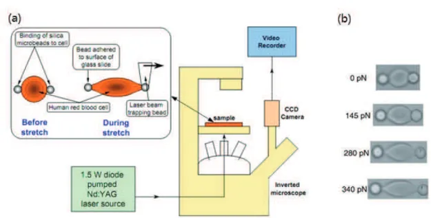
refractive index than the buffer solution with the beads adhered to the cell surface. When two microbeads are attached to diametric ending sides of a cell, one microbead is adhered to the surface of the glass slide while the other is trapped and moved by the optical tweezers, large deformation of the cell could be realized. In this approach the optical trapping forces can be large, resulting in large deformation of the cell.[21, 36]. The optical setup is shown in Fig. 1.2(a) [21]. The 1.5 W Nd:YAG laser beam is sent into the objective of an inverted microscope. The CCD camera and video recorder record the whole process of the cell deformation in axial and transverse directions. The optical forces are different by varying the laser power. The final deformations of the cell at equilibrium state are recorded with different loading forces from 0 to 340 pN, as shown in Fig. 1.2(b) [21].

Figure 1.2 Single cell manipulation with microbeads adhered to cell by optical tweezers

Scheme of optical tweezers setup (a); Images of deformed cell loaded from 0 to 340 pN (b) [21].

Cell manipulation without microbeads: The trapping laser beams directly manipulate the

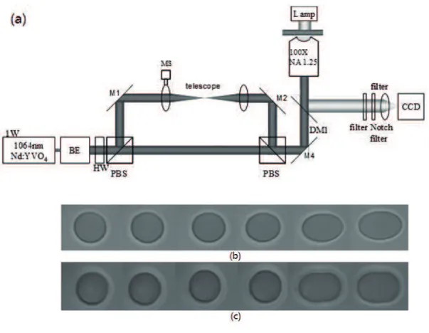
such non-invading manipulations. The dual-trap optical tweezers setup is illustrated in Fig. 1.3(a) [37]. A laser beam (1W, Nd: YVO4 cw laser) passes through a beam expander (BE) to overfill the back aperture of an oil immersion microscope objective (NA=1.25, 100X). The laser beam is split into two parallel trapping beams via a polarizing beam splitter (PBS) and recombined by a second PBS, focused in the focal plane of the objective lens;

Figure 1.3 Single cell manipulation without microbeads by dual-trap optical tweezers

Setup of a dual-trap optical tweezers for direct manipulating a cell (a). Images of a trapped and stretched red blood cell: without drug treatment (b) and with 1mM N-ethylmaleimide (NEM) treatment (c), for 30 minutes as a function of the dual beam separation: 0, 1.27, 2.54, 3.80, 5.07 and 6.34 µm, respectively (from left to right) [37].

the optical powers of the two beams can be adjusted by rotating the half-wave (HW) plate. One of the laser beams passes through a telescopic system consisting of two lenses. The

first lens is mounted on a motorized translational stage (MS) for displacing the beam in the direction transversal to the optical axis. This leads to a lateral shift of the focal spot of the trapping beam, without the beam walk-off at the entrance pupil of the objective lens. Wide-field images of the trapped and stretched cell are captured by a CCD camera for observation and analysis. The erythrocyte sample is suspended in the buffer solution and swollen to the spherical shape under osmosis pressure. The dual-trap beams are highly focused and side incident into the cell with a certain distance of beam separation. Figure 1.3(b) and 1.3(c) show the micrographic images for the cells of the final elongations without drug treatment and with 1mM N-ethylmaleimide (NEM) treatment for 30 minutes as a function of the dual-beam separation. The cell membrane’s elasticity coefficients are obtained by fitting to the experimental data with theoretical predictions. The red blood cells treated by NEM show different deformations from the normal cells [37].

1.2.2.

Creep testing

Instead of measuring the final elongation of the cell in the equilibrium state, the time- dependent mechanical response is also of interest for testing the cell’s viscoelastic properties [38, 39]. Creep testing is a commonly used method. When external loading forces are suddenly applied and kept constant, the object’s elongation may have an instantaneous jump followed by a slower increase to the final deformation at equilibrium state. The static optical tweezers with or without microbeads contact to the cell could be used in the creep testing.

Time-sharing optical tweezers using one laser beam to scan at different locations in the

cell at a high frequency, to mimic the multiple optical traps was proposed in 1993 [40]. In the experiment, the rapidly ‘blinking’ trap is approximated as the steady trap when the beam scans at a high frequency. The time-sharing technique can flexibly manipulate a

viscoelastic object among a set of positions in the specimen [41]. For example, one continuous wave (cw) laser beam (λ = 1064 nm) is sent into an acousto-optic modulator (AOM) at the Bragg angle; the zero order transmitted beam is blocked and the first order diffracted beam is directed to the two-lens telescopic system. The exit aperture of the AOM is imaged onto the entrance aperture of a microscope objective lens (NA=1.25) such that the angular scanning of the beam by the AOM is transformed into a lateral displacement of the focal spot without any beam walk-off at the entrance aperture, as shown in Fig. 1.4 [42]. The diffraction angle of the output beam is controlled by applying different radio-frequency (RF, 30-50 MHz) signals to the AOM. Both frequency and intensity of the acoustic signal can be changed rapidly by changing the modulation voltages. At the high jumping frequency of 1 kHz, the object is trapped and deformed, with no observable object vibration by naked eyes in the experiment. The cell’s elongations in the loading force axis are determined by the dual-trap beam separation. Both creep and recovery behaviors of the cell along the loading force axis are recorded as a function of the jumping distances (between 3.8 µm and 5.9 µm) [37, 42], as shown in Fig. 1.5. The mechanical properties of the cell could be obtained by choosing a theoretical model to fit the experimental data. The theoretical models for mechanical responses and material properties of the cell are introduced in the Subsection 1.3.

Figure 1.4 Time-sharing optical setup controlled by AOM

Figure 1.5 Cell deformations in optical jumping tweezers

Cell manipulation at different jumping distance (a); time-dependent elongation of cell at different jumping distances (b) [32].

In the Optical stretcher two slightly divergent counter-propagating laser beams are used to trap and stretch the single cell centered between the two single-mode optical fibers. The radii of the divergent laser beams (about 10 µm) in the plane of the trapped cell should be larger than the cell size [23, 43, 44]. Figure 1.6(a) shows the schematic of the microfluidic optical stretcher [24]. The light source at a wavelength of 785 nm is split into two beams which are coupled into two single-mode optical fibers by the fiber couplers after passing through the AOM. The images of the sample is collected by the objective and captured by a CCD camera. Two optical fibers should be strictly aligned such that the cell centered between the fibers could be trapped and stretched without any movement. As the radiation forces of the beams from two fibers on the cell must be equal to each other to keep the cell trapped, the biological cell is usually swollen to the spherical shape before being sent into the microfluidic optical stretcher. For example, Ekpenyong et al measured the different creep behaviors of three spherical lineages of human myeloid precursor cells, neutrophils (Neu), monocytes (Mono) and macrophages (Mac) as well as undifferentiated spherical cells (HL60) with the same optical system and physical conditions, as shown in Fig. 1.6(b).

The viscoelastic parameters of four types of function-dependent cells were quantified by using a 1D power law and spring-dashpot model, resulted in different viscoelastic properties of four different cell types[24].

Both measurements of the final deformation of the cell and the time-dependent creep behavior indicate that the mechanical responses of cell are obviously different for different loading forces: 1) the larger stretching forces, the bigger deformation; 2) the longer distance of dual-beam traps, the larger cell elongation. Due to the alterations of cellular elasticity, the abnormal cells could be distinguished or sorted from the normal cells by their different final elongations in the loading axis. However, the disadvantage of both methods is that for the factor of cellular recovery or relaxation time (from seconds to minutes for different cells) the cell may have a slow mechanical response to the equilibrium state and the whole process is time-consuming [35].

Figure 1.6 Optical stretcher setup and measurements of creep

Schematic diagram of the optical stretcher (a) [23]; Creep compliance of neutrophils (Neu), monocytes (Mono) and macrophages (Mac) in differentiation and precursor cells (HL60) (b) [24].

1.2.3.

Dynamic testing

Dynamic testing is an efficient way of employing the oscillating loading forces on the object whose strain is also oscillated at the same frequency with a phase shift to sort or screen the cells of different mechanical properties. Recently, the dynamic testing in which the strain behaves at the same frequency as the perturbation with a phase shift between them has been performed for its inherent and rapid mechanical characteristics [35, 45]. For example, when the external stimulus is vibrating as a sinusoidal function of time at a high frequency, the strain response of the object also behaves sinusoidal oscillations at the same frequency, and a phase shift between the stress and strain indicates the viscoelastic properties. Other than the sinusoidal function of loadings, Yoon et al performed an alternative dynamic testing method applying the loading stress of the triangle wave for the investigation of the cellular viscoelasticity [33, 46].

Dual-trap optical tweezers technique could be used to detect the viscoelastic properties of

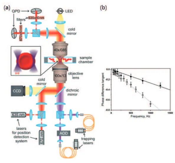
the cell when one edge of the cell is trapped and the other edge is oscillated by a vibrating beam in the optical tweezers [45]. In the experiment, two collimated single-mode lasers at the wavelength of 980 nm for trapping the cell and two other laser beams at wavelengths of 635 and 670 nm for detecting cell’s position are focused into the cell by the objective, as shown in Fig. 1.7(a). Another objective is used to collect the forward-scattered light and two quadrant photodiodes (QPDs) are employed to extract the local displacements of the cell sample during manipulation. The backward-scattered light by the trapped cell is sent into the CCD camera. In the dynamic testing, one trapping beam is stable while the position of the other beam is oscillated at a small amplitude in space, as shown in Fig. 1.7(a). The sinusoidal oscillating frequency is controlled by AOD and varies in the range from 50 Hz to 1 kHz. Lyubin et al recorded the phase differences between the cell displacement at the stably trapped side and the external perturbation of the oscillated trapping beam at each

frequency. The different mechanical properties of the abnormal cells could be distinguished from those of the normal cells via the comparison of the phase shift tangent, as shown in Fig. 1.7(b) [45].

Figure 1.7 Optical trapping system for dynamic testing and loss tangent measurements

Schematic diagram of the dual-trap optical tweezers for dynamic testing (a); phase shift tangent as a function of frequency (b). Empty points present the normal erythrocytes and filled points are for the cells fixed by glutaraldehyde. Grey and black lines are the linear mean-square fits to the data [45].

Optical traps generated by using the intrinsic astigmatism of the diode laser have been proved to realize the dynamic testing so that the cells could be sorted by their distinguished

viscoelastic responses in a high-throughput flow cytometry [35]. The dielectric objects manipulated by the astigmatic beam could only move along the beam axis and is trapped perpendicular to the beam axis because of the ravine-shaped potential landscape of the optical traps, as shown in Fig. 1.8 [47]. Theoretical analysis of the optical traps has been performed by the ray-tracing method by calculating the optical radiation forces distributions on the round surface of the cell [48-50]. In the experiment, the astigmatic beam of the diode laser at the wavelength of 810 nm is used to trap the RBC with an objective with 0.85NA (different from the commonly used highly focused and oil immersed objective) after passing through a 0.45NA objective and being reflected by a dichroic mirror, as shown in Fig. 1.8 [35]. The trapped sample is illuminated by the LED white light with the condenser lenses and another objective, and the images are collected with the trapping objective of the backscattering microscopy and sent into the COMS camera through the same dichroic mirror. The laser intensity is oscillated by a frequency generator [35]. The original oscillations of the trapping beam and the forced oscillated responses of the cell are recorded simultaneously on the computer. The phase delay, between the oscillated responses of the cell deformations and the frequency generator at a certain frequency, is obtained to characterize the viscoelastic properties of the cell in the frequency domain [39]. Sawetzki et al tested the cell elongation and the phase shift at the frequency higher than 5 Hz for the non-equilibrium cell deformation of the healthy and malaria-infected human erythrocytes for comparison [35]. The results indicate that the phase shift tangents of the malaria-infected cells are obviously different from the uninfected cells. On the other hand, as shown in Fig. 1.9, the scattered plot of the measured deformation of both infected and uninfected cells overlaps at frequencies higher than 5 Hz. On the other hand, the cell elongations of both infected and uninfected cells are different at frequencies lower than 2 Hz, and they seem like creep behaviors [35]. Therefore, as an additional cell mechanical biomarker, the dynamic testing for viscoelasticity could be used to characterize and screen cells at much faster timescales than the creep testing and the final

deformation measurement in the equilibrium state.

Figure 1.8 Dynamic testing of the high-throughput flow cytometry

Schematic of the high-throughput flow cytometry with optical traps (a). illustration of the deformed cell trapped by the optical forces [35].

Measured distributions of cell elongation (a) and phase difference between oscillated laser and cell deformations (b) of both infected and uninfected erythrocytes at frequencies higher than 5 Hz [35].

1.3.

Theoretical analysis of electromagnetic field

In order to quantify the mechanical properties of cell, the cell deformation under the optical tweezers with microbeads contact has been studied using the FEM [21, 41] and with the spectrin network model [51, 52]. However, the numerical analysis for the whole physical process of the direct manipulation of the biconcave cell by the optical trapping beams has not been reported in the literature. Direct trapping and manipulating a cell by the optical tweezers without mechanical contact to the cell was first demonstrated by Ashkin in 1987 [25]. Due to the 3D shape complexity of the cell and the limitation of the traditional ray-optics method [53], the analysis for a biconcave erythrocyte trapped by the optical tweezers directly has not been reported, although the analysis of a spherical microbead trapped by the focused laser beam has been well known. Fortunately, the computational models of finite-difference time-domain method (FDTD) [54], vectorial diffraction method [55], and FEM [37] provide solutions for calculating the light scattering with respect to the 3D shaped cell. Most of them, however, did not deal with side-incidence to the cell, nor with the focused laser beams, as that in the optical tweezers [56, 57].

To investigate the interactions between the cell and the optical trapping beams, our analysis involves multidisciplinary fields (e.g. electromagnetics, solid mechanics, and FEM). Meanwhile, the biological cell is approximated as a homogeneous isotropic material with the biconcave shape. In this section, the electromagnetic theory of the optical trapping and the radiation force of the optical field are described. The full 3D simulations and modeling with FEM for the light scattering and the final deformation of the biconcave-shaped erythrocyte in the dual-trap optical tweezers are introduced in Chapter 2 [58].

1.3.1.

Electromagnetic field of trapping beams

First, we modelled the vector field of the high NA trapping beams [58]. The conventional Gaussian beam is a paraxial solution of the scalar Helmholtz equation and is not appropriate for describing the high NA laser beam. The vector Gaussian beam with high order corrections can describe accurately the tightly focused beam. The solution as a series of the vector spherical wave functions with the expansion coefficients computed with the point matching method in the T-matrix method is described in [59]. However, a higher NA beam needs a higher order correction, but a higher order correction solution diverges at a shorter distance from the beam axis. For instance, a beam of NA = 1.25 requires the 7th order corrections, which converge within a distance of only 0.5λ from the beam axis [59] where λ = 1.06 µm is the wavelength of the beam. Therefore, this method would not be able to compute the trapping field on the surface of a biological cell of 5-10λ size.

Therefore, we define the trapping beam as a spherical beam with the Gaussian intensity distribution in the cross sections [42]. When two parallel beams travel along –z-axis with a certain separation distance S in x-direction, the complex amplitudes of the trapping beams are defined as

(

)

(

)

2 _{2 2 1/2} 1,2 2 _{2 2 1/2} 2 ( , , )exp [ 2 ] 0 ( , , ) 2 ( , , )exp [ 2 ] 0 A x y z j x S y z z E x y z A x y z j x S y z z

π

λ

π

λ

   ± + + >       =    _{− ± + +  <}  _{ }  (1.1)

which is the complex amplitude of the Gaussian beam A(x,y,z) with the phase of spherical wavefront as the exponential term with the wavelength λ. The beams are convergent when z > 0 and divergent when z < 0, and focused in the plane z = 0. As one solution of the paraxial Helmholtz equation, the complex envelop of the Gaussian beam is [60]

( )

( )

2 2 2 2 0 0 2 ( 2) ( 2) ( , , ) exp exp ( ) 2 ( ) W x S y x S y A x y z A jk j z W z W z R z ∗  ± +   ± +  = −  _− + Θ _       (1.2) where A0 is a constant,             = − n NA W 1 0 sin tan

π

λ

is the beam waist with the numerical

aperture NA= n⋅sin

θ

with the tangent of the divergence angle

0 tan W

π

λ

θ

= , n is the refractive index, λ π 2 0 0 W

z = is the Rayleigh range,

2 / 1 2 0 0 1 ) (               + = z z W z W is the beam radius, 2 0 ( ) 1 z R z z z  _{ }    = +       

is the wavefront radius of curvature, and 1

0 tan z z −   Θ =     is the phase retardation [60]. Thus, the electric field of the optical trapping beams Ei(x,y,z) (i =

1 or 2) could be written as

( )

(

)

( )

(

)

2 2 2 2 2 1/2 0 0 2 1,2 2 2 2 2 2 1/ 2 0 0 2 ( 2) 2 exp exp [ 2 ] 0 ( ) ( , , ) ( 2) 2 exp exp [ 2 ] 0 ( ) W x S y A j x S y z z W z _{W z} E x y z W x S y A j x S y z z W z W z π λ π λ   _{± +}  _{ }  ₋   _{± + +}  _>         =    _{± +}   − − ± + + <              (1.3)

where the phase term of the Gaussian beam in the Eq. (1.2) is replaced by the phase of the spherical wave when the Gaussian beam is highly focused by the 1.25 NA objective. The constant A0 related to the beam power P depends on the Poynting vector S whose

magnitude is 1 2

0 2 0 0 0 2

I _{= =} E H∗ ₌ A η

S with the ratio between the amplitude of the

electric and magnetic fields

n n n c k H E ₀ 2 / 1 0 0 0 0 0 0 0

ε

_η

η

µ

µ

ωµ

= =       = =

= , the total power

(

2

)

0 0 0 1 2 2

the radial distance of the beam

₍

₂

₎

2 2

x S y

ρ

= ± + where ω is the angular frequency, µ0

is the magnetic permeability, k is the magnitude of the wave vector, c0 is the speed of light in vacuum, ε0 is the electric permittivity, η is the impedance of the medium, and

Ω ≈ ≈       = 120 377 2 / 1 0 0 0

π

ε

µ

η

is the impedance of the free space [61, 62]. Thus, we have

0 0 0 1 480 2 P A I W n

η

= = and Eq. (1.3) becomes:

( )

(

)

( )

(

)

2 2 2 2 2 1/2 2 1,2 2 2 2 _{2 2 1/2} 2 480 1 ( 2) 2 exp exp [ 2 ] 0 ( ) ( , , ) 480 1 ( 2) 2 exp exp [ 2 ] 0 ( ) P x S y j x S y z z n W z W z E x y z P x S y j x S y z z n W z W z π λ π λ   _{± +}  _{ }  −   ± + +  >         =    ± +   − − ± + + <      _{ }       (1.4)

The beam polarization is in the plane normal to the wave vector of the spherical wavefront, which is defined as the radial polarization in this model. Figure 1.10 shows the scheme of the geometric relation between the wave vector k and the electric field E as well as the polarization components of E. In terms of two trapping beams focused at points (±S/2, 0, 0), three components of the electric field are expressed as

1,2 1,2 1,2 1,2 1,2 1,2 1,2 1,2 1,2 1,2 1,2 cos sin cos cos sin x y z E E E E E E φ θ φ θ φ = = = (1.5)

with the zenith angle

(

)

1 2 _{2 2} cos 2 i z x S y z

φ

− =

± + + and the azimuth angle

1 2 tan i x S y θ ₌ − ± .

Figure 1.10 Scheme of the radial polarization of the spherical wavefront

1.3.2.

Optical radiation force

The radiation force distribution at the cell/buffer interface could be computed as the inner product of the Maxwell stress tensor and the unit normal vector of the interface nr, as

described in chapter 2. The expression of the force is deduced as

2 2 2 2 2 2 1 1 2 2 1 1 2 2 2 2 2 2 1 1 2 2 1 1 2 2 1 1 2 1 1 2 [( ) (1 2)( )] (1 2)[( ) ( )] (1 2)( )[( ) ] n n n n t t n t E E E E n E E E E n E E n

σ

ε

ε

ε

ε

ε

ε

ε

ε

ε

ε

ε

ε

= − − − = − − − = − + r r r r (1.6)

where E1n and E1t are the normal and tangent components of the electric field, respectively. We have

(

E n E n

)

x

(

E n E n

)

y

(

E n E n

)

z n n n E E E z y x n E E _{y z z y z x x z x y y x} z y x z y x t ˆ ˆ ˆ ˆ ˆ ˆ − + − + − = = × = r r r with the complex values E_t E_yn_z E_zn_y

of the tangent component is ˆ+ ˆ+ ˆ

x y z

t t t t

E =E x E y E z

r

. The normal component of the electric field is

E

_n

=

E n x E n y E n z

_{x x}

ˆ

+

_{y y}

ˆ

+

_{z z}

ˆ

r

, with the complex valued components of

x n x x

E

=

E n

, y n y y

E

=

E n

, and z n z z

E =E n . According to Eq. (1.6) the radiation stress in the isotropic media is always normal to the interface, and the stress can be computed from the normal and tangent components En and Et of the electrical field in one medium only. Based on these expressions for the parameters in the electromagnetic field, the optical stresses or radiation forces applied on the 3D cell could be computed.

1.4.

Modeling methods quantifying mechanical properties of cells

Computational approaches play an important role in not only understanding of experimental trends but also providing new insights into the connection between cell mechanics and cell functions [63, 64]. When the smallest length scale of the concerned mechanical response of the cell is larger than the length over which the morphology and properties of the cell change, the modeling of continuum mechanics is generally applicable. The continuum-mechanics based FEM is the most common technique for investigating the biomechanics, in which the 3D multiple-layered model could be calculated with both material and geometrical nonlinearities [65, 66]. The 3D calculation with the FEM provides a useful tool to compute both static and time-dependent mechanical responses of the structured object applied either by the external loadings with attaching microbeads trapped by the optical tweezers [21, 66] or by optical radiation forces directly without attaching microbeads [37, 58]. With the help of the computational development, the modeling for the single biological cell could be built and solved to investigate the scattered electromagnetic field around and inside the cell [37, 57, 58], the stress distribution on the cell surface by the scattered light [54, 57, 67], the cytoskeletal mechanics [68], the fluid-structure interaction [65, 69], the viscoelasticity of the cell [70, 71], and the final deformation of the cell [37, 58,

72]. The modeling for quantifying the mechanical properties of the deformable materials are described below.

1.4.1.

1D viscoelastic model

Viscoelasticity is a time-dependent mechanical property of the material and contains both elastic and viscous characteristics. Testing the viscoelastic properties of the biological cell is of great interest for its intrinsic mechanical properties in the case that the cell is applied by the external loading. This is the microrheological technique [73]. Generally, there are a few typical viscoelastic behaviors, e.g. creep, recovery, relaxation and dynamic behaviors, with respect to different stimulations on the viscoelastic object. In order to quantify the viscoelastic properties with the constitutive equations we describe these behaviors, respectively.

1) When a loading stress is suddenly applied to the viscoelastic object at time t0 and kept constant afterward, the time-dependent deformation of the object follows a creep process, as illustrated in Fig. 1.11(a). The upper curve in green presents the loading stress versus time while the lower curve in purple is the strain as a function of time. The strain of the loaded object is jumping to a certain magnitude instantaneously at time t0 and increases exponentially afterward.

2) When a loading stress is suddenly released at time t0, the strain is jumping down instantaneously and exhibits a recovery or a progressive decrease of the deformation. This is the recovery process, as shown in Fig. 1.11(b).

3) Relaxation is the time-dependent decay of the stress when the strain or deformation of the object is held constant. Figure 1.11(c) shows the strain and stress relaxation behaviors in blue and red color, respectively.

4) The response of viscoelastic object to the sinusoidal load is referred to as the dynamic behavior of viscoelastic materials, as shown in Fig. 1.11(d). The upper curves are the sinusoidal stress and strain versus time with a time delay between the stress and the strain. The lower ellipse represents the hysteresis loop in each cycle of the loading oscillation, whose physical meaning will be discussed in Subsection 1.4.1.1. In order to quantify and predict the viscoelastic responses of biological objects to a loading stress or a certain deformation history, we will describe the commonly used models that could incorporate these typical responses. The inertia and resonant effects of the models which we analyze in the thesis are neglected.

Figure 1.11 stress-strain behaviors of viscoelastic testing methods

Stress and strain versus time for creep (a), recovery (b), relaxation (c), and dynamic behavior in sinusoidal loadings and its hysteresis loop [74](d).

1.4.1.1.

Spring-dashpot model

The linear viscoelastic behavior containing both elasticity represented by the springs and viscosity represented by the dashpots is often modeled by the combination of springs with elastic modulus E and dashpots with viscosity η [38, 39, 75, 76]. The instantaneous deformation generated by the spring is proportional to the load, while the displacement velocity represented by the dashpot is proportional to the load [38]. The spring-dashpot model is found to be useful to predict the viscoelastic behavior even though the real viscoelastic materials in general do not contain any springs and dashpots [24, 32, 45, 77]. There are a number of systematically series-parallel combinations of spring-dashpot models

[78]. Figure 1.12 shows the Kelvin (also called Voigt), Maxwell and Generalized Maxwell models, respectively. The Kelvin model is composed of a spring and a dashpot in parallel, as shown in Fig. 1.12(a). Both branches undergo the same deformation or strain and the total stresses are the sum of the stresses in each branch. The Maxwell model consists of a spring and a dashpot in series, as shown in Fig. 1.12(b). The stresses for both elements are the same but the total deformations or strains are the sum of the strains in each element. The Generalized Maxwell model consists of M + 1 branches in parallel with one main elastic branch of the spring elastic modulus G and M parallel Maxwell branches of the spring modulus Gm and the viscosity ηm (or the relaxation time τm) to fit various stress and

strain relations in the. The Generalized Maxwell models involves more exponential behaviors in creep, relaxation and recovery observed in the experimental results, as shown in Fig. 1.12(c) [79]. However, the generalized Maxwell model contains a series of elastic and viscous parameters which are to be quantified in experiment. Thus, this model provides more degrees of freedom in the simulations. The standard linear solid (SLS, also called Zener) model, composed of one Maxwell branch and one spring in parallel as shown in Fig. 1.13, is often preferred in realistic testing for biological cells [80, 81].

Figure 1.12 Schematic diagrams of spring-dashpot models

Figure 1.13 Schematic of SLS model

The viscoelastic responses could be obtained by the constitutive equation of the spring-dashpot model with a certain combination of springs and dashpots. Here we take the SLS model as an example to deduce the constitutive equation and to explain the viscoelastic behaviors shown in Fig. 1.11. In the SLS model, the total stress is the sum of that in each branch,

σ

=

σ

1 +

σ

2 with the stress of each spring

σ

1 and

σ

2. In the Maxwell arm, spring 1 and dashpot 3 receive the same stress

σ

1 =

σ

3. The stress and strain relations of each element are:

σ

₁ =E_{1 1}

ε

,

σ

₂ =E_{2 2}

ε

, and

σ

₃ =

η ε

_{3 3}& with the viscosity η₃, the elastic modulus E1 and E2, the strain of each element

ε

1,

ε

2, and

ε

3 and the strain rate

ε

&₃= ∂

ε

₃ ∂t. The total strains are

ε

=

ε

2 =

ε

1 +

ε

3. We obtain the constitutive equation in terms of the relations between stresses and strains for the SLS model:

(

)

3

E

1 3

E

1

E

2

E E

1 2

η σ

&

+

σ η

=

+

ε

&

+

ε

_(1.7)

The creep, recovery, relaxation and dynamic behaviors with the given stress or strain could be described by solving Eq. (1.7). The governing equation for the dynamic behavior could also be deduced from the Prony series in the generalized Maxwell model [82]. Therefore, by using the initial condition at time t0,

ε σ

=

a

(

E

₁

+

E

₂

)

with the constant stress σa as shown in Fig. 1.11(a), the strain function for creep is:

( )

(

)

( ) ( ) 1 2 0 3 1 2 1 2 1 2 2 E E t t E E a aE t e E E E E η σ σ ε − − + = − + (1.8)

The strain response of creep shows an upward jumping amplitude of

σ

a

(

E

₁

+

E

₂

)

at time t0 followed by an exponential increasing as shown in Eq. (1.8).

In the recovery behavior, the stress is at a value of σb and then suddenly released to zero at

time t0, as shown in Fig. 1.11(b). Based on the initial condition that at time t0 the strain is first jumped by an amplitude of

ε σ

=

b

(

E

₁

+

E

₂

)

, and then follows the solution of the differential equation of Eq. (1.7) as

( )

(

)

( ) ( ) 1 2 0 3 1 2 0 1 2 E E t t E E b t e E E η

σ

ε

ε

− − +   = −  +   (1.9)

Thus, the strain experiences a downward jumping amplitude of

σ

b

(

E

1

+

E

2

)

followed by

an exponential decreasing.

If the strain is kept constant at ε0 from time t0, the corresponding stress is deduced as:

( )

(

)

( ) 1 0 3 0 2 1 1 2 E t t t E E e E E η

σ

σ

= _ + − − _ + _{ } (1.10)

with the initial condition that

σ

0

=

ε

0

(

E

1

+

E

2

)

at time t0, as shown in Fig. 1.11(c).

Equation (1.10) describes the stress behavior of an exponential decrease from time t0 for the relaxation behavior. Among Eqs. (1.8-1.10), there exists a time-dependent exponential term with special parameters referred to as the recovery time (also as creep time or retardation time)

τ

σ

=

η

3

(

E

1

+

E

2

)

E E

1 2, and the relaxation time

τ

ε =

η

3 E1 in the SLS model [38,

39].

In the dynamic testing of the viscoelastic object, both loading stress and strain responses are sinusoidal as a function of time with a time delay ∆t, as shown in Fig. 1.11(d). The dynamic stress-strain relation can be written as:

( )

( )

( ) 0 i t t E e ω δ

σ

∗

ω ε

+ = (1.11)

where E∗=E′+iE′′ is the complex modulus, ε0 is the amplitude of the oscillated strain, and

ω

=2 f

π

is the angular frequency with the oscillation frequency f, the phase shift

t

δ

= ∆

ω

, and the real and imaginary modulus E’ and E”. Noting that in the dynamic testing of viscoelasticity, the phase shift tangent (also called the loss tangent) tanδ is an important parameter measuring the viscoelastic properties and is the ratio of the imaginary part of the modulus to the real part of the modulus [74]:

[

]

[

]

" 1 ' 2 2 1 tan 1 ( ) ( ) 1 1 (1/ K) 1/ (K ) E E E E E σ σ σ σ σ

ωτ

δ

ωτ

ωτ

ωτ

ωτ

≡ =  ₊ ₊   = + + (1.12)

with the ratio K = E1/E2. In addition, the loss tangent can also be computed from the elliptic stress-strain relation, the hysteresis loop, as shown in Fig. 1.11(d) [74]. This geometrical relation of the loss tangent in the hysteresis loop, tanδ = OA/OB, provides an alternative way to quantify the viscoelasticity [74].

1.4.1.2.

Power-law model

In the creep testing, the power-law model is another way to describe the viscoelastic behavior with the material deformation d and time t [83, 84]. As a simple empirical equation, the creep function J(t) of the power-law model is written as [83]:

( )

( )

0

(

0

)

J t =d t F = j t

τ

β (1.13)

characterizing the softness or the compliance of the material. Time is normalized by the timescale τ0 in the range from 0 to 1. The power-law exponent β is not relevant to the value of τ0. If the power-law exponent β is close to zero, Eq. (1.13) describes the purely elastic solid; if β is close to one, Eq. (1.13) denotes the purely viscous fluid. A higher value of β leads to a more dissipative behavior [83]. In the dynamic testing, the power-law rheology model can also be used to predict the viscoelasticity of the soft glassy materials [83] by taking the mathematical manipulation proposed in the literature [84].

It is necessary to compare the single exponential of the spring-dashpot model and the power-law model, one of which is chosen to estimate the viscoelastic properties of biological cells [24, 45, 70]. For comparison, we take the relaxation behavior as an example to plot the modulus E(t) versus time t on a linear time scale over a decade in Fig. 1.14(a) and on a logarithmic time scale over seven decades in Fig. 1.14(b). The exponential relaxation modulus

E t

( )

= +

1 exp

( )

t

is represented in the blue solid curve and the power-law relaxation modulus

E t

( )

=

1.3

t

−0.17 is plotted in the red dash line. It is noted that two curves are similar on a linear time scale while they differ a lot on a logarithmic time scale [39]. According to the special mathematical features of these two viscoelastic models, the time-dependent or frequency-dependent mechanical responses of the object are recorded in experiment and fit via the appropriate theoretical model to obtain the mechanical properties of the biological materials.

M

o

d

u

lu

s

E

(t

)

Time t

1.3t-0.17 10-3 10-2 10-1 100 101 102 103 104 0 1 2 3 4 5 1+exp(-t) 0 1 2 3 0 1 2 3

M

o

d

u

lu

s

E

(t

)

1.3t-0.17

Time t

1+exp(-t)

(a)

(b)

Figure 1.14 Time-dependent mechanical modulus

Illustration of single exponential and power-law relaxation on a linear time scale over one decade (a) and on a logarithmic time scale over seven decades with arbitrary units of modulus and time (b).

1.4.2.

3D multi-layer model

In order to quantify the mechanical properties of the biological cell based on the continuum mechanics, the 3D models have been developed. The cellular mechanics research on the human RBC has always been a topic for a number of biomechanics literatures [38, 85-87]. The human RBC membrane, composed of the phospholipid bilayer, the cytoskeleton and transmembrane proteins, plays an important role in not only supporting the cell morphology but also dominating the consequent deformation of the cell under the external force. The cell membrane is commonly modeled as the effective continuum shell with a certain thickness as shown in Fig. 1.15. In the case of the small deformation, the cell is generally modeled as the linear elastic material for fitting to the final deformation, or the linear viscoelastic material for fitting to the time dependent cell deformation. In the case of the large deformation (more than 10% elongation), the hyperelastic material can be used to model the cell membrane with nonlinear mechanical responses to the loading forces. In this section, three types of the membrane models with the viscous cytosol are introduced.