Economic Relevance of Hidden Factors in International Bond Risk Premia

Economic Relevance of Hidden Factors in

International Bond Risk Premia

Luca TIOZZO ”PEZZOLI”

∗

First version : April, 2013.

This version: April, 2014.

Abstract

This paper investigates the relevance of hidden factors in international bond risk premia to forecast future excess bond returns and macroeconomic variables such as economic growth and inflation rate. Using maximum likelihood estimation of a linear Gaussian state-space model, adopted to explain the dynamics of expected excess bond returns of a given country, associated selection criteria detect as relevant, factors otherwise judged negligible by the classical explained variance approach adopted by

Cochrane and Piazzesi(2005) andCochrane and Piazzesi (2008). We call these factors hidden, meaning that they are not visible through the lens of a principal component analysis of expected excess bond returns. We find that these hidden factors are useful predictors of both future economic growth and inflation rate given that they add forecasting power over and above the information contained both in theCochrane and Piazzesi(2008) and in yield curve factors. These empirical findings are robust across different sample periods and countries as well as with respect to the interpolation technique used in the construction of the international bond yield data sets.

Keywords: financial econometrics, interest rates, international finance.

JEL classification: C52, E43, G12, G15.

∗_{Universit´e Paris-Dauphine, DMR Finance - CEREG - Place du Mar´echal de Lattre de Tassigny 75775}

Paris Cedex 16 [E-mail: luca.tiozzo.p@gmail.com] and Universit´e Paris I - Panth´eon Sorbonne, 17, Rue

de la Sorbonne, 75005 Paris [E-mail: luca.TIOZZO-PEZZOLI@univ-paris1.fr].

When writing this paper, I have benefited from discussions with Fulvio Pegoraro at Banque de France

and Andrew Siegel. I will thank Jean-St´ephane M´esonnier and Benoit Mojon at the Bank of France. I

will also thank B´eatrice Saes-Escorbiac, Aur´elie Touchais and Guilleume Retout for excellent research

assistance. I am grateful to participants at the Computational and Financial Econometrics Conference (CFE 2013) in London, ADRES Doctoral Conference in Economics at Dauphine University in Paris, the Mathematical and Statistical Methods for Actuarial Sciences and Finance Conference (MAF 2014) in Salerno, for helpful discussions and comments on previous versions of this paper. Any remaining errors are mine. The views expressed in this paper is mine and do not necessarily reflect the views of the

1

Introduction

The bond risk premia literature has focused not only on the problem of detecting factors to forecast future excess bond returns but it has also considered the problem of predicting important macroeconomic

variables such as the economic growth [seeKoijen, Lustig, and van Nieuwerburgh (2012) and Dahlquist

and Hasseltoft(2013), among others].

In the first case,Cochrane and Piazzesi (2005) andCochrane and Piazzesi (2008) have found that

the tent shaped factor accounting for almost all the variability in (expected) excess bond returns (in the

U.S. economy) is also a relevant predictor for them. Recent papers byKessler and Scherer (2009) and

Sekkel(2011), extending the analysis ofCochrane and Piazzesi (2005) andCochrane and Piazzesi(2008) outside the U.S. economy, confirm the presence of one single return-forecasting factor in international bond markets. However, we conjecture a possible weakness behind their analysis given that, according to

Duffee(2011), the methodology used in the extraction of factors is crucial to judge their importance from

a time-series (forecast) perspective. More precisely,Duffee(2011) uses a Kalman filter-based maximum

likelihood approach to estimate a five-dimensional Gaussian affine term structure model and he detects a factor which is found to be a good predictor of both the short rate and bond returns, even if it is hidden in the cross section of yields, being the associated explained variance negligible. In other words, we may have factors with a small explained variance but showing, at the same time, an important forecasting power about excess bond returns.

In the second case, several studies [seeCochrane and Piazzesi(2005),Koijen, Lustig, and van

Nieuwer-burgh (2012), Dahlquist and Hasseltoft (2013), among others] have investigated the link between the return-forecasting factor and economic growth for the U.S. and for several developed countries. In gen-eral, they find that this factor is countercyclical and contains information about future economic growth while the relationship with inflation is ignored, given that it is the yield curve level, and not excess bond

returns, seems as related to inflation [seeAng and Piazzesi(2003),Diebold, Li, and Yue(2008),Cochrane

and Piazzesi(2005) and Cochrane and Piazzesi (2008)]. However, as mentioned above, information in hidden factors could help in predicting economic growth and could disclose some forecasting power for inflation as well.

The purpose of this paper is to fill this gap in the literature by investigating the relevance of factors hidden in international bond risk premia to forecast future excess bond returns as well as macroeconomic variables such as economic growth and inflation rates. We propose, using maximum likelihood (ML) cri-teria and parameters significance, within a linear Gaussian state-space approach, to estimate and select a preferred number of factors to explain expected excess bonds returns in four leading bond markets (namely, the U.S., U.K., German and Japanese bond markets). Then, these factors are used to predict excess bond returns, economic growth and inflation rates.

Our choice of a linear Gaussian state-space approach is important at least for two reasons. First, the Kalman filter-based maximum likelihood estimation of the state-space model might judge as important factors otherwise seen as negligible when the standard explained variance methodology is used. Second, the large time-series and cross-sectional dependence of bond returns and the typical small dimension of its maturity spectrum prevent us from successfully applying selection criteria of factor model analysis in

order to detect the number of factors required to explain bond risk premia [see, among the others, Bai

This paper is organized in two parts. In the first part, autoregressive stationary latent factors are used within our linear Gaussian state-space approach in order to explain expected excess bond returns for each of the four bond markets. We consider alternative model specifications characterized by a number of

factors going from one, as inCochrane and Piazzesi(2005) andCochrane and Piazzesi(2008), to five, as

suggested by the recent term structure literature [Adrian, Crump, and Moench(2013) andDuffee(2011)].

Maximum likelihood estimation of the state-space model is performed by using the EM algorithm with

Kalman Filter and Kalman Smoother recursions [Engle and Watson (1981), Quah and Sargent (1993)

andDoz, Giannone, and Reichlin(2011),Doz, Giannone, and Reichlin(2012)]]. We derive forward rates and construct expected excess bond returns by using the international Treasury yield curves database ofPegoraro, Siegel, and Tiozzo Pezzoli(2012), observed monthly from January 1, 1986 to December 31, 2009. We select the preferred number of factors by means of maximum likelihood criteria, namely the

bootstrap variant of Akaike Information Criteria (AICb) of Cavanaugh and Shumway (1997) and the

significance of parameters by performing a Nonparametric Monte Carlo bootstrap for state-space models of Stoffer and Wall (1991). The kind of bootstrap we adopt is a block stationary bootstrap able to

properly taking into account the persistence of bond returns [Politis and Romano(1994) andPolitis and

White(2004),Patton, Politis, and White (2009)].

Given our extracted factors, in the second part of the paper we investigate their relationships with future excess bond returns and macroeconomic variables. More precisely, we first evaluate the prediction of future excess bond returns by running regressions of one-year excess bond returns on the extracted factors and then, we check the contribution of the latters in forecasting both industrial production growth and inflation rates. Finally, we compare our results with competitors in the literature.

Our empirical analysis suggests that a state-space model with five factor is generally preferred. How-ever, only one factor is statistically important to predict future excess bond returns and it closely tracks the return-forecasting factor. As a matter of fact, it seems that factors that marginally contribute to explain the variance of expected bond returns, are not useful in predicting them. Conversely, when we evaluate their contribution in predicting future macroeconomic variables in each economic area, we un-cover an appealing result. More precisely, factors usually seen as capturing only idiosyncratic movements in bond returns, reveal to be important predictors for both economic growth and inflation rates. They add an incremental forecasting power over and above the information contained in both the return-forecasting

factor and yield curve factors [seeAng and Piazzesi(2003),Diebold, Li, and Yue(2008)]. In other words,

after having controlled for the forecasting power contained in the yield curve slope (level, respectively),

we calculate the difference in percentage points (DP P ) between the (adjusted) R2 of predictive

regres-sions of future industrial production growth (inflation rates, respectively) using our extracted factors and regressions which use the return-forecasting factor and yield curve factors instead. We evaluate these differences for forecasting horizons up to three years. Finally, we calculate the average difference across forecasting horizons (ADDP ) and we construct a measure that we call, for the industrial production

growth, ADP Pg and, for inflation rates, ADP Pπ. We find always positive values for the ADP Pg across

countries. They range from 14.6% in the U.K. to 3.2% in the U.S.. In Germany and Japan, we have

an ADP Pg of 6.6% and 4%, respectively. Our extracted factors play an important role in forecasting

inflation as well. The ADP Pπ is always positive and ranges from 11.2% in Japan to 2.2% in U.S.. In

Germany we obtain a value of 7% while in U.K. it is as big as 3.6%.

In order to check that these results are not due to the adopted sample period, to the market analyzed or to the interpolation technique used in the construction of forwards rates we perform a battery of

robustness checks. We estimate state-space models by using international data from different sources

[namely, Wright (2011), Fama and Bliss (1987)] and for different sample periods by adopting both an

increasing and a rolling window of observations in the estimations. Our main conclusions do not change: hidden factors are important predictors of economic growth and inflation rates across markets and sample periods and regardless the interpolation technique used in the construction of international data.

The paper is organized as follows. In Section 2 we introduce the bond notation, the typical

ap-proaches used in the literature in order to predict excess bond returns and macroeconomic variables and

we describe the state-space model used in the extraction of factors across different economies. Section3

presents the empirical analysis, starting with the data description in Section3.1and state-space models

estimations in Section 3.2 (for different countries and different number of factors). In Section 3.3 we

present the results of in-sample forecasting regressions for excess bond returns and in Section3.4the

in-sample forecasting regressions for the macroeconomic variables. Section3.5focus on robustness checks,

while Section4concludes.

2

Literature

2.1

Bond Notation

Let us define by p(n)_j,t the log-price at time t in a country j of a discount bond with a residual maturity n.

The relationship linking the log-price and the log-yield is:

y(n)_j,t = −1

np

(n)

j,t. (1)

The (short) log-forward rate f_j,t(n)at time t for loans beginning at time t + n − 1 and ending in t + n is:

f_j,t(n)= p(n−1)_j,t − p(n)_j,t. (2)

The log-return from buying at time t, a bond with residual maturity n and selling it, in t + 1, when its residual maturity is n − 1 is:

r(n)_j,t+1= p(n−1)_j,t+1 − p(n)_j,t. (3)

The log-return in excess over the one-year yield is:

rx(n)_j,t+1= r(n)_j,t+1− y_j,t(1). (4)

2.2

Bond Returns Predictability and the link with the

Macroe-conomy

Several empirical studies have shown that forward rates contain important information about future

excess bond returns. Fama and Bliss(1987), pioneers in this area of finance, use the spread between the

n. They run the following regressions:

rx_j,t+1(n) = α(n)_j + β(n)_j (f_j,t(n)− y(1)_j,t) + ε(n)_j,t+1, (5)

where j is the U.S. and obtain an R2 _{up to 14%. More recently,Cochrane and Piazzesi (2005) regress}

one-year excess bonds returns onto a constant and a set of forward rates:

rx_j,t+1(n) = β_j,0(n)+ β_j,1(n)y_j,t(1)+ β_j,2(n)f_j,t(2)+ · · · + β_j,k(n)f_j,t(k)+ ε(n)_j,t+1, = βjfj,t+ ε (n) j,t+1. (6) where ε(n)_j,t ∼ IIN (0, σ2(n)_j ), βj = [β (n) j,0, β (n) j,1, β (n) j,2, . . . , β (n) j,k] and fj,t = [1, y (1) j,t, f (2) j,t, . . . , f (k) j,t ]0 and k is the

biggest forward rates maturity available1 _{and country j is the U.S.. They find a suggestive tent-shape}

pattern characterizing the regression coefficients2 _{and detect a single-factor structure characterizing the}

bond risk premia at all maturities. In light of this result, Cochrane and Piazzesi (2005) describe the

one-year excess bond returns as follows:

rx(n)_j,t+1 = bj,n(γj,0+ γj,1y (1) j,t + γj,2f (2) j,t + · · · + γj,kf (k) j,t) + ε (n) j,t+1 = bj,n(γjfj,t) + ε (n) j,t+1, (7) where γj= [γ (n) j,0, γ (n) j,1, γ (n) j,2, . . . , γ (n) j,k] and 1 k−1 Pk

n=2bj,n= 1 [seeCochrane and Piazzesi(2005) for details].

They estimate the above regression in two steps. First, they regress the average (across maturities) excess bond return on the available forwards rates:

rxj,t+1 = γj,0+ γj,1y (1) j,t + γj,2f (2) j,t + · · · + γj,kf (k) j,t + εj,t+1, = γjfj,t+ εj,t+1, (8) where rxj,t+1= _k−11 Pk_n=2rx (n)

j,t+1. They then take the fitted values and construct the so called

return-forecasting factor or Cochrane and Piazzesi factor (CP factor, hereafter):

xj,t := γ_bjfj,t (9)

Second, they estimate bj,n by regressing the one-year excess bond returns on the CP factor, as follows:

rx(n)_j,t+1= bj,nxj,t+ ε

(n)

j,t+1, (10)

1_{In their case k is equal to five since they use Fama and Bliss(1987) forward rates from one to five}

years of maturity. In our empirical analysis, we consider the case where k is equal to five and nine.

2_{The pattern of coefficients seems to depend on the interpolation technique used in the construction}

of the forward rates [Dai, Singleton, and Wei (2004)]. Contrary to the unsmoothed techniques,

para-metric methods, such as the ones proposed by Nelson and Siegel (1987) and Svensson (1994), smooth

forwards rates across maturities. As a result, regression coefficients in (6) have a W-shape reflecting

strong multicollinearity between regressors. In order to overcome this problem,Wright and Zhou(2009),

Singleton (1978) and Sekkel (2011) use only three forward rates to explain the one-year excess bond

returns. Others, likeCochrane and Piazzesi (2008) regress the one-year excess bond returns calculated

using theGurkaynak, Sack, and Wright(2007) database onto a constant and the Fama and Bliss forwards

and they find an explanatory power for these regressions of 35% in the U.S3.

In some recent studies, this analysis has been extended outside the U.S.. For instance,Dahlquist and

Hasseltoft(2013) construct the CP factor and study excess bond predictability also in U.K., Germany and

Switzerland whileSekkel(2011) enlarge the analysis to nine developed countries in the data sets ofWright

(2011). Although they have found also that the CP factor is responsible of bond return predictability also

at an international level, some evidence of heterogeneity appears as well, since its performance depends upon the country and the adopted sample period.

More recently,Cochrane and Piazzesi(2008) have proposed another way to construct the CP factor

and show that it dominates the variance of expected returns. In practice, they calculate first expected excess bond returns:

Et(rx

(n)

j,t+1) = βbjfj,t. (11)

Afterwards, they conduct an eigenvalue-eigenvector decomposition of the covariance matrix of expected

excess bond returns so that QΛQ0 = cov[Et(rx

(n)

j,t+1)], where Q are the eigenvectors and Λ is the diagonal

matrix of eigenvalues. They define the CP factor as follows:

xj,t = q0τ[Et(rx

(n)

j,t+1)], (12)

where qτ is the eigenvector in the matrix Q corresponding to the largest eigenvalue in the matrix Λ.

This factor accounts for almost all (more than 99%) the variability in the expected excess bond returns, while the remaining ones are only responsible of idiosyncratic movements in each bond maturity and thus judged not economically meaningful.

They also use yield curve factors to predict excess bond returns:

rx(n)_j,t+1 = α(n)_j + β_j(n)Lj,t+ γ (n) j Sj,t+ δ (n) j Cj,t+ ε (n) j,t+1, (13)

where ε(n)_j,t ∼ IIN (0, σ2(n)_j ) and Lj,t, Sj,tand Cj,t are the level, slope and curvature factors, respectively.

They find that these three factors do not perform as well as the CP factor in predicting excess bond returns and therefore the CP factor is judged not fully spanned by the yield curve. This finding is

con-firmed outside the U.S. economy byDahlquist and Hasseltoft(2013).

From a macroeconomic perspective, the CP factor seems to contain important information about

future economic growth. In particular,Koijen, Lustig, and van Nieuwerburgh(2012) runs the following

regressions:

gj,t+h = αj,h+ βj,hxj,t+ εj,t+h, (14)

where εj,t ∼ IIN (0, σj2), h = 12, 18, 24, 30 and 36 months indicates the forecasting horizon, gj,t is the

date t economic growth measured by the Chicago Fed National Activity Index and country j is the U.S.. They find that the CP factor is a strong predictor of future economic growth at 12 and 24 months ahead.

In an international context,Dahlquist and Hasseltoft(2013) run regressions where the yield curve slope,

3_{This value rises to 44% if three-month moving averages of forward rates are adopted instead of}

the current one alone. They argue that measurement errors is the main cause for this increase in the performance.

Sj,t, is the only predicting variable for industrial production growth:

gj,t+h = αj,h+ γj,hSj,t+ εj,t+h, (15)

and regressions where the CP factor and the slope of the yield curve are both used as regressors,

gj,t+h = αj,h+ βj,hxj,t+ γj,hSj,t+ εj,t+h. (16)

They find that, at some forecasting horizons, both factors are statistically important in predicting future industrial production growth.

2.3

The state-space Approach

In this section we define the linear Gaussian state-space model that we adopt to describe the dynamics of expected excess bond returns of a given country. The model is specified by the following assumptions:

Assumption 1 (Expected Excess Bonds Returns and Latent Factors): We denote by Et(rx

(n)

j,t+1)

the n × 1 vector of expected excess bond returns observed at time t for country j. We denote by Fj,t the

k × 1 vector of latent factors at time t that explain expected excess bond returns, at all maturities, for country j.

Assumption 2 (The Single-Country Bond Risk Premia Model): For a given k-dimensional latent

factor Fj,t, the dynamics of expected excess bonds returns Et(rx

(n) j,t+1) is given by:      Et(rx (n) j,t+1) = µ + Λ Fj,t+ εt, εt∼ IIN (0, Ω) Fj,t = Φ Fj,t−1+ ηt, ηt∼ IIN (0, Ψη) , (17)

where µ is an n × 1 vector of constants, Λ is n × k matrix of factors loadings and Ω is the n × n

variance-covariance matrix of the Gaussian-distributed white noise εt. Φ is the k × k autoregressive matrix and

Ψη is a k × k identity matrix .

To efficiently estimate the model for expected excess bond return, for any given country, we follow

the EM-based recursive maximum likelihood estimation procedure adopted by Pegoraro, Siegel, and

Tiozzo Pezzoli (2013). While their methodology is adopted in a multi-country setting, here we want to explain the dynamics of expected excess bond returns in a single-country context. Following their

notation, our model has r(l)_{= 0, r}(c)_{= k, Λ}

l= 0 and ΛB= Λc = Λ.

3

Empirical Analysis

The purpose of our empirical analysis is to select the number of factors required to explain expected excess bond returns in four leading bond markets and then to evaluate their ability to predict industrial

production growth and inflation rates. The international data we use are described in Section3.1. Model

estimation results, adopting the estimation method of Section2.3, along with the selection of preferred

number of factors in each country, using the parameters’statistical significance and the bootstrap variant

in Section 3.2. In Section3.3 we assess excess bond return predictability while in Section3.4 we focus on industrial production growth and inflation rates. In all these cases, we compare predictions obtained using our extracted factors with the ones we get by competitors in the literature (CP and yield curve

factors). Finally, in Section3.5we run a battery of robustness checks in order to test whether our findings

depend on the adopted sample period, on the analyzed market or on the interpolation technique used in the construction of the international data.

3.1

Data

We use the international Treasury yield curve of Pegoraro, Siegel, and Tiozzo Pezzoli (2012), [PST

hereafter], consisting of four leading bond markets: the U.S., U.K., Germany, and Japan4_{. Yields are}

observed monthly, from January 1986 to December 2009.

We also consider data from other sources for robustness checks. In particular, for the U.S., we use

yield data ofWright(2011)5_{andFama and Bliss(1987). For Germany and Japan, we consider the term}

structures in the international database ofWright (2011)6_{. Finally, we use monthly data for industrial}

production and consumer price index taken from OECD and calculate the annualized growth in industrial production growth and inflation rates in each economic area.

3.2

Model Selection: State-Space and Principal Component

Fac-tors Selection

In this section we estimate model (17) for several k and select the preferred number of factors required

to explain expected excess bond returns in international bond markets. For any given country, we use the international yield curve database of PST, with residual maturity from one to nine years, to derive forward rates and construct expected excess bond returns. The latters are used to estimate the linear

Gaussian state-space model described in Section 2.3. Different model specifications characterized by a

number of factors going from 1, as inCochrane and Piazzesi(2005) andCochrane and Piazzesi(2008), to

5 factors, as suggested by the recent term structure literature [Adrian, Crump, and Moench(2013) and

Duffee(2011)] are considered. We also perform principal components analysis of expected excess bond

returns as inCochrane and Piazzesi(2005) andCochrane and Piazzesi(2008).

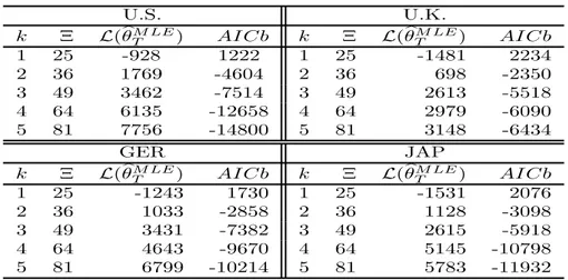
Table 1 provides the marginal and cumulative percentage of variance explained by factors extracted

from the covariance matrix of expected excess bond returns. Table2 reports the maximum value of the

log-likelihood function for each estimated linear Gaussian state-space model along with the value of the

AICb, while Table 3 shows the maximum likelihood estimates of the matrix loadings in Λ and of the

autoregressive coefficients in Φ as well as the associated bootstrap standard errors.

4_{The database is characterized by uniform level of liquidity and a (parsimonious smoothed)}

inter-polation technique for the discount function. More precisely, Treasury coupon bonds data are filtered

using theGurkaynak, Sack, and Wright (2007) criteria and the discount function is interpolated using

theNelson and Siegel(1987) methodology.

5_{Yield curves for the U.S. economy are taken fromGurkaynak, Sack, and Wright(2007).}

6_{In the Appendix8we also consider the international bond yields database kindly supplied byDiebold,}

Li, and Yue(2008). In this data set, term structures are estimated by means of the unsmoothed Fama and Bliss(1987) methodology.

As can be seen from Table1, the first principal component accounts for more than 95% of expected returns variance across bond markets suggesting a single-factor structure behind the international bond risk premia. However, when we consider maximum likelihood estimation results, additional factors seem

to help explaining expected returns. From Table2we notice a substantial rise in the log-likelihood values

when we increase the number of factors and, according to AICb, we systematically select the 5-factors

model. As suggested by the model selection literature [Linhart and Zucchini(1986)], we may make this

choice simply because this model has a larger factor’s dimension with respect to the competing ones. In order to understand if this specification is truly required by the data, we evaluate whether these factors are statistically important to explain the dynamics of expected returns across countries. Form a careful

inspection of Table3, we note that loadings in Λ are all statistically different from zero at 5% significance

level. We also find statistically significant coefficients outside the main diagonal of the matrix Φ thus suggesting causality between the estimated factors.

Clearly, the statistical approach adopted is relevant in the choice of the number of factors. Factors that we are tempted to consider responsible of only idiosyncratic movements on bond maturities, since they marginally contribute to explain the variance of expected returns, turn out to be important when we take

into account the dynamics (and persistence) in bond risk premia7_.

At this point of the analysis, we have shown that hidden factors, i.e. not detected by the classical principal components methodology, are clearly helpful in describing expected excess bond returns. In the next sections, we will study their contribution in predicting future excess bond returns and macroeconomic variables such as industrial production growth and inflation rates.

3.3

Predictability of Excess Bond Returns

In this section we present results from forecasting regressions concerning one-year excess bond returns. First, we consider classical predictors in the literature like the forward-spot spread, the CP factor and

yield curve factors. In practice, we run regressions (5), (10) and (13), for each analyzed country. Results

are reported in Table48_{. Then, we consider the following regressions:}

rx(n)_j,t+1 = bjFbj,t|T+ ε (n) j,t+1, (18) where bj = [b (n) j,0, b (n) j,1, b (n) j,2, . . . , b (n)

j,5] and ˆFj,t|T is our 5-dimensional vector of extracted smoothed factors

for country j. Table5shows the associated results.

Let us consider classical predictors first. Forward-spot spread provides the worst performances,

while regressions involving the CP factor supply the best ones across markets, and regression coefficients associated to this factor are statistically significant across countries. The three (level, slope and curvature) yield curve factors do not over-perform the CP factor but they do better than the forward-spot spread. Looking at the statistical significance of coefficients, we notice that the level does not help in predicting excess bond returns while the slope is important in Japan and, at long bond maturities, in Germany.

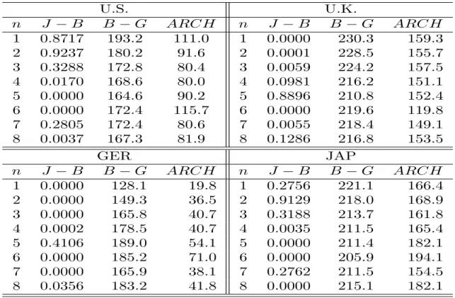
7_{Table19in the Appendix9provides residual analysis of regressions of expected excess bond returns}

at different maturities on the CP factor. Residuals are conditionally heteroskedastic, strong serially correlated and, at some maturities, far from normality.

8_{We do not show results concerning the CP factor calculated as in (12). The reason is that the}

correlation between factors calculated either following (9) or (12) is always above 0.99. As a matter of

Curvature is a statistically significant predictor both in U.K. and Japan.

As far as the five extracted smoothed factors are considered, only the first one reveals to be

statisti-cally important in describing future bond returns as highlighted in Table5. The only exception is Japan,

where the second factor presents statistically significant regressions coefficients at short maturities. The

R2of these forecasting regressions are close to the ones using the CP factor9unlike a slight improvement

for short bond maturities. However, 90 % confidence intervals for the R2 _{have slightly higher lower and}

upper bounds than other competitors in the literature10_.

From this analysis we conclude that the first one of the five extracted factors contributes to

fore-cast one-year excess bond returns. It produces R2 _{similar to the CP ones (the best predictor among}

competitors in the literature) with a slight improvement for short bond maturities and in confidence intervals.

3.4

Predictability of Macroeconomic Variables

3.4.1

Predictability of Economic Growth

In this section we present forecasting regressions results of industrial production growth, and we consider

forecasting horizons up to three years. We first run the classical regressions (14) and (15) to assess the

predictive power contained in the CP factor and the yield curve slope, and then we use both predictors

jointly by running regressions (16). Afterwards, we consider the following regressions:

gj,t+h = bj,hFˆj,t|T+ εj,t+h. (19)

where h = 12, 18, 24, 30 and 36 months indicates the forecasting horizon, bj,h= [bj,h,0, bj,h,1, bj,h,2, . . . , bj,h,5],

and ˆFj,t|T is our 5-dimensional vector of extracted factors for country j. In this case we also take into

account the predictability contained in the yield curve slope by running the following regressions:

gj,t+h = bj,hFˆj,t|T+ cj,hSj,t+ εj,t+h. (20)

where Sj,t is the yield curve slope.

Results from classical methods are presented in Table6, while the ones concerning our extracted factors

are provided in Table7.

Let us focus again on classical predictors first. When we adopt the CP factor and the yield curve slope as regressors, the former seems to provide additional information with respect to the latter at all forecasting horizons in U.K. (except for the 12 months) and at 12 and 18 months horizons in Germany. In Japan, it improves forecast precision till 24 months ahead. In fact, in all these cases, we observe

statistically significant coefficients associated to the CP factors yielding higher R2 with respect to the

case where the yield curve slope is the only predicting variable. In U.S. only coefficients associated to

9_{The first extracted factor closely tracks the CP one being the associated correlation above 0.98 across}

countries.

10_{Confidence intervals are calculated adopting the block stationary bootstrap method ofPolitis and}

Ro-mano(1994) andPolitis and White(2004). The blocks size is chosen followingPatton, Politis, and White

(2009). This procedure permits to properly taking into account the persistence and heteroskedasiticy of

the yield curve slope are statistically significant. Confidence intervals for the R2, in regressions where the slope of the yield curve and the CP factor are considered jointly, have higher lower and upper bounds than regressions considering these two factors separately.

Next, we consider our extracted factors as predictors of future industrial production growth. An

inspection of Table7highlights that, in all the bond markets considered, many predictability coefficients

associated to these factors are statistically significant even when we control for the forecasting power

provided by the yield curve slope. In this latter case, we notice higher R2 _{with respect to the classical}

case where the CP and the yield curve slope are considered jointly. For example, in U.S. we observe an

increase in the R2 from 6% and 11% to 11% and 15%, for predictions 12 and 18 months ahead,

respec-tively. In U.K., we notice a rise in the R2_{of 19% at 36 months horizon of 17% at 12 months horizon. For}

the other horizons, the average increment is around 12%. Also in Germany we observe, at all forecasting

horizons, a general improvement in the R2 _{but with a lower magnitude with respect to the case of U.K..}

Indeed, the best results are obtained at 12 and at 36 months horizons: the R2 rises from 13% and 16%

to 18% and 24%, respectively. Finally, also in Japan we gain in terms of explanatory power by using

our extracted factors. The peak is for forecasts 30 months ahead, where we move from a R2_{of 1% using}

the CP factor to 10% when the five extracted smoothed factors are adopted. Generally, lower and upper

bound on the 90% confidence intervals for the R2are higher in these regressions than the one using CP

factor and the yield curve slope as predictive variables.

To sum up results presented above, it is interesting to observe that our EM-based smoothed factors strongly help predicting industrial production growth and it outperforms the forecasting power of classical CP tent-shaped factor even when we control for the yield curve slope predictive power.

3.4.2

Predictability of Inflation

In this section, we present the results of forecasting regressions about inflation rates. Also in this case we consider forecasting horizons up to three years. We run five type of predicting regressions. First, we use the CP factor to predict future inflation rate as follows:

πj,t+h = αj,h+ βj,hxj,t+ εj,t+h, (21)

where εj,t ∼ IIN (0, σ2j,t), h is the forecasting horizon and πj is the inflation rate of country j. Second,

we evaluate the predictive power of the yield curve level of country j, Lj,t as follows:

πj,t+h = αj,h+ βj,hLj,t+ εj,t+h. (22)

Third, we consider the CP factor and yield curve level jointly as follows:

πj,t+h = αj,h+ βj,hxj,t+ γj,hLj,t+ εj,t+h. (23)

Fourth, we use our selected five smoothed factors:

where bj,h = [bj,h,0, bj,h,1, bj,h,2, . . . , bj,h,5] and, finally, we consider these five factors and the yield curve level jointly:

πj,t+h = bj,hFˆj,t|T+ γj,hLj,t+ εj,t+h. (25)

Given that excess bond returns are not related to inflation, considering the CP factor in the forecasting

regressions (21) and (23) may appear useless. However, this allow us to precisely assess the forecasting

power added by our extracted factors over and above the information contained in the return-forecasting factor.

Table8 shows that the variable which mostly matter in predicting future inflation rates is the yield

curve level. However, in regressions considering yield curve level and CP factor jointly, the latter appears to be an important predictor in U.K. even if, in the other economies, it has a modest impact on forecasts. For instance, it is only statistically significant at 36 months horizons in U.S. and for forecasts of 12, 18 and 24 months ahead in Germany, and only at 12 and 24 months horizons in Japan.

As far as our five extracted factors are concerned, Table 9 shows associated statistically significant

predictive coefficients leading to higher R2 _{with respect to regressions using the CP factor as predictive}

variable. As for industrial production growth, also for inflation rates the statistical significance of our factors is robust to the introduction of the level of the yield curve in the regressions. In addition, ex-planatory power of these regressions is higher than the ones considering the CP and the yield curve level jointly. For example in Germany, we find improvements at any forecasting horizons, in particular at the 12 months ahead horizon. In this case, predictive regressions considering our factors, along with the yield

curve level, reach a R2 _{of 59% while the one considering the CP factor and level jointly obtains a R}2 _of

46%. In U.K. the R2 rises from 76% to 82% and from 38% to 44% for the 12 and 36 months horizons,

respectively. In Japan, the highest improvements are for 30 and 36 months ahead horizons, where our

factors allow us to improve to 18% the R2 _{compared to the case where the CP and level factors are}

used jointly. Finally, in the U.S., improvements seem to concern more long forecasting horizons, with R2

rising by 5% for 36 months ahead forecasts. In all the countries analyzed, predictive regressions including our extracted factors and the yield curve level jointly produce higher lower and upper bound of 90%

confidence intervals, for the R2_{, than classical competitors.}

This analysis seems to suggest that, our factors are not only important in forecasting future industrial production growth but they play an important rule also in predicting future inflation rates as well.

In summary, from our empirical analysis two important findings arise. First, factors not detected by

the classical explained variance approach of Cochrane and Piazzesi(2005) and Cochrane and Piazzesi

(2008), turn out to be important in describing the dynamic of expected excess bond returns, when a

maximum likelihood estimation approach is applied to select them. Second, these factors are economically meaningful since they provide an incremental forecasting power over and above the information contained

in classical regressors proposed in the literature11.

11_{In Table18in the Appendix9, we verify that these findings are robust to the presence of measurement}

errors in the data. In particular, as inCochrane and Piazzesi(2005) andCochrane and Piazzesi(2008),

we use a 3-months moving average forward rates in the construction of both the CP factor and expected excess bond returns used to estimate our state-space model. From this analysis we conclude that our EM-based factors outperform other competitors in the literature even after the moving average correction.

3.5

Robustness Checks

The objective of this section is to evaluate whether the usefulness in using our factors to forecast indus-trial production growth and inflation rates is robust to a battery of robustness checks. We divide the analysis in two parts.

In the first part, we check the impact of different yield curve interpolation techniques on the pre-dictability of future excess bond returns and macroeconomic variables. Forecasting results exploiting

three data sets are compared. The first database is the one of PST already presented in section3.1. The

second one consists of monthly yield curves of U.S., Germany and Japan in the database ofWright(2011)

which are estimated according to the Svensson methodology. The third one is composed by un-smoothed

Fama and Bliss(1987) data for the U.S..

Given the different maturity spectrum and sample periods of the above mentioned data sets, we decide to provide reliable statistical comparisons of forecasting results by selecting common sample periods and maturity spectrum across databases. In particular, we select monthly observations from January 1986 to December 2009, while we take care of different maturity spectrum in two ways. First, we select residual

maturity from one to nine years for U.S., Germany and Japan in the database ofWright(2011). Second,

we reduce the maturity spectrum of PST and Wright data sets to five years in order to include theFama

and Bliss(1987) data set in the comparison. As in section3.2, we adopt a five factor model specification when a nine maturity spectrum is applied. However, for numerical reasons, we reduce the number of factors to three when we consider yield curves with residual maturity up to five years (n = 4).

In the second part, we focus on the impact of different sample periods on the predictability of future excess bond returns and macroeconomic variables. We select common time intervals for U.S., U.K. and

Germany in the data set ofWright (2011) covering the sample period from 1973:01 to 2009:12.

Coher-ently, we consider the same time interval in the data set ofFama and Bliss(1987). We decide to remove

Japan from this analysis since data for this country starts only from January 1985. Here, in order to check for the predictive power over different time periods, we adopt both an increasing and a rolling window of observations in the regression estimations. In the former case, we start estimations with a sample of 180 monthly observations (15 years) and we add 1 observations (1 month) at each new estimation. In the latter case, we fix the width of the window to 288 observations and we roll it through the above

mentioned period. SinceFama and Bliss (1987) data are included in the analysis, we decide to adopt a

common maturity spectrum form one to five years across countries and a three factor linear Gaussian state-space model for estimations.

The extra forecasting power of our extracted factors, with respect to the CP one, in predicting the one-year excess bond return, industrial production growth (after having controlled for the predictive power of the yield curve slope) and inflation rates (after having controlled for the predictive power of the

yield curve level) are evaluated. In particular, we calculate the difference between the R2 _{of predictive}

regressions of future excess bond returns using our extracted factors and the ones which use the CP

factor (denoted DP P_rx(n)

t+1

hereafter). We also calculate the average DP P_rx(n)

t+1

across maturity, namely

ADP Prxt+1. Then, we calculate the difference between the R

2 _{of predictive regressions of future}

in-dustrial production growth (inflation rates, respectively) using our extracted factors and the ones using

CP factor, and we denote it DP Pgt+h (DP Pπt+h, respectively). We also calculate their average across

3.5.1

Empirical Results

As far as predictions of future excess bond returns are concerned, Table10 shows that, in the sample

period starting in January 1986 and ending in December 2009, the DP P_rx(n)

t+1

is positive at short maturities

while it tends to be slightly negative at longer ones12_{. If we look at the ADP P}

rxt+1, we notice values

around zero across countries and databases with the only exception of Germany when we consider five years maturity spectrum data sets. We reach the same conclusions when different sample period are

adopted13. On the basis of these results we conclude that the extracted factors do not outperform the

CP one with the only exception of short maturities.

We focus next on the forecast of macroeconomic variables, and start with industrial production

growth. Table 11 shows that the ADP Pg are always positive regardless the yield curve estimation

technique and the maturity spectrum considered in the analysis14. The highest ADP Pg is detected in

U.K. with a value of 14.6%, while the lowest is in Germany with 1.2% in the PST data set. When we

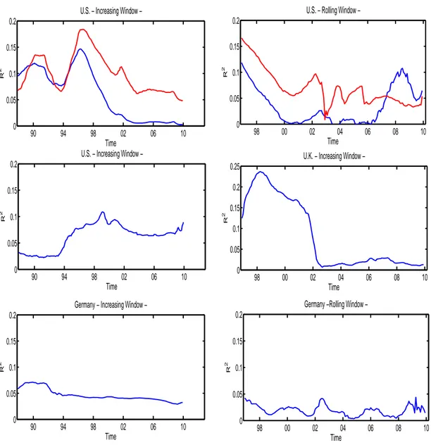
extend the analysis to different sample periods we notice from Figure2 that, regardless the fact to use

an increasing or a rolling window of observations in the estimations, we always detect positive values for

the ADP Pg.

Our factors contain useful information to forecast future inflation rates as well. The ADP Pπ is always

positive but with different amplitude across countries. We note a general reduction in the ADP Pπ when

we consider a five years maturity spectrum. However, this is not the case for U.S. and Japan yields when

we use the PST data set. Moreover, we notice that DP Pπt+h is equal to zero for 12 and 18 months ahead

forecasts in U.S., when a maturity spectrum from 1 to 9 years is considered. More precisely, in Japan we

find the best performances, both using a nine and five years maturity spectrum, with ADP Pπ of 11.2%

and 12.8% respectively, when the PST database is considered. Conversely, in U.K. the ADP Pπis of 3.6%

for a nine years maturity spectrum and only 1% when yields from one to five years are used. The ADP Pπ

is also (always) positive across different sample periods in all the countries considered, as highlighted by

Figure115_.

Tables12to14display that, regardless the database considered and for both the industrial production

growth and inflation rates, lower and upper bounds of the 90% confidence intervals for the R2 are higher

in predictive regressions using our factors than competing regressors in the literature.

To sum up the results presented above, we have empirically verified that our findings in Section 3.3

and3.4 are robust to a battery of robustness checks. In other words, considering different methods to

interpolate international yield curves or different sample periods do not prevent our extracted factors

outperform classical competitors in forecasting macroeconomic variables16_.

12_{We observe a general decrease in the DP P}

rx(n)_t+1 when a five maturity spectrum is considered with

Germany being the only exception.

13_{Results are available upon request from the author.}

14_{However, we observe a general reduction in the ADP P}

g when a five years maturity spectrum is

considered.

15_{Although the ADP P}

π is always positive in U.S., the amplitude depends upon the interpolation

technique used in the construction of the data.

16_{In Table 17we show that we reach similar conclusions when we use the data set kindly supplied by}

4

Conclusions

This paper documents the presence of relevant economic information hidden in the cross-section of ex-pected excess bond returns of four leading markets (U.S., U.K., Germany and Japan).

We estimate and select the preferred number of factors driving excess bond returns both using a clas-sical principal component approach and maximum likelihood criteria (AICb) and parameters significance within a linear Gaussian state-space approach.

We show that factors explaining only a small fraction of the variance of expected bond returns

are judged important when a Kalman-filter based maximum likelihood estimation is applied. More

importantly, these factors add a forecasting power over and above the information contained in classical predictors proposed by the literature, such as the return-forecasting factor and the yield curve factor [see

Ang and Piazzesi(2003),Diebold, Li, and Yue(2008),Cochrane and Piazzesi (2005) andCochrane and Piazzesi(2008)].

Our results are robust to battery of robustness checks making sure that our findings are not sample or country-dependent and do not rely on the interpolation technique used in the construction of international yield curves data.

Appendix

5

Model Estimation

U.S.

U.K.

GER

Japan

Marg.

Cum.

Marg.

Cum.

Marg.

Cum.

Marg.

Cum.

1

95.40

95.40

97.48

97.48

97.20

97.20

97.59

97.59

2

4.41

99.81

2.35

99.82

2.64

99.84

2.35

99.94

3

0.18

99.99

0.17

100.00

0.16

99.99

0.05

99.99

4

0.01

100.00

0.00

100.00

0.01

100.00

0.01

100.00

5

0.00

100.00

0.00

100.00

0.00

100.00

0.00

100.00

6

0.00

100.00

0.00

100.00

0.00

100.00

0.00

100.00

7

0.00

100.00

0.00

100.00

0.00

100.00

0.00

100.00

8

0.00

100.00

0.00

100.00

0.00

100.00

0.00

100.00

9

0.00

100.00

0.00

100.00

0.00

100.00

0.00

100.00

Table 1:

We report principal component analysis of the expected excess returns of each given country.

The first column lists the number of principal components, while the rest of the table is divided into four vertical blocks. Each of these blocks represents an individual country. The first and second columns of each block report marginal and cumulative percent variance explained for expected excess bond returns. We derive forward rates and calculate expected excess bond returns by using the international Treasury

yield curve database ofPegoraro, Siegel, and Tiozzo Pezzoli(2012). For any country, yields are observed

monthly from January 1, 1986 to December 31, 2009 (288 observations) and with residual maturities from 1 to 9 years. U.S. U.K. k Ξ L(bθM LE T ) AI C b k Ξ L(bθTM LE) AI C b 1 25 -928 1222 1 25 -1481 2234 2 36 1769 -4604 2 36 698 -2350 3 49 3462 -7514 3 49 2613 -5518 4 64 6135 -12658 4 64 2979 -6090 5 81 7756 -14800 5 81 3148 -6434 GER JAP k Ξ L(bθM LE T ) AI C b k Ξ L(bθTM LE) AI C b 1 25 -1243 1730 1 25 -1531 2076 2 36 1033 -2858 2 36 1128 -3098 3 49 3431 -7382 3 49 2615 -5918 4 64 4643 -9670 4 64 5145 -10798 5 81 6799 -10214 5 81 5783 -11932

Table 2:

For any given country and for any given number of latent factors k we provide the number of

parameters Ξ, the maximum value of the log-likelihood function (L(bθM LE

T )) and the associated bootstrap

variant of the Akaike Information Criteria ofCavanaugh and Shumway (1997). We derive forward rates

and calculate expected excess bond returns by using the international Treasury yield curve database of

Pegoraro, Siegel, and Tiozzo Pezzoli(2012). For any country, yields are observed monthly from January 1, 1986 to December 31, 2009 (288 observations) and with residual maturities from 1 to 9 years.

Country ΛB Φ 0,23∗∗ _0,12∗∗ _-0,04∗∗ _0,02∗∗ _0,00∗∗ _0,78∗∗ _{-0,07 0,06}∗∗ _{0,04 -0,08} U.S. (13,12) (13,05) (-10,58) (11,67) (14,15) (17,13) (-1,58) (2,25) (1,21) (-1,56) 0,46∗∗ _0,20∗∗ _-0,04∗∗ _0,00∗ _0,00∗∗ _{-0,05 0,79}∗∗ _-0,09∗∗ _{-0,02 0,04} (14,68) (13,85) (-16,37) (-1,78) (-12,55) (-0,21) (16,59) (-2,66) (-0,59) (0,54) 0,64∗∗ _0,22∗∗ _-0,01∗∗ _-0,02∗∗ _0,00∗∗ _{0,05 0,00 0,85}∗∗ _{-0,09 0,13}∗∗ (15,79) (13,14) (-2,90) (-14,05) (-15,18) (0,92) (-0,71) (20,99) (-1,55) (2,03) 0,78∗∗ _0,18∗∗ _0,02∗∗ _-0,01∗∗ _0,00∗∗ _{0,03 -0,04 -0,12}∗∗ _0,65∗∗ _0,09∗∗ (16,35) (11,34) (8,53) (-11,76) (15,38) (1,47) (-0,89) (-2,17) (11,90) (2,07) 0,88∗∗ _0,10∗∗ _0,03∗∗ _0,00∗∗ _0,00∗∗ _{0,07 0,01 0,06}∗ _{-0,09 0,58}∗∗ (15,84) (7,81) (15,66) (4,37) (16,10) (1,59) (0,26) (1,72) (-1,09) (9,43) 0,96∗∗ _{-0,01 0,03}∗∗ _0,01∗∗ _0,00∗∗ (14,19) (-0,74) (10,15) (11,31) (-14,26) 1,04∗∗ _-0,15∗∗ _0,01∗∗ _0,01∗∗ _0,00∗∗ (12,07) (-14,52) (2,92) (14,17) (-16,12) 1,12∗∗ _-0,30∗∗ _-0,03∗∗ _-0,01∗∗ _0,00∗∗ (10,13) (-15,31) (-12,39) (-10,03) (16,33) -0,48∗∗ _0,08∗∗ _0,09∗∗ _-0,01∗∗ _0,00∗∗ _0,51∗∗ _-0,15∗∗ _-0,20∗∗ _0,17∗∗ _0,18∗∗ U.K. (-22,03) (10,09) (20,87) (-17,43) (2,01) (8,15) (-3,34) (-3,56) (4,13) (2,57) -0,83∗∗ _0,16∗∗ _0,06∗∗ _{0,00 0,00}∗∗ _-0,23∗∗ _0,79∗∗ _-0,18∗∗ _{0,03 0,18}∗∗ (-22,42) (18,00) (20,11) (1,63) (3,46) (-4,35) (17,84) (-3,54) (0,55) (2,55) -1,10∗∗ _0,20∗∗ _0,02∗∗ _0,01∗∗ _{0,00 -0,30}∗∗ _-0,11∗ _0,60∗∗ _{0,09 0,24}∗∗ (-22,59) (21,47) (11,27) (17,18) (-1,56) (-5,06) (-1,95) (9,64) (1,50) (2,67) -1,32∗∗ _0,18∗∗ _-0,02∗∗ _0,00∗∗ _0,00∗∗ _0,13∗ _0,11∗∗ _0,10∗ _0,89∗∗ _-0,09∗ (-22,83) (21,08) (-12,08) (11,42) (-4,41) (1,64) (2,88) (1,70) (23,88) (-1,81) -1,51∗∗ _0,12∗∗ _-0,05∗∗ _0,00∗∗ _0,00∗∗ _0,36∗∗ _{0,13 0,36}∗∗ _{-0,07 0,73}∗∗ (-23,12) (17,72) (-20,89) (-2,07) (7,95) (2,55) (1,54) (2,69) (-0,94) (14,27) -1,65∗∗ _0,02∗∗ _-0,04∗∗ _-0,01∗∗ _0,00∗∗ (-23,23) (5,77) (-19,61) (-11,19) (-10,49) -1,81∗∗ _-0,13∗∗ _-0,02∗∗ _0,00∗∗ _0,01∗∗ (-23,08) (-21,18) (-15,26) (-4,16) (9,59) -1,94∗∗ _-0,31∗∗ _0,04∗∗ _0,01∗∗ _0,00∗∗ (-22,50) (-21,35) (15,86) (13,57) (-6,52) -0,27∗∗ _-0,12∗∗ _0,07∗∗ _-0,02∗∗ _0,00∗∗ _0,51∗∗ _-0,16∗∗ _0,15∗∗ _{-0,08 0,07}∗∗ GER (-15,49) (-11,90) (13,94) (-17,43) (14,49) (8,52) (-2,27) (4,59) (0,14) (3,10) -0,60∗∗ _-0,22∗∗ _0,07∗∗ _0,00∗ _0,00∗∗ _{-0,07 0,81}∗∗ _{0,02 -0,01}∗ _0,03 (-16,25) (-14,19) (14,66) (-1,85) (-17,00) (-1,11) (18,71) (0,72) (-1,69) (-0,84) -0,92∗∗ _-0,26∗∗ _0,03∗∗ _0,01∗∗ _0,00∗∗ _0,13∗∗ _{0,01 0,76}∗∗ _-0,14∗∗ _-0,03∗∗ (-16,52) (-14,25) (9,85) (17,01) (-13,73) (3,72) (0,26) (18,92) (-2,52) (-2,13) -1,20∗∗ _-0,23∗∗ _-0,02∗∗ _0,01∗∗ _0,00∗∗ _{-0,02 -0,04 -0,05 0,56}∗∗ _-0,21∗∗ (-16,48) (-12,89) (-7,71) (15,55) (16,73) (0,78) (-1,13) (-1,32) (8,48) (-4,76) -1,45∗∗ _-0,15∗∗ _-0,05∗∗ _0,00∗∗ _0,00∗∗ _{0,07 -0,08}∗∗ _{0,00 -0,18}∗ _0,67∗∗ (-16,09) (-10,32) (-14,24) (-4,18) (17,06) (1,25) (-2,00) (-0,51) (-1,88) (20,65) -1,68∗∗ _-0,02∗∗ _-0,05∗∗ _-0,01∗∗ _0,00∗∗ (-15,28) (-3,71) (-14,26) (-16,66) (-13,38) -1,89∗∗ _0,14∗∗ _-0,01∗∗ _-0,01∗∗ _0,00∗∗ (-14,15) (14,49) (-8,27) (-15,83) (-16,70) -2,10∗∗ _0,32∗∗ _0,06∗∗ _0,01∗∗ _0,00∗∗ (-12,88) (13,69) (13,46) (16,19) (15,58) 0,37∗∗ _0,12∗∗ _-0,03∗∗ _0,03∗∗ _0,00∗∗ _0,70∗∗ _0,09∗∗ _0,19∗∗ _-0,16∗∗ _0,08∗∗ J AP (13,58) (12,23) (-7,55) (13,84) (-14,44) (13,02) (2,50) (4,10) (-3,03) (3,63) 0,76∗∗ _0,22∗∗ _-0,04∗∗ _0,01∗∗ _0,00∗∗ _{-0,02 0,86}∗∗ _{0,00 0,03 0,00} (13,48) (13,16) (-12,45) (10,86) (14,28) (0,41) (23,85) (-1,28) (0,58) (-1,01) 1,09∗∗ _0,27∗∗ _-0,03∗∗ _-0,01∗∗ _0,00∗∗ _0,13∗∗ _{0,04 0,78}∗∗ _{0,01 -0,07}∗∗ (13,58) (13,30) (-12,15) (-8,83) (13,66) (3,54) (0,38) (14,58) (0,71) (-2,60) 1,36∗∗ _0,25∗∗ _{0,00 -0,01}∗∗ _0,00∗∗ _-0,24∗∗ _0,10∗∗ _0,13∗∗ _0,74∗∗ _0,07∗∗ (13,78) (12,69) (-0,50) (-14,15) (-13,92) (-3,94) (2,43) (3,00) (16,27) (2,58) 1,58∗∗ _0,17∗∗ _0,03∗∗ _0,00∗∗ _0,00∗∗ _{0,00 0,02 -0,08 0,03 0,94}∗∗ (13,98) (10,61) (12,43) (-7,57) (-14,12) (0,24) (0,12) (-1,49) (0,36) (35,39) 1,76∗∗ _0,02∗∗ _0,04∗∗ _0,01∗∗ _0,00∗∗ (13,99) (2,53) (13,83) (7,21) (12,06) 1,90∗∗ _-0,17∗∗ _0,02∗∗ _0,01∗∗ _0,00∗∗ (13,60) (-13,47) (11,03) (11,09) (13,39) 2,00∗∗ _-0,41∗∗ _-0,05∗∗ _-0,01∗∗ _0,00∗∗ (12,63) (-13,36) (-13,53) (-7,27) (-13,18)

Table 3:

We report the maximum likelihood estimates of ΛB and Φ parameters and the associated

bootstrap t-students (in parenthesis) for state-space models in (17) for U.S., U.K., GER and JAP. We

use Nonparametric Monte Carlo bootstrap [seeStoffer and Wall(1991) andPolitis and Romano(1994);

the optimal block sizes are chosen following Politis and White (2004) and Patton, Politis, and White

6

F

or

eca

sti

ng

E

xce

ss

b

o

nd

Ret

urns

n xU.S .,t R 2 f (n ) U.S .,t − y (1) U.S .,t R 2 LU.S .,t SU.S.,t CU.S .,t R 2 n xGE R ,t R 2 f (n ) GE R ,t − y (1) GE R ,t R 2 LGER ,t SGE R ,t CGE R ,t R 2 rx (n ) U.S .,t +1 2 0,23 0,05 0,15 0,00 4,43 -8, 91 -32, 91 0,02 rx (n ) GE R ,t+1 2 0,15 ∗ 0,06 0,19 0,00 0,72 5,94 -52, 80 0,00 (1, 43) {0, 00; 0,20 } (0, 34) {0, 00; 0,16 } (1, 06) (-0, 35) (-0, 25) {0, 01; 0,32 } (1, 68) {0, 00; 0,21 } (0, 41) {0, 00; 0,14 } (0, 17) (0, 24) (-0, 74) {0, 00; 0,27 } 3 0,50 ∗ 0,06 0,30 0,01 6,71 -29, 55 -135, 69 0,03 3 0,41 ∗∗ 0,11 0,37 0,01 2,42 30, 46 -179, 00 0,03 (1, 66) {0, 00; 0,23 } (0, 60) {0, 00; 0,17 } (0, 91) (-0, 62) (-0, 55) {0, 01; 0,28 } (2, 46) {0, 01; 0,28 } (0, 73) {0, 00; 0,17 } (0, 29) (0, 67) (-1, 16) {0, 01; 0,31 } 4 0,75 ∗ 0,08 0,39 0,01 7,94 -54, 35 -240, 01 0,04 4 0,68 ∗∗ 0,15 0,48 0,02 4,08 62, 27 -295, 87 0,05 (1, 79) {0, 00; 0,23 } (0, 74) {0, 00; 0,15 } (0, 82) (-0, 84) (-0, 70) {0, 01; 0,29 } (3, 06) {0, 03; 0,33 } (0, 87) {0, 00; 0,19 } (0, 34) (1, 01) (-1, 25) {0, 02; 0,35 } 5 0,96 ∗ 0,08 0,47 0,01 8,85 -79, 94 -323, 14 0,04 5 0,93 ∗∗ 0,18 0,58 0,03 5,21 97, 11 -377, 17 0,07 (1, 88) {0, 00; 0,23 } (0, 84) {0, 00; 0,14 } (0, 78) (-1, 03) (-0, 77) {0, 01; 0,28 } (3, 55) {0, 06; 0,36 } (0, 98) {0, 00; 0,21 } (0, 34) (1, 32) (-1, 20) {0, 02; 0,38 } 6 1,14 ∗∗ 0,08 0,54 0,02 9,78 -105, 33 -384, 61 0,05 6 1,16 ∗∗ 0,21 0,69 0,03 5,64 133, 48 -418, 95 0,09 (1, 96) {0, 00; 0,24 } (0, 94) {0, 00; 0,11 } (0, 77) (-1, 19) (-0, 80) {0, 01; 0,27 } (3, 95) {0, 07; 0,38 } (1, 08) {0, 00; 0,21 } (0, 32) (1, 59) (-1, 09) {0, 03; 0,37 } 7 1,31 ∗∗ 0,09 0,62 0,02 10, 81 -130, 44 -429, 91 0,06 7 1,37 ∗∗ 0,22 0,82 0,04 5,34 170, 83 ∗ -424, 51 0,10 (2, 05) {0, 02; 0,18 } (1, 03) {0, 00; 0,15 } (0, 78) (-1, 34) (-0, 81) {0, 01; 0,24 } (4, 29) {0, 07; 0,40 } (1, 21) {0, 00; 0,22 } (0, 27) (1, 84) (-0, 96) {0, 03; 0,39 } 8 1,48 ∗∗ 0,09 0,71 0,02 11, 95 -155, 35 -464, 44 0,06 8 1,56 ∗∗ 0,23 0,98 0,05 4,38 208, 98 ∗∗ -398, 90 0,11 (2, 14) {0, 01; 0,23 } (1, 12) {0, 00; 0,15 } (0, 79) (-1, 47) (-0, 80) {0, 01; 0,22 } (4, 57) {0, 09; 0,42 } (1, 36) {0, 00; 0,23 } (0, 20) (2, 08) (-0, 80) {0, 03; 0,39 } 9 1,64 ∗∗ 0,09 0,80 0,02 13, 17 -180, 18 -492, 12 0,07 9 1,74 ∗∗ 0,24 1,17 0,07 2,81 247, 79 ∗∗ -346, 93 0,12 (2, 25) {0, 01; 0,22 } (1, 20) {0, 00; 0,16 } (0, 81) (-1, 59) (-0, 78) {0, 02; 0,27 } (4, 82) {0, 10; 0,42 } (1, 53) {0, 00; 0,25 } (0, 12) (2, 29) (-0, 64) {0, 03; 0,39 } n xU.K .,t R 2 f n U.K .,t − y 1 U.K .,t R 2 LU.K .,t SU.K .,t CU.K .,t R 2 n xJAP ,t R 2 f n JAP ,t − y 1 JAP ,t R 2 LJAP ,t SJAP ,t CJAP ,t R 2 rx (n ) U.K .,t +1 2 0,35 ∗∗ 0,29 0,50 ∗ 0,06 -0, 80 -22, 58 -206,48 ∗∗ 0,11 rx (n ) JAP ,t+1 2 0,26 ∗∗ 0,52 1,50 ∗∗ 0,19 3,31 -53, 78 ∗∗ 302, 21 ∗∗ 0,43 (4, 00) {0, 14; 0,49 } (1, 77) {0, 00; 0,27 } (-0, 17) (-1, 20) (-2,09) {0, 04; 0,38 } (7, 11) {0, 38; 0,72 } (2, 14) {0, 04; 0,49 } (1, 15) (-2, 32) (5, 65) {0, 27; 0,72 } 3 0,62 ∗∗ 0,29 0,58 0,05 1,30 -37, 90 -387, 88 ∗∗ 0,12 3 0,55 ∗∗ 0,57 1,78 ∗∗ 0,25 6,59 -129, 03 ∗∗ 616, 61 ∗∗ 0,48 (4, 29) {0, 16; 0,44 } (1, 64) {0, 00; 0,23 } (0, 17) (-1, 09) (-2, 29) {0, 05; 0,37 } (8, 13) {0, 42; 0,75 } (2, 57) {0, 07; 0,54 } (1, 19) (-2, 90) (5, 90) {0, 32; 0,74 } 4 0,84 ∗∗ 0,29 0,61 0,04 3,95 -55, 06 -524, 99 ∗∗ 0,13 4 0,81 ∗∗ 0,59 1,84 ∗∗ 0,24 8,49 -207, 24 ∗∗ 859, 35 ∗∗ 0,48 (4, 60) {0, 15; 0,45 } (1, 36) {0, 00; 0,17 } (0, 39) (-1, 11) (-2, 41) {0, 04; 0,35 } (8, 62) {0, 45; 0,75 } (2, 51) {0, 06; 0,51 } (1, 09) (-3, 29) (5, 82) {0, 33; 0,73 } 5 1,01 ∗∗ 0,28 0,60 0,03 6,28 -76, 45 -608, 37 ∗∗ 0,13 5 1,02 ∗∗ 0,58 1,88 ∗∗ 0,21 9,41 -281, 74 ∗∗ 1011, 25 ∗∗ 0,47 (4, 78) {0, 14; 0,45 } (1, 13) {0, 00; 0,13 } (0, 52) (-1, 19) (-2, 39) {0, 04; 0,36 } (8, 61) {0, 44; 0,74 } (2, 29) {0, 05; 0,46 } (0, 97) (-3, 54) (5, 52) {0, 32; 0,71 } 6 1,15 ∗∗ 0,27 0,63 0,02 8,17 -101, 75 -644, 38 ∗∗ 0,12 6 1,19 ∗∗ 0,57 1,89 ∗∗ 0,17 9,86 -350, 95 ∗∗ 1073, 48 ∗∗ 0,45 (4, 83) {0, 13; 0,44 } (1, 03) {0, 00; 0,13 } (0, 59) (-1, 30) (-2, 28) {0, 04; 0,37 } (8, 26) {0, 49; 0,65 } (2, 03) {0, 03; 0,41 } (0, 87) (-3, 68) (5, 06) {0, 29; 0,69 } 7 1,26 ∗∗ 0,25 0,68 0,02 9,47 -129, 29 -636, 41 ∗∗ 0,12 7 1,32 ∗∗ 0,54 1,83 ∗ 0,13 10, 18 -414, 74 ∗∗ 1051, 85 ∗∗ 0,42 (4, 72) {0, 11; 0,43 } (1, 00) {0, 00; 0,12 } (0, 61) (-1, 40) (-2, 10) {0, 03; 0,35 } (7, 69) {0, 39; 0,70 } (1, 77) {0, 01; 0,35 } (0, 80) (-3, 78) (4, 46) {0, 28; 0,65 } 8 1,35 ∗∗ 0,23 0,80 0,03 10, 14 -158, 77 -595,26 ∗ 0,11 8 1,41 ∗∗ 0,50 1,71 0,10 10, 58 -473, 05 ∗∗ 951, 41 ∗∗ 0,40 (4, 52) {0, 09; 0,41 } (1, 10) {0, 00; 0,14 } (0, 60) (-1, 50) (-1, 86) {0, 03; 0,34 } (6, 94) {0, 33; 0,69 } (1, 54) {0, 00; 0,31 } (0, 75) (-3, 84) (3, 71) {0, 24; 0,61 } 9 1,42 ∗∗ 0,21 0,95 0,04 10, 17 -189, 48 -527, 15 0,10 9 1,45 ∗∗ 0,45 1,53 0,08 11, 17 -525, 58 ∗∗ 775, 14 ∗∗ 0,37 (4, 24) {0, 09; 0,39 } (1, 19) {0, 00; 0,16 } (0, 55) (-1, 58) (-1, 58) {0, 03; 0,34 } (5, 99) {0, 29; 0,64 } (1, 39) {0, 00; 0,26 } (0, 74) (-3, 90) (2, 74) {0, 23; 0,56 }

T

a

b

le

4:

W e re p or t the res ul ts of fore cas tin g re gre ss ion s of U .S ., U .K ., GE R an d J AP ex cess b on d re tur n s (r xt+1 ) u si n g as re gre ssor s th e CP fact or , th e for w ar d-s p ot sp re ad an d th e y ie ld cu rv e fact or s (Le v el , Sl op e and Cu rv atu re) .W e re p or t est imat es for p aram et er s (m u lt ip lie d b y 10 2; con st an t ter ms , in cl u de d in th e regr es si ons , ar e om it te d from th e tab le ) alon g wi th t-s tud en ts (i n p are n th es is) bas ed on New ey an d W est ( 1987 ) st and ar d er ror s con si d er ing cond iti on al h et er osce das tic it y an d ser ial cor rel at ion u p to 12 lags . O ne and tw o ast er isk s d en ot e st at ist ical ly si gni fi can ce at 10% an d 5% lev el s, res p ect iv el y. W e al so re p or t adj u st ed R 2 wi th 90% b o ot st rap p ed confi d en ce in ter v als in cur ly br ac k et s. W e us e mon th ly d at a (P S T d at abas e) for a sam pl e p eri o d st ar tin g from J an u ary 1, 1986 ti ll D ece m b er 31, 2009 (288 ob se rv at ion s) and wi th re si d ual mat u ri ti es fr om 1 to 9 y ears .

n b (n ) U .S ., 1 b (n ) U .S ., 2 b (n ) U .S ., 3 b (n ) U .S ., 4 b (n ) U .S ., 5 R 2 n b (n ) GE R ,1 b (n ) GE R ,2 b (n ) GE R ,3 b (n ) GE R ,4 b (n ) GE R ,5 R 2 r x (n ) U .S .,t +1 2 -0, 23 ∗∗ -0, 12 0, 04 0, 02 0, 00 0,07 r x (n ) GE R ,t +1 2 -0, 27 ∗∗ 0, 12 0, 07 0,02 0, 00 0, 07 (-2, 07) (-1, 23) (0, 55) (0, 26) (-0, 01) { 0, 04; 0,31 } (-2, 82) (1, 42) (1, 50) (0,38) (0, 06) { 0, 06; 0,31 } 3 -0, 46 ∗∗ -0, 20 0, 04 0, 00 0, 00 0,07 3 -0, 60 ∗∗ 0, 22 0, 07 0,00 0, 00 0, 12 (-2, 20) (-1, 09) (0, 25) (-0, 0 1) (0, 01) { 0, 04; 0,31 } (-3, 34) (1, 46) (0, 68) (0,01) (-0, 03) { 0, 08; 0,36 } 4 -0, 64 ∗∗ -0, 22 0, 01 -0, 02 0, 00 0, 07 4 -0, 92 ∗∗ 0, 26 0, 03 -0, 01 0, 00 0, 15 (-2, 21) (-0, 87) (0, 05) (-0, 0 7) (0, 00) { 0, 04; 0,30 } (-3, 69) (1, 29) (0, 17) (-0, 08) (-0, 01) { 0, 10; 0,39 } 5 -0, 78 ∗∗ -0, 18 -0, 02 -0,01 0, 00 0, 07 5 -1, 20 ∗∗ 0, 23 -0,02 -0, 01 0,00 0, 18 (-2, 16) (-0, 59) (-0, 06) (-0, 04) (0,00) { 0, 04; 0,29 } (-3, 91) (0, 97) (-0, 09) (-0, 05) (0, 01) { 0, 12; 0,42 } 6 -0, 88 ∗∗ -0, 10 -0, 03 0, 00 0, 00 0, 07 6 -1, 45 ∗∗ 0, 15 -0,05 0, 00 0, 00 0, 20 (-2, 11) (-0, 29) (-0, 10) (0, 01) (0, 00) { 0, 03; 0,28 } (-4, 04) (0, 55) (-0, 17) (0, 01) (0, 01) { 0, 12; 0,44 } 7 -0, 96 ∗∗ 0, 01 -0, 03 0, 01 0, 00 0,07 7 -1, 68 ∗∗ 0, 02 -0,05 0, 01 0, 00 0, 21 (-2, 07) (0, 02) (-0, 08) (0, 04) (0, 00) { 0, 03; 0,24 } (-4, 12) (0, 08) (-0, 14) (0, 04) (0, 00) { 0, 12; 0,45 } 8 -1, 04 ∗∗ 0, 15 -0, 01 0, 01 0, 00 0,08 8 -1, 89 ∗∗ -0, 14 -0, 01 0, 01 0,00 0, 23 (-2, 04) (0, 32) (-0, 02) (0, 03) (0, 00) { 0, 03; 0,27 } (-4, 17) (-0,41) (-0, 04) (0, 03) (-0,01) { 0, 13; 0,47 } 9 -1, 12 ∗∗ 0, 30 0, 03 -0, 01 0, 00 0,08 9 -2, 10 ∗∗ -0, 32 0,06 -0, 01 0,00 0, 24 (-2, 03) (0, 61) (0, 08) (-0, 03) (0, 00) { 0, 03; 0,29 } (-4, 23) (-0,89) (0, 13) (-0, 03) (0, 01) { 0, 14; 0,48 } n b (n ) U .K ., 1 b (n ) U .K ., 2 b (n ) U .K ., 3 b (n ) U .K ., 4 b (n ) U .K ., 5 R 2 n b (n ) J AP ,1 b (n ) J AP ,2 b (n ) J AP ,3 b (n ) J AP ,4 b (n ) J AP ,5 R 2 r x (n ) U .K .,t +1 2 -0, 48 ∗∗ -0, 08 -0, 09 0, 01 0, 00 0, 32 r x (n ) J AP ,t +1 2 -0, 37 ∗∗ 0, 12 ∗∗ 0, 03 0, 03 0, 00 0,58 (-4, 22) (-0, 87) (-0, 84) (0, 14) (0, 02) { 0, 22; 0,48 } (-5, 87) (2, 58) (0, 65) (1,00) (-0, 07) { 0, 49; 0,72 } 3 -0, 83 ∗∗ -0, 16 -0, 06 0, 00 0, 00 0, 30 3 -0, 76 ∗∗ 0, 22 ∗∗ 0, 04 0, 01 0, 00 0,61 (-4, 55) (-1, 08) (-0, 35) (-0, 03) (0,01) { 0, 18; 0,49 } (-6, 08) (2, 48) (0, 44) (0,17) (0, 01) { 0, 49; 0,81 } 4 -1, 10 ∗∗ -0, 20 -0, 02 -0,01 -0, 01 0,29 4 -1, 09 ∗∗ 0, 27 ∗∗ 0, 03 -0,01 0, 00 0, 61 (-4, 75) (-1, 11) (-0, 09) (-0, 07) (-0, 04) { 0, 18; 0,50 } (-6, 12) (2, 03) (0, 22) (-0, 09) (-0, 01) { 0, 49; 0,79 } 5 -1, 32 ∗∗ -0, 19 0, 01 -0, 02 -0, 01 0, 28 5 -1, 36 ∗∗ 0, 25 0, 00 -0, 01 0, 00 0, 59 (-4, 76) (-0, 90) (0, 03) (-0, 0 6) (-0,07) { 0, 18; 0,49 } (-6, 02) (1, 42) (0, 02) (-0, 10) (-0, 02) { 0, 46; 0,77 } 6 -1, 50 ∗∗ -0, 12 0, 03 -0, 01 -0, 01 0, 26 6 -1, 59 ∗∗ 0, 17 -0,03 0, 00 0, 00 0, 56 (-4, 64) (-0, 53) (0, 08) (-0, 0 4) (-0,07) { 0, 16; 0,49 } (-5, 86) (0, 76) (-0, 11) (-0, 02) (-0,01) { 0, 45; 0,74 } 7 -1, 65 ∗∗ -0, 02 0, 01 -0, 01 -0, 03 0, 24 7 -1, 76 ∗∗ 0, 02 -0,04 0, 01 0, 00 0, 53 (-4, 39) (-0, 10) (0, 02) (-0, 0 2) (-0,11) { 0, 15; 0,46 } (-5, 66) (0, 09) (-0, 15) (0, 05) (0, 00) { 0, 42; 0,71 } 8 -1, 80 ∗∗ 0, 13 -0, 01 -0, 02 -0, 02 0, 23 8 -1, 90 ∗∗ -0, 17 -0, 02 0, 01 0,00 0, 50 (-4, 23) (0, 45) (-0, 01) (-0, 0 4) (-0,07) { 0, 13; 0,45 } (-5, 46) (-0,57) (-0, 07) (0, 06) (0, 00) { 0, 38; 0,70 } 9 -1, 94 ∗∗ 0, 30 -0, 07 -0, 03 -0, 03 0, 22 9 -2, 00 ∗∗ -0, 41 0,05 -0, 01 0,00 0, 47 (-4, 05) (0, 98) (-0, 14) (-0, 0 6) (-0,11) { 0, 13; 0,42 } (-5, 26) (-1,22) (0, 13) (-0, 03) (-0,01) { 0, 35; 0,67 }

T

a

b

le

5:

W e re p or t th e re su lt s of fore cas ti n g regr es si on s of U .S ., U .K ., GE R an d J AP ex cess b ond ret u rns (r xt+1 ) u si n g as re gr ess ors th e smo ot h ed fact or s ex trac ted from th e fiv e fact or s st at e-s pac e mo d el .W e rep or t est imat es for p aram et er s (con st an t te rm s, in cl u de d in th e regr es si ons , ar e omi tt ed from th e tab le) al ong wi th t-st u de n ts (in p are n th es is ) bas ed on Ne w ey and W es t ( 1987 ) stan d ard er rors con si d er ing con d it ion al he te rosce das ti ci ty an d se rial cor rel at ion up to 12 lags . O ne an d tw o ast eri sk s d en ot e st at ist ical ly si g n ifi can ce at 10% and 5% lev els , res p ect iv el y. W e al so re p or t ad jus ted R 2 wi th 90% b o ot st rapp ed confi d en ce in ter v al s in cur ly b rac k et s. W e us e m on th ly dat a (P S T d at abas e) for a samp le p er io d st ar tin g fr om J an uar y 1, 1986 ti ll D ecem b er 31, 2009 (288 ob se rv at ions ) and wi th re si du al mat u ri ti es fr om 1 to 9 y ear s.