lamsade
LAMSADE
Laboratoire d’Analyse et Modélisation de Systèmes pour
l’Aide à la Décision
UMR 7243
JUILLET 2016CAHIER DU
375
A DSS approach for heterogeneous parallel machines scheduling with due windows, processor-&-sequence dependent setup and proximate supply chain constraints
Ahlam Azzaouri, Imane Essaadi, Pierre Fénies, Fréderic Fontane, Vincent Giard
A DSS approach for heterogeneous parallel machines scheduling with due
windows, processor-&-sequence-dependent setup and proximate supply
chain constraints
Ahlam Azzamouri
a, Imane Essaadi
a, Pierre Fénies
b,a, Frédéric Fontane
a,c,
Vincent Giard
d,aa) EMINES School of Industrial Management, University Mohammed VI, Ben Guerir, Morroco
b) University Paris Ouest Nanterre La Défense, Nanterre, France c) ParisTech-Mines, Paris, France
d) LAMSADE, PSL-University Paris-Dauphine, Paris, France
This paper describes the basis of a Decision Support System (DSS) designed to support scheduling for a fertilizer production plant made up of several parallel lines of heterogeneous characteristics, with setup time depending on sequence and lines, and taking into account non-availability constraints; it also considers the primary impacts of schedule upstream and downstream of the supply chain which integrates the plant. Our DSS uses an original MILP scheduling formulation whose implementation, through an Algebraic Modeling Languages (AML), facilitates interaction with the scheduler to formulate an instantiated problem whose optimal solution is acceptable.
Keywords: Decision Support System, Optimization, Scheduling, Heterogeneous
Parallel Processors, Sequence Dependent Setup, Non-Availability Constraints. Supply chain
Introduction
OCP SA (http://www.ocpgroup.ma/fr) accounts for one third of world phosphate exports across product segments. The Jorf fertilizer production plant, located near the sea at the end of the Northern axis of OCP’s supply chain (SC), is the Moroccan group’s largest plant. It produces some twenty one fertilizer references at 7 parallel lines(3 “107” identical lines and 4 “07” identical lines); 7 out of 21 references may only be produced at a single type of line, which yields 35 routings. Fertilizer demand is seasonal and produced to order, with shipping performed by boat at the harbour located near the fertilizer plant. The subject of our paper is the issue of scheduling a set of orders for the production lines starting from a date, without
interfering with orders in process at that date. Each order is characterized by a fertilizer reference to be manufactured, a tonnage and a time window during which production must be completed. The schedule must factor in production stoppage required by preventive maintenance operations, and such stoppage has no impact on ongoing production time. Order fulfillment time varies from line to line, in particular due to their different technical features and due to production rate modulation options. The schedule must also factor in substantial cleaning operation time between two batches of production of different quality on the same line. Such line preparation lead time depends on the line itself and on the previously produced reference.
The proposed schedule has immediate upstream and downstream consequences that may make it unfeasible due to pump priming issues (upstream) or finished product inventory saturation (downstream):
• Fertilizer manufacturing requires, among other inputs, sulfuric acid and phosphoric acid, the latter using sulfuric acid as a component. Jorf’s site SC comprises production units for both acids. Moreover, the phosphoric acid that it produces is also exported and shipped and both acids may be used by the Joint Ventures (JV) also operating at Jorf. An analysis of the fertilizer BOM’s reveals a strong dispersion on the consumption rate for these inputs (for example, production of one tonne of NPK 14-23-14 1B fertilizer requires nearly 7 times more pure phosphoric acid than one tonne of MAP Std (11-52) fertilizer). This means that the adopted scheduling has a strong impact on consumption rate for these acids and that the schedule is only workable if it does not deplete inventory for these raw materials.
• The manufactured fertilizers are carried by conveyer belts out of the six storage areas. The storage areas are dedicated to the fertilizer references belonging to a particular family. Area capacity varies depending on the number of stored references, as any mixing of fertilizers is highly hazardous. The allocation of such areas to product families changes over time and
several areas may be dedicated to a single family. Stored fertilizers are moved on conveyer belts to be loaded on the boats to fulfill orders, most of which concern a single reference. Loading takes a few days as per a schedule (that may be altered due to weather conditions). Residual storage capacity for a fertilizer reference therefore, varies over time. The chosen schedule determines fertilizer inventory build up and will not be workable if inventory build up is not matched by storage capacity.
Production stoppage risk due to pump priming issues (upstream) and/or saturated storage (downstream) serves to place the scheduling problem in the wider framework of SC management for the relevant fertilizer plant.
The coherence of operational and tactical decisions taken by the different entities of a SC is extremely difficult to guarantee, as a result of which substantial loss of efficiency and effectiveness may be sustained. The reasons are easy enough to explain. One is substantial decision-making autonomy, supported by local performance assessment systems that hampers multiple entity collaboration and promotes a local management focus. Another is the fact that centralized decision-making to eliminate causes of poor performances due to organizational factors is practically impossible to implement in a SC due to modelling complexity and calculation complexity. SC management generally involves a mix of local decisions and regulatory decisions taken at a higher level, upon detection (often too late) of the fact that the supply chain is no longer under control. Where the variety of products moving along the SC is not too great, one may restrict regulatory decisions through judicious recourse to buffer inventory. This solution, while enhancing decisional decoupling though it does not guarantee it, involves a loss of efficiency. An alternative consists in setting up decisional patterns that sharply reduce local decision-making, through upper-level regulation based on constraint trade-offs between the different links of the SC and a posteriori regulation for remedial measures to substantial disruptions. In this context, the Decision Support Systems (DSS) appear a useful
approach to improve the relevance of decisions taken in a SC. This is precisely the option explored in this paper with a restricted scope for a fertilizer plant scheduling exercise that is limited to the direct upstream (to avoid pump priming issues) and downstream constraints (to avoid saturation).
The bases for DSS were laid by Gorry and Scott Morton (1971) and transformed into a proper system by Keen and Scott Morton (1978). IS/IT development of course immensely increased the potential of DSS (Shim et al., 2002; Eomi & Kim, 2006; Bhargava et al. 2007…) without altering its rationale. Basically DSSs comprise: 1) an interface to formally express a complex issue that is partially structured to define a structured problem; 2) one or multiple modules to solve the structured problem, usually based on optimization or simulation models (Power and Sharda, 2007); 3) an interface capable of exploring all the consequences of a solution obtained and of either adjusting it marginally or of validating it; 4) if none of these solutions is acceptable, the DSS then is used to define a new structured problem using the feedback from prior formulations that failed to deliver a satisfactory solution.
The DSS concept used to solve the scheduling issue of the Jorf fertilizer plant (Azzamouri
et al., 2016) is set forth under section IV. The structured problem that lies at the heart of module
2 of the DSS corresponds to the problem of a locally defined schedule that i) does not factor in the upstream or downstream constraints (model 1) or ii) factors these constraints in (model 2), although the operational value of the latter formulation is limited for numerical reasons. An analysis of literature (section II) reveals that none of the proposed formulations reflects the full complexity of the problem at hand. Both models are described under section III and their use is illustrated by an example. After this presentation of the DSSS (section IV), we conclude our paper with a few comments on its implementation
Literature review
The fact that the fertilizer production process is a continuous one does not mean that the scheduling problem is not of the discrete type since order production time at a given line is predetermined by the line itself and by the previously produced reference (which may require a preparation lead time prior to launching production). Note that additionally the different stages of a continuous manufacturing process are not relevant for scheduling purposes as these are implicitly defined at “line-end”. Each line may be viewed as a standalone processor and the processors are heterogenous since the fulfillment time of orders is not the same for all processors. The scheduling problem consists in allocating orders to processors and in sequencing the different orders allocated to each line, while taken into account all the above listed considerations.
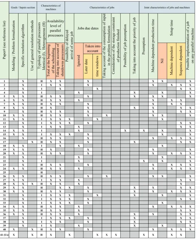
We therefore looked at the literature dealing with the scheduling of orders for heterogenous processors. We have analyzed 40 recent articles published in the best journals, by using an analysis grid organized along five axes. This analysis is summarized in table 1 whose last line shows the characteristics retained simultaneously in our approach.
• Characteristics of processors. The production system is made of parallel processors. They can be identical, if any job can be processed by any machine with the same production time, or heterogeneous, in the opposite case. The availability of those processors may be permanent or not (preventive maintenance…); at the beginning of the schedule, all processors may be available or not (orders in progress).
• Characteristics of jobs. Jobs can be all available to be launched when schedule starts, or not (progressive arrivals). In both cases, the characteristics of all jobs are known. Due
dates constraints may have to be met (through upper bounds or time windows) or not
considered. Preemption may be authorized or not. In some papers, automatic splitting of the ordered quantity is integrated. The consequences of the solution, upstream and
downstream of the supply chain, may imply the introduction of additional constraints in the problem definition
• Characteristics linked simultaneously with jobs and processors. Heterogeneity implies differences of production times and the impossibility, for some processors, to treat some productions. Setup times, where applicable, may depend on the sequence and/or the processor.
• Optimization criteria. Few optimization criteria use an economic point of view; most relate to efficiency (makespan…). Due to lack of space, this aspect is not considered here. • Paper’s aims. A scientific paper is written with a specific aim. Three categories of targets can be identified: the numerically-oriented ones (new algorithm to solve a specific class of problems, analysis of the limits of existing algorithm…); the model- oriented ones (new formulation of a complex problem, sometimes preceded by a representative case study or followed by a small academic case study used to illustrate problem formalization); another category, not encountered in the surveyed papers, is description-oriented, devoted to explanation of complex, real situations.
Table 1. Main characteristics of the analysed papers
Definition of scheduling problem
Two models for MILP scheduling issues are proposed (§III.1) and their use is illustrated by a limited numerical example (§III.2). But the combinatory explosion of model 2 versus model
1 X H X X X X X X 2 X I X X X X X X X 3 X I X X X X 4 X I X X X X 5 X X H X X X X X X X 6 X X H X X X X X X 7 X X H X X X X X X 8 X X H X X X X X X 9 X H X X X X X X 10 X X H X X X X X X X 11 X X I X X X X X 12 X I X X X X X X 13 X I X X X X X 14 X X I X X X X X 15 X X I X X X X X X 16 X H X X X X X X X 17 X H X X X X X X 18 X X I X X X 19 X X H X X X X 20 X X H X X X X X X X 21 X I X X X 22 X I X X X X 23 X H X X X X X X X 24 X X H X X X X X X X 25 H 26 X X H X X X X X X X 27 X X I X X X X X 28 X X X H X X X X 29 X X H X X X X X X X 30 X X H X X X X X X X X 31 X I X X X X X X X 32 X I X X X X X X 33 X I X X X X X 34 X X H X X X X X X X 35 X X H X X X X X 36 X X H X X X X X X X 37 X I X X X X X X X 38 X I X X X X X X 39 X I X X X X X 40 X X H X X X X X X X 41 (Us) X X H X X X X X X X X X M ac hi ne de pe nde nt pr oduc tion t im e Pa pe r# (s ee re fe re nc e l ist )
Goals / Inputs section Characteristics of machines Characteristics of jobs Joint characteristics of jobs and machines
Se tu p time Po ss ib le imp le me nta tio n o f a jo b on a ny pa ra lle l m ac hi ne Tot al a t t he be gi nni ng of the sc he dul ing Ta ki ng i nt o a cc ount of shut dow ns pr oc es sor s Ignor ed Taken into account Ni l M ac hi ne de pe nde nt Se que nc e de pe nde nt La te r d at e Pos sibi lit y of de la ye d a rr iva l of som e j ob
Jobs due dates
Pr ee mp tio n time w in do w s Ta ki ng a cc ount of the c ons um pt ion of input s in t he pr obl em for m ul at ion Cons ide ra tion of the st or age c ons tra int of pr oduc tion f ini she d Pos sibi lit y of job pr ee m pt ion Ta ki ng i nt o a cc ount the pr ior ity of job M od elin g / P ro ble m f or ma liz atio n Spe ci fic re sol ut ion a lgor ithm U se of ge ne ra l r es ol ut ion m et hods Typol ogy of pa ra lle l pr oc es sor s Ide nt ic al (I ), H et er oge ne ous (H ) Availability level of parallel processors
1 leads one to prefer model 1 in the DSS in order to have acceptable calculation time. We shall briefly review the definition of the economic valuation system for the decisions to be made, an aspect all too often left aside by operational research experts (§III.3)
III.1 Models of the scheduling problem
Two models for the scheduling problem have been proposed (Giard et al., 2015; Azzamouri
et al., 2016). Model 1 is based on local reasoning and ignores possible unavailability of raw
materials (upstream of the SC) and any saturation of finished product inventories (downstream of the SC). Model 2 takes these constraints explicitly into account.
The two models share multiple features, thus justifying joint presentation. The model parameters combine ranges and BOM information with information stemming from the orders to be fulfilled. This prior transformation device is explained in the notation table exhibit
The use of an Algebraic Modeling Languages (AML) that separates a generic model (that can include parametrization enabling optional relations) from the data, whose combination yields an instance of a problem to solve, is particularly appropriate in a DSS. Another advantage, leveraged here, is the possibility of introducing predicates to reduce the set of variables and relations generated when creating a problem instance, to the relevant set for the actual context.
Definition of orders
A set EO of O orders (o =1..O) must be scheduled on several L non-identical parallel lines
( 1..L)l = . The L first orders (o =1..L) are currently in progress at the beginning of the scheduling problem, as they were launched before; they define the set EO'. The (O L)−
following orders (o = +L 1..O) are the new orders to be scheduled; they define the set EO′′. L
line (they act like fictitious tasks in the classic MILP formulation of the project scheduling problem); the set EO′′′ (o =L+1..O+L) is made of the fictitious and new orders.
Table 2. Example of definition of a set of orders (with L=2 and O=7)
Representation of time
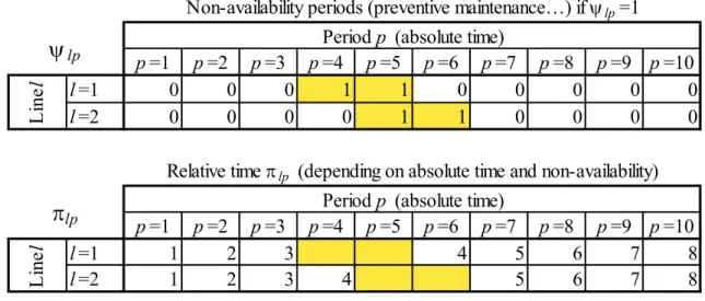
In MILP, time is defined with periods (e.g. hours) and not with dates. As non-availability periods are planned in the lines (mainly for preventive maintenance purposes…), the absolute period index p (p =1..P) must be replaced by a relative period index π which depends on the lp line. Boolean ψlp =1 if line l is not available during period p, and 0, if it is; then we can write
0 1 lp t p lp lpψ p t π = ψ
= = −
∑
= .The use of relative periods is mandatory in case of order due dates,taken into account in our models, and if there are time constraints on some inputs and/or some outputs. In the problem under study, work interrupted by maintenance can be resumed without changing total processing time.
Table 3 Example of definition of relative time
1 2 3 4 5 6 7 8 9
Orders to launch or fictitious order
orders in progress new orders to launch fictitious orders orders in progress or to launch
O' E EO′′ O E O′′′ E p =1 p =2 p =3 p =4 p =5 p =6 p =7 p =8 p =9 p =10 l =1 0 0 0 1 1 0 0 0 0 0 l =2 0 0 0 0 1 1 0 0 0 0 p =1 p =2 p =3 p =4 p =5 p =6 p =7 p =8 p =9 p =10 l =1 1 2 3 4 5 6 7 8 l =2 1 2 3 4 5 6 7 8
Relative time πlp (depending on absolute time and non-availability)
π
lp Period p (absolute time)Lin
e l
Non-availability periods (preventive maintenance…) if ψlp=1 Period p (absolute time)
Lin
e l
Decision variables
Two models are introduced. In both models, the orders inherit information from the references to produce. The table of notations, given in annex, makes explicit this mechanism. Boolean parameter βlj =1 if the output reference r required by order j (information given by
table Rj) can be produced by line l. Production rate ωlj of order j on line l copies that of
reference r on line l. Setup times λ involved by a change of output reference from one order lij to the following one on the same line; it copies that of the setup time involved by producing reference Rj after reference Ri on line l. The total production time θlij of order j following
order i on line l is the sum of the setup time λ and of the processing time lij φlj calculated as the quotient of the ordered quantity by the production rate of the reference r on line l. This preliminary transformation simplifies the two versions of our scheduling model.
In model 1, the binary decision variable x =lij 1 if order j (j ∈EO''') is processed on line l just
after order i (i ∈EO); in this formulation, time is indirectly addressed through precedence constraints in production (see relation (9)). The variable xlij exists only if β 1li= and βlj =1. Relation (1) defines the predicate H1 associated with the set of the decision variables xlij that
makes sense. This is very helpful when using Algebraic Modeling Languages (AML), like Xpress-IVE or GAMS.
O O''' 1
, , βli 1 βlj 1
l i j i∈ ∧ ∈E j E ∧ ≠ ∧i j = ∧ = ⇒H =True
(1) In model 2, the binary decision variable x =lijp 1 if order j (j ∈EO''') is processed on line l just after order i (i ∈EO), its last production period being p. Relation (2) defines the predicate H2
associated with the set of decision variables xlijp that makes sense. Note that this predicate includes the due date boundaries.
O O''' 2
, , , βli 1 βlj 1 Ilj πlp Slj
l i j p i j i≠ ∧ ∈ ∧ ∈E j E ∧ = ∧ = ∧ ≤ ≤ ⇒H =True (2)
In both models, the delivery dateyj is a decision variable corresponding to the last period of production of order j. In model 1, this variable is real; it is integer in model 2. The links between
j
y and xlij or xlijp are explained below.
Two other decision variables may be added in model 2. They reflect additional constraints and may be used in the optimization criterion. The first one is makespan Μ, defined as the latest delivery date among the scheduled orders (see relation 16). The second ones relates to consumption of a critical input, pulled by the schedule, and is the peak Π of its consumption (see relation 13).
Assignment constraints
A new or fictitious order j (j ∈EO''') is allocated to a single line ( 1..L)l = . An order in
progress at the beginning of the scheduling (j ∈EO') cannot be followed by more than one new
order and may be followed by no order if that line is not used in the schedule. This is enforced by relations (3) for model 1 and (4) for model 2.
1 1
O , l i, True lij 1 ; O', l i, True lij 1
j ′′′ = x i = x
∀ ∈E
∑
K = ∀ ∈E∑
K ≤(3)
2 2
O , l j p, , True lij lp 1 ; O', l j p, , True lij lp 1
i ′′′ = x π i = x π
∀ ∈E
∑
K = ∀ ∈E∑
K ≤(4)
Respect of delivery windows
The last period of production of order j is its delivery dateyj. This date is bounded by lower and upper dates (Llj and Ulj) that are defined with the relative calendar of line l. These constraints are enforced for the new orders ( )EO′′ in model 1 by relation (5) and, in model 2, by
relation (2) which restrains the scope of variable xlijp. Note that the delivery dates of the orders in progress are already known (∀ ∈j EO′,yj =Ljj =U )jj .
1 1
O , l i j, , TrueLlj lij j l i j, , TrueUlj lij
j ′′ = x y = x
∀ ∈E
∑
K ⋅ ≤ ≤∑
K ⋅(5)
A new order j produced on line l must have a predecessor i (in progress or new) produced on the same line. Relation (6) for model 1 and (7) for model 2 enforce order i to be produced on line l if x =lij 1(model 1) or
∑
pxlijπlp =1 (model 2).O O''' O'' βlj 1, k k j β 1lk lkj h h j β 1lh ljh j l ∈ ≠ ∧ = x ∈ ≠ ∧ = x ∀ ∈E ∧ ∀ =
∑
E =∑
E (6) O O'' βlj 1, k k j β 1lk p Llj lp Ulj lkj lp j l ∈ ≠ ∧ = ≤π ≤ x π ∀ ∈E ∧ ∀ =∑
E∑
= O''' β 1lh Llj lp Ulj ljh lp h∈ h j≠ ∧ = p ≤π ≤ x π∑
E∑
(7) Non-overlapping constraintsRelations (8) for model 1 and (9) for model 2 prevent order j from being produced as long as the production of order i is in progress, when both orders are produced on the same line. In these relations, the number P of periods plays the role of the “big M” constant.
1 1
O, O'' , j i l Trueθlij lij P (1 l True lij)
i j i j y y = x = x
∀ ∈E ∈E ≠ − ≥
∑
K ⋅ − ⋅ −∑
K(8)
2 2
O, O'' , j i l p, Trueθlij lij lp P (1 l p, True lij lp)
i j i j y y = x π = x π
∀ ∈E ∈E ≠ − ≥
∑
K ⋅ − ⋅ −∑
K(9)
Consideration of the upstream and downstream constraints (model 2)
Relations (10) to (16) are specific to model 2. Relation (10) links variables yj and xlijπlp in
2
O'', j l i p, , True lp lij lp
j y = π x π
∀ ∈E =
∑
K ⋅(10) Let’s take into account the incidence of the schedule on the consumption of an input regarded as critical (upstream consequences) and on the use of the inventories of the different produced qualities of fertilizers (downstream consequences).
Relation (11) defines total consumption Cp during period p of the input regarded as critical. It is a linear expression of the decision variables and uses the consumption rate qlj of order j
on line l (null if Ψ =lp 1). Cp is calculated as the sum of the consumption of orders in progress
(first part of the relation) and of new orders.
O ' , =0 π U , q lp lp j p l j l j lj p C ∈ = ∧Ψ ∧ ≤ ∀ =
∑
+ E O '' O , lj 1 lp=0 π Ulj jqlj , β 1li L π πj lt lp φlj lij lt l j∈ β = ∧Ψ ∧ ≤ ⋅ t p i≥ ∈ = ∧ ≠ ∧i j ≤ < + x π∑
E∑
E (11)Assuming that one knows the evolution Kp of the inventory of the input regarded as critical,
leaving aside the incidence of the schedule to find, relation (12) prevents from the risk of production stoppage due to input stockout. Note that the generalization of the model to consider all inputs is obvious but it increases the size of the problem needlessly in most cases.
1 K t p p p t C = = <
∑
(12)One can determine the maximum of peak Π of consumption of the input regarded as critical with relation (13) if the optimization criterion is that of relations 25 or 26
, p
p C
∀ ≤ Π (13)
Order j relates to quality output r (given by Rj) and several orders may relate to a single quality reference r. With production ratio plj on line l, total production Prp, during period p is
evolution Λrp of the inventory of reference r, leaving aside the incidence of the schedule to find, and the maximum level max
r
Λ that the inventory cannot exceed, relation (15) prevents a schedule to be unfeasible due to a saturation of the stock.
O ' O '' O , R = =0 U , 1 R = =0 U , 1 L , , p p j lp lp j lt lj j lp lj j li j lt lp lj rp l j l j r lj lj lij l j r t p i i j p r P x π π β π β π π ϕ ∈ = ∧ ∧Ψ ∧ ≤ ∈ = ∧ ∧Ψ ∧ ≤ ≥ ∈ = ∧ ≠ ∧ ≤ < + ∀ = + ⋅
∑
∑
∑
E E E (14) max , , t p rp rp r r p ≤ P ∀∑
+ Λ < Λ (15)The introduction of makespan Μ leads to its determination by relation (16)
2 C'', l i p, , True lijπlp j = p x ∀ ∈
∑
⋅ ≤ Μ K E (16) Optimization criteriaThe schedule cost is given by relation (17) for model 1 and (18) for model 2, where γ is lij the cost of producing order j on line l, after order i. These costs does not take into account expenses which must be supported whatever the decision taken; this point will be discussed under §III.3.
1
1 , ,
C =
∑
l i jK =Trueγlij⋅xlij (17)2
1 , , ,
C′ =
∑
l i j pK =Trueγaij⋅xlijπlt (18)Several schedules may have the same minimum value of C , because slacks can exist 1 between orders sequenced on the same line (in model 1, the decision variable yj being real, the number of equivalent schedules may be infinite). Among them, schedules with the earliest delivery dates are usually preferred, to keep the productive system busy in the short term. This is obtained by adding a penalty Κ (relation 19), weighted by the coefficient α, to C , which 1
gives criterion C (relation 21) to be used in model 1; in model 2, the penalty 2 Κ′(relation 20) is added to C′, to give criterion 1 C′ (relation 22). The value of α must be low enough not to 2 modify the values of order variables xlijor xlijπlt. The aim is to drive the choice of schedule
from the set of optimal schedules. The value of coefficient β j (0≤βj ≤1) aims to pull order j toward its earliest schedule when βj =1 and to push it toward its earliest schedule; if βj =0. The desired result is not achieved when conflicts occur between orders scheduled on the same line; in this case, one needs to work out the best schedule among the optimal ones.
1 1 C j ( j , Llj lij) C (1 j) ( , Ulj lij j) j∈ ′′β y l i =True x j∈ ′′ β l i =True x y Κ =
∑
⋅ −∑
⋅ +∑
− ⋅∑
⋅ − K K (19) 2 2 C j ( j , , , Llj lij lt) C (1 j) ( , , , Ulj lij lt j) j∈ ′′β y l i j p =True x π j∈ ′′ β l i j p =True x π y ′ Κ =∑
⋅ −∑
⋅ +∑
− ⋅∑
⋅ − K K (20) 2 1 C =C + ⋅Κα (21) 2 1 C′ =C′+ ⋅Κα ′ (22)Using model 2, one may prefer to minimize the consumption peak of the input regarded as critical, regardless of cost considerations. This leads to minimize relation 23 or 24.
Μ (23)
α ′
Μ + ⋅Κ (24)
One may also prefer to minimize the makespan, regardless of cost considerations, which leads to minimize relation 25 or 26
Π (25)
α ′
III.3 Numerical example
A small fictitious example is provided to illustrate both models.
Model 1
As in table 3, the scheduling problem deals with 2 lines (with the maintenance program of table 2) and 7 orders. These orders relate to 3 output references (Rj). Some of these references cannot be produced on all the lines. Tables 4 show for each order j and each line l, the upper and lower boundaries of the due dates (Llj and Ulj), the production rates plj of the order, the consumption rate ωlj of the critical input, the processing times φlj; setup time is assumed to
be 2 hours, whatever the sequence i→ j (i j≠ ) and whatever line l where j is produced. The cost function is γlij =10 φ 10 β β⋅ lj+ ⋅ ⋅li lj.
Tables 4: Scheduling problem data
Using criterion (21) with α =0.01 and βj = ∀1, j, we obtain the optimal solution, illustrated
by the Gantt in figure 1, where: x1,1,4 =x1,4,6 =x1,6,3 =x1,3,8=x2,2,5 = x2,5,7 =x2,7,9 =1 (the other decision variables being nil), C2 =574.32 and C 5741 = . Order 5 cannot start before period
11, which induces a “hole” in the Gantt. The calculus of the input consumption and the output productions are performed aside, as model 1 does not consider the upstream and downstream schedule impacts.
j =1 j =2 j =3 j =4 j =5 j =6 j =7 j =1 j =2 j =3 j =4 j =5 j =6 j =7 j =1 j =2 j =3 j =4 j =5 j =6 j =7
Line l= 1 5 0 12 8 0 6 9 Line l= 1 100 0 160 100 0 160 160 Line l= 1 50 0 64 50 0 64 64 Line l= 2 0 7 16 0 10 8 12 Line l= 2 0 80 120 0 80 120 120 Line l= 2 0 38 48 0 38 48 48 Rj (output) A B C A B C C φlj ωlj plj j =1 j =2 j =3 j =4 j =5 j =6 j =7 j =8 j =9 j =1 j =2 j =3 j =4 j =5 j =6 j =7 j =8 j =9 Line l= 1 7 0 10 15 0 20 30 1 0 Line l= 1 7 0 40 40 0 40 40 40 0 Line l= 2 0 9 10 0 20 20 30 0 1 Line l= 2 0 9 40 0 40 40 40 0 40 Llj Ulj 1 2 3 4 5 6 7 8 9 10 11 12 13 14 15 16 17 18 19 20 21 22 23 24 25 26 27 28 29 30 31 32 33 34 35 Line l=1 1 (A) 1 (A)
Figures 1: Optimal solution of model 1
Model 2
Using criterion (24) related to the consumption peak of the input regarded as critical, with
0.01
α = and βj = ∀1, j, we obtain the optimal solution, illustrated by the Gantt in figure 2, where x1,1,3,21=x1,3,6,27=x1,6,4,37=x1,4,8,38=x2,2,5,22=x2,5,7,39=x2,7,9,40=1 (the other decision variables being nil). We note a cost increase of 10 due to additional production launch versus the schedule yielded by model 1 and a consumption peak dropping to 240. Use of this criterion leads to an efficiency loss, (poor use of plant 2) and postpones by 5 hours the completion date for all the orders.
Figures 2: Optimal solution of model 2
III.2 Valuation System Used
Search for a solution to reduce operating cost of a production system is pointless if the savings theoretically afforded by the new solution do not show up in the corporate results. In
0 50 100 150 200 250 300 1 2 3 4 5 6 7 8 9 10 11 12 13 14 15 16 17 18 19 20 21 22 23 24 25 26 27 28 29 30 31 32 33 34 35 Period
Evolution of input consumption
0 20 40 60 80 100 120 Period
Evolution of production of outputs
Output A Output B Output C
1 2 3 4 5 6 7 8 9 10 11 12 13 14 15 16 17 18 19 20 21 22 23 24 25 26 27 28 29 30 31 32 33 34 35 36 37 38 39
I
II 2 (B) 2 (B) 5 (B) 7 ( C)
other words, an optimization model that matches reality adequately but relying on an irrelevant cost system is devoid of operational value.
The downside of using inadequate management accounting was pointed out at the end of the 1980’s and summarized by Johnson and Kaplan (1991), which led to the emergence of activity accounting (Activity Based Costing, ABC) popularized by many textbooks and in particular that of Kaplan & Cooper (1997). Rather than using standard costs, quotient of expenses by a produced quantity, this approach relies on the cost driver concept. Its use should be tailored to the context of transformation of a production system, since a number of expenses are not impacted by the decisions taken. It follows that one must develop an activity valuation model based on processes and stemming from the recommendations issue out of Supply Chain Costing (Seuring, 2002). Building a valorization system for operational management purposes in relation to hybrid production supply chains is a major issue (Degoun et al., 2015).
Fertilizer plant scheduling decisions are taken with reference to a temporal timeframe that is limited to four weeks. In this timeline, the number of lines open and the number of shifts operating them are known; the scheduling decisions are designed to use this production potential, without any impact whatsoever on these expenses as these must be considered to be fixed on this time horizon. Setup time corresponds to line cleaning time. Payroll cost does not feature since it is part of fixed expenses for the period; on the other hand, the cost of raw material wasted in the cleaning process and that of the cleaning products (mainly water) must be taken into account; the cost driver therefore clearly is the switch to a new reference for that line. Moreover, lines 07 and 107 have different performances levels. The difference of manufacturing rate for a fertilizer reference only impacts order delivery time and thus on the production means used. Between these types of lines, one observes slight differences on production BOM’s: to manufacture one tonne of a given fertilizer reference at workshop 07, versus workshop 107, one requires a little more raw materials (the difference can amount to up
to 0.5 %) and a little more power. Here the cost driver is clearly amount produced in a particular workshop. In principle, no other expense varies based on the selected scheduling solution.
The inclusion of these drivers in schedule choice, actually yields possible differences in actual expenditure.
DSS Description
The DSS prototype (Azzamouri et al., 2016) rests on a relational database comprising a number of structural data (production system description, routings, BOMs, costs) and data used to define a semi-structured problem: orders, preventive maintenance, forecasted trends − excluding impact of the schedule to be obtained − of raw material inventories used and of fertilizer reference inventories. An initial Java DSS interface module is used to update the database implemented under MySQL.
The next module of this interface is used to define the semi-structured problem to be dealt with (component 1 of SAD), serving to perform an initial feasibility check, and then to define a structured problem to be solved with model 1 (the possible use of model 2 is not useful due to large calculation time) and to generate a data file to be used to create a problem instance of the generic problem defined under Xpress-IVE, before launching the problem resolution (component 2 of DSS). A third module uses the results of the optimization to assess feasibility in relation to impact upstream and downstream of SC (component 3 of DSS). If the solution is deemed not feasible, this leads to revising the issue to be optimized (component 4 of DSS). The retroaction of analysis of a solution that was found with model 1 (component 4 of SAD) on the reformulation of a semi-structured issue (component 1 of SAD) mainly concerns the definition of the date windows for completion of production of orders and on the weighting coefficients leading orders to be scheduled preferably either soonest or latest. It also may lead to a break up of orders in order to meet a delivery date where it appears that the production
potential is under-utilized or to adjust the preventive maintenance schedule. The following figure summarizes DSS operation.
OCP’s CL comprises a number of parallel axes. Two of them, the Northern axis (Jorf) and the central axis possess a fertilizer production plant. The proposed approach can easily be tailored to enable global, therefore more efficient, management of fertilizer production in these plants.
Conclusion
A prototype of Decision Support System is about to be experimented with some actual problems, which is a mandatory step before its implementation in the fields. Two
complementary extensions are studied: the first one aims to merge the scheduling of two distant fertilizer plants to improve their capacity use (see above); the second aims to lengthen the schedule horizon to be able to include possible orders and help the sales department negotiate the best compromise between price and delivery time.
References
VI.1 References used in table 1
1. Adamopoulos, G., Pappis, C. 1998. “Scheduling under a common due-date on parallel unrelated machines”. European Journal of Operational Research 105, 494–501. 2. Anghinolfi, D., Paolucci, M. 2007. “Parallel machine total tardiness scheduling with a
new hybrid metaheuristic approach”. Computers and Operations Research 34, 3471– 3490.
3. Behnamian, J., Zandieh, M., Ghomi, S.M.T.F. 2010. “Due window scheduling with sequence-dependent setup on parallel machines using three hybrid metaheuristic algorithms”. International Journal of Advanced Manufacturing Technology 44, 795– 808.
4. Bin, F., Yumei, H., Hairong, Z. 2011. “Approximation schemes for parallel machine scheduling with availability constraints. Discrete Applied Mathematics” 159, 1555– 1565.
5. Cao, D., Chen, M., Wan, G. 2005. “Parallel machine selection and job scheduling to minimize machine cost and job tardiness”. Computers & Operations Research 32, 1995–2012.
6. Chen, J.-F. 2005. “Unrelated parallel machine scheduling with secondary resource constraints”. International Journal of Advanced Manufacturing Technology 26, 285– 292.
7. Chen, J.-F., Wu, T.-H. 2006. “Total tardiness minimization on unrelated parallel machine scheduling with auxiliary equipment constraints”. Omega 34, 81–89.
8. De Paula, M.R., Mateus, G.R., Ravetti, M.G. 2010. “A non-delayed relax-and-cut algorithm for scheduling problems with parallel machines, due dates and sequence-dependent setup times”. Computers and Operations Research 37, 938–949.
9. Dong-Won, K., Kyong-Hee, K., Wooseung, J., Chen, F. 2002. “Unrelated parallel machine scheduling with setup times using simulated annealing”. Robotics and
Computer-Integrated Manufacturing 18, 223–231.
10. Fang, K.-T., Lin, B.M.T. 2013. “Parallel-machine scheduling to minimize tardiness penalty and power cost”. Computers & Industrial Engineering 64, 224–234.
11. Gabrel, V. 1995. “Scheduling jobs within time windows on identical parallel machines: New model and algorithms”. European Journal of Operational Research 83, 320–329. 12. Gacias, B., Artigues, C., Lopez, P. 2010, “Parallel machine scheduling with precedence
13. Guinet, A. 1993. “Scheduling sequence-dependent jobs on identical parallel machines to minimize completion time criteria”. International Journal of Production Research 31, 1579–1594.
14. Hashemian, N., Diallo, C., Vizvári, B. 2014. “Makespan minimization for parallel machines scheduling with multiple availability constraints”. Annals of Operations
Research 213, 173–186.
15. Hidri, L., Gharbi, A., Haouari, M. 2008. “Energetic reasoning revisited: application to parallel machine scheduling”. Journal of Scheduling 11, 239–252.
16. Jeng-Fung Chen. 2010. “Scheduling on unrelated parallel machines with sequence- and machine-dependent setup times and due-date constraints”. International Journal of
Advanced Manufacturing Technology 44, 1204–1212.
17. Kim, D.-W., Na, D.-G., Frank Chen, F. 2003. “Unrelated parallel machine scheduling with setup times and a total weighted tardiness objective”. Robotics and
Computer-Integrated Manufacturing, 12th International Conference on Flexible Automation and
Intelligent Manufacturing 19, 173–181.
18. Lee, C.-Y. 1991. “Parallel machines scheduling with non-simultaneous machine available time”. Discrete Applied Mathematics 30, 53–61.
19. Lee, H.-T., Yang, D.-L., Yang, S.-J. 2013. “Multi-machine scheduling with deterioration effects and maintenance activities for minimizing the total earliness and tardiness costs”. International Journal of Advanced Manufacturing Technology 66, 547–554.
20. Lee, J.-H., Yu, J.-M., Lee, D.-H. 2013. “A tabu search algorithm for unrelated parallel machine scheduling with sequence- and machine-dependent setups: minimizing total tardiness”. International Journal of Advanced Manufacturing Technology 69, 2081– 2089.
21. Liao, C..-J., Chen, C.-M., Lin, C.-H. 2007. “Minimizing Makespan for Two Parallel Machines with Job Limit on Each Availability Interval”. The Journal of the Operational
Research Society 58, 938–947.
22. Liao, C.-J., Shyur, D.-L., Lin, C.-H. 2005. “Makespan minimization for two parallel machines with an availability constraint”. European Journal of Operational Research, Decision Support Systems in the Internet Age 160, 445–456.
23. Lin, S.-W., Lu, C.-C., Ying, K.-C. 2011. “Minimization of total tardiness on unrelated parallel machines with sequence- and machine-dependent setup times under due date constraints”. International Journal of Advanced Manufacturing Technology 53, 353– 361.
24. Lin, S.-W., Ying, K.-C. 2014. “ABC-based manufacturing scheduling for unrelated parallel machines with machine-dependent and job sequence-dependent setup times”.
Computers & Operations Research 51, 172–181.
25. Ma, Y., Chu, C., Zuo, C. 2010. “A survey of scheduling with deterministic machine availability constraints”. Computers & Industrial Engineering 58, 199–211.
26. Moon, J.-Y., Shin, K., Park, J. 2013. “Optimization of production scheduling with time-dependent and machine-time-dependent electricity cost for industrial energy efficiency”.
27. Nait Tahar, D., Yalaoui, F., Chu, C., Amodeo, L. 2006. “A linear programming approach for identical parallel machine scheduling with job splitting and sequence-dependent setup times”. International Journal of Production Economics, Control and Management of Productive Systems Control and Management of Productive Systems 99, 63–73.
28. Obeid, A., Dauze`re-Pe´re`s, S., Yugma, C. 2014. “Scheduling job families on non-identical parallel machines with time constraints”. Annals of Operations Research 213, 221–234.
29. Pereira Lopes, M.J., de Carvalho, J.M.V. 2007. “Discrete Optimization: A branch-and-price algorithm for scheduling parallel machines with sequence dependent setup times”.
European Journal of Operational Research 176, 1508–1527.
30. Rocha, P.L., Ravetti, M.G., Mateus, G.R., Pardalos, P.M. 2008. “Exact algorithms for a scheduling problem with unrelated parallel machines and sequence and machine-dependent setup times”. Computers and Operations Research 35, 1250–1264.
31. Rodrigues, R. de F., Dourado, M.C., Szwarcfiter, J.L. 2014. “Scheduling problem with multi-purpose parallel machines”. Discrete Applied Mathematics, Combinatorial
Optimization 164, Part 1, 313–319.
32. Schutten, J., Leussink, R. 1996. “Parallel machine scheduling with release dates, due dates and family setup times”, International Journal of Production Economics. 46, 119–125.
33. Suk, J., Kyung, K. 2008: “Parallel machine scheduling with earliness-tardiness penalties and space limits”. International Journal of Advanced Manufacturing
Technology 37, 793–802.
34. Vallada, E., Ruiz, R. 2011. “A genetic algorithm for the unrelated parallel machine scheduling problem with sequence dependent setup times”. European Journal of
Operational Research 211, 612–622.
35. Van Hop, N., Nagarur, N.N. 2004. “The scheduling problem of PCBs for multiple non-identical parallel machines”. European Journal of Operational Research 158, 577–594. 36. Weng, M.X., Lu, J., Ren, H. 2001. “Unrelated parallel machine scheduling with setup consideration and a total weighted completion time objective”. International Journal of Production Economics 70, 215–226 (2001)
37. Xi, Y., Jang, J. 2012. “Review: Scheduling jobs on identical parallel machines with unequal future ready time and sequence dependent setup: An experimental study”.
International Journal of Production Economics 137, 1–10.
38. Young Hoon Lee, Pinedo, M. 1997. “Scheduling jobs on parallel machines with sequence-dependent setup times”. European Journal of Operational Research 100, 464–474.
39. Zhao, C., Ji, M., Tang, H. 2011. “Parallel-machine scheduling with an availability constraint”. Computers & Industrial Engineering 61, 778–781.
40. Zhu, Z., Heady, R.B. 2000, “Minimizing the sum of earliness/tardiness in multi-machine scheduling: a mixed integer programming approach”. Computers & Industrial
Engineering 38, 297–305.
41. Giard V., Azzamouri A., Essaadi I. 2015, “Définition d’un SIAD d’ordonnancement sur processeurs parallèles hétérogènes, avec prise en compte de fenêtre de fin de
production, de plages d’indisponibilités des processeurs et de temps de lancement
dépendant du processeur et de la sequence”. Cahier du LAMSADE 369
(http://www.lamsade.dauphine.fr/sites/default/IMG/pdf/cahier_369.pdf)
VI.2 Other references
Azzamouri, A., Essaadi, I., Fénies, P., Fontane, F., Giard, V. 2016. “Définition d’un Système d’Aide à la Décision d’ordonnancement des commandes sur les lignes de l’atelier d’engrais”, RIRL 2016 . (Rencontres Internationales de la recherche en logistique).
Eom, S., Kim, E. 2006. “A Survey of Decision Support System Applications (1995–2001)”.
Journal of the Operational Research Society 57 (11), 1264-1278.
Bhargava, H.K, Power, D.J, Sun, D. (2007). “Progress in Web-based decision support technologies”, Decision Support Systems. 43 (4), 1083-1095.
Degoun M., Fenies P., Giard V., Retmi K., Saadi J., (2015). “Évaluation de la performance économique d’une chaîne logistique hybride”, Congrès de Génie Industriel (CIGI), Montréal, Octobre 2015.
Giard, V., Azzamouri, A., Essadi, I. (2016). “A DSS approach for heterogeneous parallel machines scheduling with due windows, processor-&-sequence-dependent setup and availability constraints”, Information System, Logistics and Supply (ILS 2016).
Johnson H. T., Kaplan, R. S. (1991). Relevance Lost: The Rise and Fall of Management
Accounting, Harvard Business Press.
Kaplan, R. S., Cooper, R. (1997). Cost & Effect: Using Integrated Cost Systems to Drive
Profitability and Performance, Harvard Business School Press
Keen, P., Scott Morton, M. (1978). Decision Support Systems: An Organizational Perspective, Addison-Wesley Publishing, Reading, MA.
Gorry, G.A., Scott Morton, M.S. (1971). A framework for management, information systems,
Sloan Management Review 13 (1).
Power, D.J., Sharda, R. (2007). “Model-Driven Decision Support Systems: Concepts and Research Directions.” Decision Support Systems 43 (3), 1044–1061.
Seuring, S. (2002) Supply Chain Costing- A conceptual framework, in Cost Management in
Supply Chains, Seuring S. et Goldbach M. editors, Springer, p.15–30.
Shim, J.P., Warkentin, M., Courtney, J.F., Power, D.J., Sharda, R., Carlsson, C. 2002. Past, Present, and Future of Decision Support Technology. Decision Support Systems 33, 111– 126.
Table of notations
In this table, we present primary information of orders, BOM and routing used to calculate the model parameters (they are not used in the model). The retained time bucket is one hour in the table (in accordance with the data of the actual problem) but this unit can easily be changed.
o
i, j
Subscript of an order (o =1..O)
Set EO defined for o =1..L; set EO' defined for o = +L 1..O; set EO′′
defined for o =O+1..O+L; set EO′′′defined for o =L+1..O+L
Subscript of a scheduled order on a given line, order i being directly followed by order j
l Subscript of a parallel line ( 1..L)l =
p Subscript of absolute period (p =1..P)
lp
π Subscript of relative period for line l corresponding to the absolute period
p; it takes into account the periods during which line l is not available
(preventive maintenance…) 0 1 lp t p lp lpψ p t π = ψ = = −
∑
=r Subscript of an output reference
r is used in the creation of the problem data but not in the model
TECHNICAL PARAMETERS
lp
ψ Binary parameter = 1 if line l is unavailable during period p
Rj Reference to produce for order j
is used in the creation of the problem data but not by the model β′ lr Binary parameter = 1 if the output reference r required by order j can be
produced by line l
is used in the creation of the problem data but not by the model
βlj Binary parameter = 1 if the order j can be produced by line l (βlj =β )l′Rj
ωlr′ Production rate of output r on line l (in tonnes/hour)
is used in the creation of the problem data but not by the model
ωlj Production rate of order j on line l (ωlj =ωl′Rj)
is used in the creation of the problem data but not by the model
Qj Quantity to produce for order j
Qj is used in the creation of the problem data but not by the model
φlj Processing time of order j on line l (φlj = Q / ω )j lj , excluding setup time
Rj
βlr′
ωlr′
Expressed in hours (with the definition of the production rate)
1 2 lr r
λ′ Setup time for producing the reference r after the reference 2 r on line l 1
1 2 lr r
λ′ is used in the creation of the problem data but not by the model
lij
λ Setup time for producing the reference j after the reference i on line l
R Ri j
lij l
λ =λ′ is used in the creation of the problem data but not by the model
θlij Total processing time of order j produced on line l after order j, including setup time
θlij =φlj+λlij
Llj Lower boundary of the last period of production for order j ( )yj ; it uses the
relative period index of line l where this order is produced
Ulj Upper boundary of the last period of production of order j ( )yj ; it uses the
relative period index of line l where this order is produced
rp
Λ Evolution of the inventory of output r, leaving aside the incidence of the schedule to find
Used only in model 2 max
r
Λ Maximum level that the inventory of output r cannot exceed
Used only in model 2
Kp Evolution of the inventory of the input regarded as critical, leaving aside the incidence of the schedule to be found
Used only in model 2 COSTS
1 2 lr r ′
Λ Setup cost induced by the production of the reference r after the 2
reference r on line l 2
1 2 lr r ′
Λ is used in the creation of the problem data but not by the model
lij
Λ Setup cost induced by the production of order j after order i on line l
R Ri j
lij l′
Λ = Λ is used in the creation of the problem data but not by the model
lr
Γ Direct variable cost induced by the production of one hour of reference r on
line l
lr
γlij Production cost of Qj in line l γlij = Γ ⋅lRj φlj+ Λlij
α Low coefficient applied to the penalty cost added to the objective function
1
C to drive the choice of the schedule among the set of optimal schedules, in case of slack in production schedule
j
β Coefficient used to drag the schedule of order j towards its earliest value or its latest possible value in case of slack;0≤βj ≤1
DECISION VARIABLES
lij
x Binary decision variable = 1 if order j (j ∈EO''') is processed on line l just after order i (i ∈EO)
Used only in model 1
lijp
x Binary decision variable = 1 if order j (j ∈EO''') is processed on line l just after order i (i ∈EO)
Used only in model 2
j
y Date of the end of production of order j; it uses the relative period index π lp of line l where this order is produced
j
y is a real variable in model 1 and integer variable in model 2
Μ Makespan (Μ =Max y( ))j
Used only in model 2
Κ Maximum consumption of the input regarded as critical involved by the
schedule solution