HAL Id: pastel-00003506
https://pastel.archives-ouvertes.fr/pastel-00003506
Submitted on 27 Jul 2010
HAL is a multi-disciplinary open access
archive for the deposit and dissemination of sci-entific research documents, whether they are pub-lished or not. The documents may come from teaching and research institutions in France or abroad, or from public or private research centers.
L’archive ouverte pluridisciplinaire HAL, est destinée au dépôt et à la diffusion de documents scientifiques de niveau recherche, publiés ou non, émanant des établissements d’enseignement et de recherche français ou étrangers, des laboratoires publics ou privés.
Pointer Analysis and Separation Logic.
Elodie-Jane Sims
To cite this version:
Elodie-Jane Sims. Pointer Analysis and Separation Logic.. Computer Science [cs]. Ecole Polytech-nique X, 2007. English. �pastel-00003506�
TH`
ESE
pr´esent´ee `a
l’´
ECOLE POLYTECHNIQUE
pour l’obtention du titre de
DOCTEUR DE L’´
ECOLE POLYTECHNIQUE
EN INFORMATIQUE
´
Elodie-Jane Sims
1er d´ecembre 2007
Analyses de Pointeurs et Logique de
S´
eparation
Pointer Analysis and Separation Logic
Pr´esident: Reinhard Wilhelm
Professeur, Universit¨at des Saarlandes, Saarbr¨ucken, Allemagne
Rapporteurs: Hongseok Yang
Queen Mary, University of London, London, Royaume Uni
Reinhard Wilhelm
Professeur, Universit¨at des Saarlandes, Saarbr¨ucken, Allemagne
Examinateurs: Roberto Giacobazzi
Professeur, Universita’ degli Studi di Verona, Italie
David Schmidt
Professeur, Kansas State University, Manhattan Kansas, USA
Directrice de th`ese: Radhia Cousot
Th`ese en co-tutelle ´Ecole Polytechnique (France) et Kansas State University (USA) sous la direction de Radhia Cousot, CNRS/ ´Ecole normale sup´erieure (France) et David Schmidt, Kansas State University (USA).
´
Ecole Polytechnique (France) and Kansas State University (USA) co-directed Ph.D de-gree under the direction of Radhia Cousot, CNRS/ ´Ecole normale sup´erieure (France) and David Schmidt, Kansas State University (USA).
Copyright
´
Elodie-Jane Sims
2007
R´
esum´
e
Le cadre de cette th`ese est l’analyse statique modulaire par interpr´etation abstraite de logiciels en vue de leur v´erification automatique. Nous nous int´eressons en particulier aux programmes comportant des objets allou´es dynamiquement sur un tas et rep´er´es par des pointeurs. Le but final ´etant de trouver des erreurs dans un programme (probl`emes de d´er´ef´erencements et d’alias) ou de prouver qu’un programme est correct (relativement `a ces probl`emes) de fa¸con automatique.
Isthiaq, Pym, O’Hearn et Reynolds ont d´evelopp´e r´ecemment des logiques de fragmen-tation (separation logics) qui sont des logiques de Hoare avec un langage d’assertions/de pr´edicats permettant de d´emontrer qu’un programme manipulant des pointeurs sur un tas est correct. La s´emantique des triplets de la logique ({P }C{P′}) est d´efinie par des trans-formateurs de pr´edicats de style plus faible pr´e-condition.
Nous avons exprim´e et prouv´e la correction de ces plus faibles pr´e-conditions (wlp) et plus fortes post-conditions (sp), en particulier dans le cas de la commande while. L’avantage par rapport `a ce qui est fait dans la communaut´e est que les wlp et sp sont d´efinis pour toute formule alors que certaines des r`egles existantes avaient des restrictions syntaxiques.
Nous avons rajout´e des points fixes `a la logique ainsi qu’une substitution retard´ee per-mettant d’exprimer des formules r´ecursives. Nous avons exprim´e les wlp et sp dans cette logique avec points fixes et prouv´e leur correction. La substitution retard´ee a une utilit´e directe pour l’expression de formules r´ecursives. Par exemple, nclist(x) = µXv. (x = nil) ∨ ∃x1, x2.(isval(x1) ∧ (x 7→ x1, x2 ∗ Xv[x2/x])) d´ecrit l’ensemble des m´emoires o`u x pointe vers une liste d’entiers.
Le but ensuite ´etait d’utiliser cette logique de fragmentation avec points fixes comme langage d’interface pour des analyses de pointeurs. Il s’agit de formuler une traduction
des domaines de ces analyses en formules de la logique (et inversement) et d’en prouver la correction. On peut ´egalement parfois utiliser ces traductions pour prouver la correction de ces analyses.
Nous avions d´ej`a illustr´e cette approche pour une analyse tr`es simple de partitionnement des pointeurs. Nous avons traduit les formules de la logique dans un nouveau langage abstrait permettant de d´ecrire le type des valeurs associ´ees aux variables dans la m´emoire (nil, entier, bool, pointeur vers une paire de tel type, etc.) ainsi que les relations d’aliasing et non-aliasing entre variables et entre points de la m´emoire. Le principal apport est la d´efinition de ce langage et de sa sa s´emantique dans le domaine concret qui est celui utilis´e pour la s´emantique des formules. En particulier, les variables auxiliaires dont la s´emantique est habituellement une question d’impl´ementation font ici explicitement part du langage et de sa s´emantique. Ce langage est un produit cartesien de plusieurs sous domaines et peut ˆetre param´etr´e par les domaines num´eriques existants. Nous avons cr´e´e un sous-domaine qui est un tableau permettant de compenser le manque de pr´ecision dˆu `a l’utilisation de graphes d’ensembles au lieu d’ensembles de graphes. Nous avons exprim´e et prouv´e les traductions des formules dans ce langage abstrait.
Abstract
We are interested in modular static analysis to analyse softwares automatically. We focus on programs with data structures, and in particular, programs with pointers. The final goal is to find errors in a program (problems of dereferencing, aliasing, etc) or to prove that a program is correct (regarding those problems) in an automatic way.
Isthiaq, Pym, O’Hearn and Reynolds have recently developed separation logics, which are Hoare logics with assertions and predicates language that allow to prove the correctness of programs that manipulate pointers. The semantics of the logic’s triples ({P }C{P′}) is defined by predicate transformers in the style of weakest preconditions.
We expressed and proved the correctness of those weakest preconditions (wlp) and strongest postconditions (sp), in particular in the case of while-loops. The advance from the existing work is that wlp and sp are defined for any formula, while previously existing rules had syntactic restrictions.
We added fixpoints to the logic as well as a postponed substitution which then allow to express recursive formulae. We expressed wlp and sp in the extended logic and proved their correctness. The postponed substitution is directly useful to express recursive formulae. For example, nclist(x) = µXv. (x = nil) ∨ ∃x1, x2.(isval(x1) ∧ (x 7→ x1, x2 ∗ Xv[x2/x])) describes the set of memory where x points to a list of integers.
Next, the goal was to use separation logic with fixpoints as an interface language for pointer analysis. That is, translating the domains of those analyses into formulae of the logic (and conversely) and to prove their correctness. One might also use the translations to prove the correctness of the pointer analysis itself.
We illustrate this approach with a simple pointers-partitioning analysis. We translate the logic formulae into an abstract language we designed which allows us to describe the
type of values registered in the memory (nil, integer, booleans, pointers to pairs of some types, etc.) as well as the aliasing and non-aliasing relations between variables and loca-tions in the memory. The main contribution is the definition of the abstract language and its semantics in a concrete domain which is the same as the one for the semantics of for-mulae. In particular, the semantics of the auxiliary variables, which is usually a question of implementation, is explicit in our language and its semantics. The abstract language is a partially reduced product of several subdomains and can be parametrised with existing numerical domains. We created a subdomain which is a tabular data structure to cope with the imprecision from not having sets of graphs. We expressed and proved the translations of formulae into this abstract language.
Contents
Table of Contents i List of Figures v Acknowledgements vi 1 Introduction 1 1.1 Motivations . . . 11.2 Introduction to separation logic . . . 5
1.3 History of the project and contributions . . . 11
1.4 Structure of the manuscript . . . 18
2 Separation logic with fixpoints 19 2.1 Commands and basic domains . . . 19
2.1.1 Command syntax . . . 19 2.1.2 Semantic domains . . . 20 2.1.3 Small-step semantics . . . 21 2.2 BIµν . . . . 22 2.2.1 Syntax of formulae . . . 22 2.2.2 Semantics of formulae . . . 23 2.2.3 Interpretation of Triples . . . 25
2.2.4 Fixpoints and postponed substitution . . . 26
2.3 Backward analysis . . . 33
2.4 Forward analysis . . . 34
2.5 Variations of BIµν . . . . 37
2.6 Appendix . . . 41
2.6.1 Definitions . . . 41
2.6.2 Stack Extension Theorem . . . 44
2.6.3 Variable Renaming Theorem for BIµν . . . . 48
2.6.4 Unfolding theorems . . . 55
2.6.5 Substitution theorems for BIµν . . . . 55
2.6.6 Substitution theorems for BIµν general . . . . 60
2.6.7 µ and ν coincide . . . 64
2.6.8 Simplifications on [ / ] . . . 65
2.6.9 sp’s proofs . . . 68
2.6.10 wlp’s proofs . . . 74
2.6.12 Simplification theorems . . . 82
3 An abstract language for separation logic 84 3.1 Introduction . . . 84
3.2 Examples: Introduction to the language, translations of formulae . . . 86
3.2.1 Full example: tree . . . 91
3.3 Definition of the language, AR . . . 92
3.4 Semantics of the language . . . 96
3.5 Operations on the language . . . 99
3.5.1 Extension . . . 100 3.5.2 Union . . . 103 3.5.3 Merging nodes . . . 107 3.5.4 Stabilization . . . 111 3.5.5 ast . . . 114 3.5.6 Intersection . . . 122 3.6 Translation of formulae . . . 127
3.6.1 Properties of the translation . . . 127
3.6.2 Translation of ∧ . . . 130 3.6.3 Translation of ∨ . . . 131 3.6.4 Translation of ∃ . . . 131 3.6.5 Translation of E1 = E2 . . . 132 3.6.6 Translation of x 7→ E1, E2 . . . 132 3.6.7 Translation of µ and ν . . . 133 3.7 Conclusion . . . 134 3.8 Appendix . . . 135 3.8.1 Replace . . . 135
3.8.2 Cheap extension proofs . . . 135
3.8.3 Extension proofs . . . 145
3.8.4 Union proofs . . . 155
3.8.5 Merging proofs . . . 158
3.8.6 Functions on CLeq proofs . . . 168
3.8.7 Widening proofs . . . 169
3.8.8 Basic ast proofs . . . 171
3.8.9 Extra ast proofs . . . 179
3.8.10 Basic equal proofs . . . 181
3.8.11 Reach functions proofs . . . 185
3.8.12 Class proofs . . . 188
3.8.13 Exists proofs . . . 192
4 Implementation 195
4.1 Introduction . . . 195
4.2 Software architecture . . . 196
4.2.1 Reading from files . . . 196
4.2.2 Computing informations . . . 197
4.2.3 Building executables . . . 198
4.3 Syntaxes of inputs and data structures . . . 198
4.3.1 Program syntax . . . 199
4.3.2 Formula syntax . . . 201
4.3.3 Abstract data syntax . . . 203
4.4 The translation of formula into elements of the domain: sl2ar.ml . . . 210
4.5 Analysis . . . 214
5 Comparison with other works 216 5.1 Smallfoot . . . 216
5.1.1 Smallfoot: Modular Automatic Assertion Checking with Separation Logic (FMCO’05) . . . 216
5.1.2 A local shape analysis based on separation logic (TACAS’06) . . . 219
5.1.3 Shape analysis for composite data structures (CAV’07) . . . 222
5.1.4 Footprint Analysis: A Shape Analysis that Discovers Preconditions (SAS’07) . . . 225
5.1.5 Conclusions about smallfoot/space invader . . . 228
5.2 TVLA . . . 228
5.3 others . . . 235
5.4 Conclusion . . . 235
5.4.1 Modularity . . . 236
5.4.2 Expressibility of heap logic . . . 236
5.4.3 Folding/unfolding . . . 237
5.4.4 Theorem provers . . . 238
5.4.5 Auxiliary variables . . . 238
5.4.6 Analysis versus verification . . . 238
5.4.7 What is distinctive about our system . . . 239
6 Conclusion 241
Bibliography 246
Appendix 246
A Junk: ast algorithm 247
B Intersection 254
List of Figures
1.1 Examples of separation formulae and memory satisfying them . . . 10
1.2 Example of separation logic formulae which caracterize a piece of code insert-ing a cell in a linked list, on the right is a graphical view of memory satifyinsert-ing the formulae . . . 12
1.3 Local reasoning: exemple of Fig. 1.2 for an extended heap . . . 13
2.1 Operational small-step semantics of the commands . . . 21
2.2 Semantics of BIµν . . . . 24
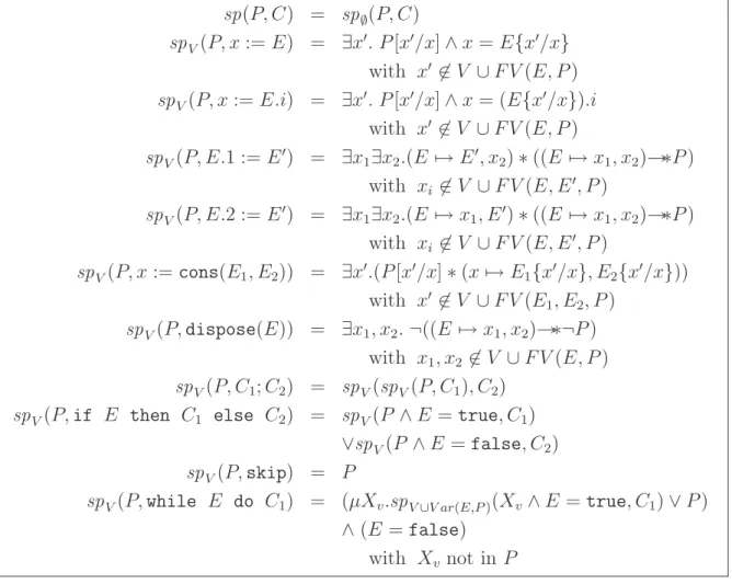
2.3 Weakest liberal preconditions . . . 35
2.4 Strongest postconditions . . . 38
3.1 Introduction examples . . . 86
3.2 Introduction examples . . . 87
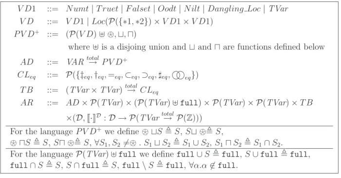
3.3 Syntax of the language . . . 93
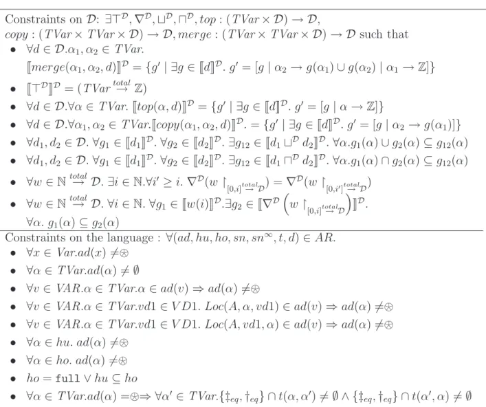
3.4 Constraints on the language . . . 94
4.1 Reading a program in a file . . . 197
4.2 Reading a formula in a file . . . 197
4.3 Computing pre- and post-conditions, computing the abstraction . . . 197
4.4 The executables produces by the analyses . . . 200
4.5 The result domain structure . . . 207
5.1 Table from the article . . . 220
5.2 Return of example for SAS’07 . . . 227
5.3 TVLA’s core predicates . . . 229
5.4 some TVLA’s instrumentation predicates . . . 230
5.5 TVLA’s formula syntax . . . 230
5.6 TVLA’s formula semantics . . . 231
5.7 TVLA’s list-reversal program . . . 232
5.8 TVLA’s list-reversal result of analysis . . . 233
5.9 TVLA’s example . . . 234
Acknowledgments
I would like to warmly thank all those I will not mention here and were there during this heavy period as a PhD student and in particular all those who went all the way up hill in the maze to attend my defense !
I am very proud that Reinhard Wilhelm and Hongseok Yang accepted to be my reviewers and grateful for the work they have done. I have been impressed by the interest and kindness they shown and the quality of their remarks. I would like to thank Roberto Giacobazzi for accepting to be a member of my jury, it was an honor.
The most important person involved in a PhD, after the student is its adviser. I was glad to be granted of two advisers, Radhia Cousot and David Schmidt. They both were very helpful, and supporting, in their own domains of action. I obviously wouldn’t have started this thesis without them, but I also wouldn’t have finished it ! My biggest thanks go for them.
I naturally come to thank Patrick Cousot after them, he is the one who introduced me to them both, and to my area of work. He also was a great scientific help and trigger during my DEA’s internship and at the very beginning of my thesis.
I was surprised to get so many and great gifts after my defense, but the best one was three big brothers: Charles Hymans, Georg Jung and Francesco Logozzo. I haven’t been as supportive to the youngest as I received, but I was very happy to be with Guillaume Capron and Pietro Ferrara. I believe co-PhDs remain co-PhDs after their defenses !
I was so lucky to have great colleagues and would like to thank: Anindya Banerjee, Julien Bertrane, Bruno Blanchet, Simon Bliudze, Gilles Dowek, J´erˆome Feret, Bertrand Jeannet, Gurvan Le Guernic, Mathieu Martel, Isabella Mastroeni, Laurent Mauborgne, Antoine Min´e, Alexander Serebrenik, Axel Simon, Allen Stoughton, Xavier Rival, Robby and Sarah Zennou.
I would like to thank Kansas State University and in particular CIS department, for their kindness when I was there and all the administrative organisation.
I am sincerely glad my family is there for me, in particular my american family who is so supportive from far away. Je tiens `a remercier mon grand-p`ere Andr´e Pichard qui fut mon mod`ele. Sans ma formidable grand-m`ere Jeanne Pichard, j’aurais fini cette th`ese transform´ee en pizza ! Je remercie ma grand-tante Paulette Cˆome pour son ´ecoute et ses encouragements. Je remercie ma m`ere Anne-Lise Pichard pour le soutien qu’elle a su m’apporter. Je tiens `a remercier mon affreuse frangine, Anne-Orlis Pigneur (et son mari Thomas), pour mon adorable ni`ece Mathilde, bon je plaisante, je la remercie aussi pour bien bien d’autres choses.
Last but not least. Je tiens `a remercier mes amis, mon plus important soutien, tout par-ticuli`erement ma meilleure amie Marion Martin dont le t´el´ephone a support´e mes lamentations journali`eres ! Je ne peux remercier ici que ceux qui m’ont promis des repr´esailles en cas d’oubli ;-) : No´emie Atlan, T´erence Bayen, Anne-Marie Bleau, Denis Conduch´e, Florian Douetteau, Cl´ementine Doumenc, Alain Frisch, C´eline Georgin, Jean-Marc L´eoni, Melanie Pfeiffer, Benoˆıt Piedallu, An-drea Platz, H´elo¨ıse Viard et Alexandra Vidalenc. I omit now unforgettable thanks.
Chapter 1
Introduction
1.1
Motivations
Programs (also called software) are used in many places in our environment and a big part of the effort of programing is used for the so called debugging part (finding errors). One massively used technique for debugging is testing (trying to run the program in various situations). Through testing, one can test only some values, thus testing never insures the program has no error. You can not try all integers before answering that the program works for all integers; you can not run the program forever before answering the program will run without error forever. When programs are used in critical situations (for example, in spaceships, public transportations, power plants, banking), it is then very important to insure their safety, and it is even sometimes mandatory by laws. Formal methods try to address the problem by providing mathematically sound techniques that guarantee a full coverage of all program behaviours.
We are interested in doing static analysis. This consists of proving a program’s correct-ness or other properties on the program without running the program. Running a program uses a domain called the operational domain (like values assigned to variables, having mem-ory locations, ...) and applies changes to elements of the domain following the instructions given by the program. Static analysis uses a domain which abstracts (“represents”) the op-erational domain and applies changes to elements on this abstracting domain. The changes
in the abstracting domain are related to the changes the program would operate on the operational domain so that at the end, knowing the changes in the abstracting domain gives us informations about how the program behaves on the operational domain.
Abstract interpretation1–3provides a framework which first helps proving that some
prop-erties on the abstracting domain (there called the abstract domain) implies some propprop-erties on the operational domain; secondly, it helps designing abstracting domains.
Here, we give an example for non computer scientists. Imagine a program that tries to compute an integer (a number). The program gives an error if it attempts to do a division by 0 since the result would be infinity, which is usually not represented in the machine. As said about testing, we can not try all integers before answering there is no division by 0. Here, the integers would be the operational domain. Now, we want an abstracting domain, which would allow us to give an answer in a finite time (and preferably not in a century), but which would also give a safe answer. We allow the analysis to say it cannot answer, but if it says the program has no division by 0, we want to trust it. One simple abstract domain is the domain of the signs: P OSIT IV E, NEGAT IV E, ZERO, DONT KNOW and ERROR. Then, we change the program on integers into a program on this abstract domain, replacing the usual operation on integers (+, −,...) by the sign rules ( P OSIT IV E + P OSIT IV E = P OSIT IV E, NEGAT IV E +NEGAT IV E = NEGAT IV E, P OSIT IV E +NEGAT IV E = DONT KNOW ,..., P OSIT IV E/P OSIT IV E = P OSIT IV E,
P OSIT IV E/DONT KNOW = DONT KNOW , P OSIT IV E/ZERO = ERROR,...). If the result at the end is P OSIT IV E, NEGAT IV E or ZERO, we know that the program ran without the error of division by 0 (we even know a little more). If the result is DONT KNOW , we indeed don’t know anything about the program. (This kind of result would in practice lead to the search for a more precise abstract domain). If the result is ERROR, then we know for sure
that the program will reach an error of division by 0.
In this thesis, we focus on programs with data structures, and in particular programs with pointers. Data structures could be “lists”, “trees” or others and are structures commonly used by programmers. Programs that use data structures are a major field of research since many real programs errors come from the use of pointers. Errors can come from aliasing, two variables pointing to the same value, then when a variable changes its value, it also changes what is pointed by the second one without mentioning its name. There are other errors like trying to dereference a nil or trying to access a part of the memory which has been freed earlier.
Now, we go back to the reader who does not know about pointers. You can imagine that a program consists in putting things in boxes, moving things from one box to another and so on. Then, this being not convenient enough, the programmers also have a big board of mailboxes like in a post office. Then, instead of putting things/mail directly in the first boxes, they will put in the boxes the number of the mailbox, and to get the mail, they will find the number of the mailbox in that box and get the mail in the mailbox. Things get a little more complicated since the mailboxes can also contain mailboxes’s numbers instead of mail and then one can go through several mailboxes before reaching their mail. This structure is quite convenient for programming, but it brings some errors not obvious for the programmers. First, two boxes can contain the same mailbox address, then if you want to change the mail for one box, you will go change the mail in its mailbox which will automatically change the mail of the other box. Now, you have to realise that those mailboxes are something real in your computer called memory. You don’t have infinite memory, like you don’t have infinite space in a post office. So when some mailboxes are no more used, they will be removed so that someone else can install its own mailboxes. This
leads to errors, when you forget that someone was using a mailbox, you remove that mailbox and this someone now try to get its mail and cannot.
Analysing programs dealing with pointers is an old challenge but still alive. There are many pointer analyses but none of them would be elected as the one which is precise enough, efficient and entirely formally proved. A widespread approach is so called shape analysis4,5; those analyses are using as abstracting domains some sort of “graphs” which
represent the data structures implemented in the program. Nodes represent locations of the memory (mailboxes) and edges represents the pointing relations (the mailboxes represented by the origin of the arrow contain the addresses of the mailboxes represented by the node pointed by the goal of the arrow). This approach is related to the programmers habits, programmers have a big memory available, but when they program, they are thinking that they are building lists, trees, or other peculiar data structures.
In the graph built by shape analyses, nodes represent one or more locations of the mem-ory. The principal idea is that you do not record the whole memory, but only the part of the memory which is pertinent for the analysis. Shape analysis abstraction is usually not only forgetting about part of the memory, but also having nodes of the abstract graph rep-resenting several locations of the memory (called summary nodes). For example, a memory
with a list from x with a next field called n could be represented like x // ?>=<89:;• n //
n
nil instead of x //• n //... • n //nil
There are many shape analyses, with different kind of additional informations (for example, modality saying that an edge “must” or “may” exist), and different operations on how to modify the graphs. The major default of existing shape analyses is that they use rules for modifying graphs and for merging two graphs for calls of functions, and those rules are hard to prove and lead to tricky and hard to imagine errors. Scalability (the analysis should not take too much time when the programs are getting too big) is also a major concern.
When I started this thesis, separation logic6 appeared as a promising approach to
The idea behind separation logic is that there are spatial connectives which allow one to speak about disjoints part of the memory. The logic appears to permit to describe the memory in a very natural way. People do manual proofs using a set of rules, and the most interesting for them was that, with some restrictions, they could prove some properties of a program running on a memory and this would imply properties of that program on an extended memory. The principal lack of this approach is that it requires to find a loop invariant for analyzing a while-loop, and this step can never be fully automatic.
Following, in Section 1.2, we will give a detailed introduction about separation logic. In Section 1.3, we will describe what was our project and what we achieved.
1.2
Introduction to separation logic
We first present what is a logic: a logic has symbols, a syntax for formulae, at least one model and at least one semantics per model.
The symbols of the logic are usually infinitely many variables (for example x, y, z,...) (in our case, some of them are program variables) and connectives (for example =, ∧, ∨,...). We call syntax a set of rules which combine the symbols of the logic to build formulae (for example x = 3 ∧ x = y). A rule of the syntax could be “If P and Q are two formulae then P ∧ Q is also a formula.”
A program has an operational domain on which it runs. Similarly, a logic has a model (for example, mappings from variables to integer values).
For a program, a semantics is related to an operational domain and describes how a com-mand transforms an element of this domain (often called a memory).
For a logic, a semantics is related to a model and gives the “meaning” of a formula of the logic in term of elements of this model (for example x = 3 ∧ y = x means that x has the value 3 and y has the same value).
This relation of “meaning” between a formula and an element of its model is called satisfac-tion and is usually written |= (for example, we could write [x 7→ 3 | y 7→ 3] |= (x = 3 ∧ y =
x)).
So the semantics for a model M would often be written as a set of rules like “For any memory m element of M, if m |= P and m |= Q then m |= P ∧ Q.”
Here, we give a short example to explain why people decided to use logics to analyse programs. Take a short program:
x := 3; y := x;
You can take as the operational domain the mapping of x and y to integers.
Then, you can imagine that you start with both x and y assigned to 0 and run the program:
[x 7→ 0 | y 7→ 0] −−−−→ [x 7→ 3 | y 7→ 0]x:=3; −−−−→ [x 7→ 3 | y 7→ 3]y:=x;
But if you had started with some other integer values, you could have for example
[x 7→ 5 | y 7→ 2] −−−−→ [x 7→ 3 | y 7→ 2]x:=3; −−−−→ [x 7→ 3 | y 7→ 3]y:=x;
If you want to analyse the program and prove that at the end both x and y are assigned to 3, as explained earlier, you can not try all possible integers for the starting values of x and y.
Logics appeared to be natural domains to express properties of the memory, and in particular Hoare logic7, whose central feature is the Hoare triple {P }C{Q} where P and
Q are formulae and C a program. The meaning of such a Hoare triple is that: if we run the program C on a memory which satisfies the formula P then if the program terminates without error, it terminates on a memory which satisfies the formula Q.
For our example, we could write the triple
{true} x:=3; y:=x; {x = 3 ∧ y = x}
which means that in any case, if the program terminates at the end x has the value 3 and y has the same value.
Then, people wanted those formulae to be automatically found (or as much automatically as possible), so they wrote rules, for example, in fact we had
{true} x:=3; {x = 3}
and
{x = 3} y:=x; {x = 3 ∧ y = x}
and the results come from the use of the rule that for any formulae P, Q, R and any programs C1 and C2 we have
If {P }C1{Q} and {Q}C2{R} then {P }C1; C2{R}
People also wanted the result to be as precise as possible. If you take the example, we could also have written
{x = 5} x:=3; y:=x; {x = 3 ∧ y = x}
which means that if at the beginning x has the value 5, then at the end x has the value 3 and y has the same value.
This leads to the problem: for a formula Q, and a program C what is the least restrictive formula P such that {P }C{Q} is correct ? This formula P is called the weakest precondition and we would write rules of the form
{wp(C, Q)}C{Q}
Such rules can be found in Hoare logic7 and Dijkstra-style weakest-precondition logics8.
Symmetrically, if you take the example, we could also have written
{true} x:=3; y:=x; {x = 3}
That is correct, it means that in any case at the end x has value 3. But obviously it is imprecise since it does not tell us information about y being equal to x.
This leads to the problem: for a formula, P , and a program, C, what is the most precise for-mula Q such that {P }C{Q} is correct ? This forfor-mula Q is called the strongest postcondition, and we would write rules of the form
{P }C{sp(C, P )}
Now, remember that we are interested in programs which manipulate data structures and in particular in programs with pointers. So the operational domain would not be simple mappings of variables but also location memory (what we explained in terms of mailboxes). To be precise, we are interested in programs whose operational domain could be (we say “could be”, because having locations mapping to pairs instead of other representations like for example the ones using pointer arithmetic was just a choice and is not a limitation.) a pair with a stack and a heap. The stack is a mapping from variables to values, like in the previous examples, but the values could also be locations and the heap is a mapping from locations to pairs of values.
Then, naturally, to express properties on this domain, we need a logic which has a semantics in this domain and allows us to express properties of the memory.
One of the rules of Hoare logic is {P [E/x]}x := E{P }, this means that if the memory satisfies the property P about x (in fact, x does not need to be mentioned by P ) after assigning the value of E to the variable x, then we know that at the beginning the memory had the same property P but for E and not x. For example, we have {(x = y + 1)[3/x]}x := 3{x = y + 1} which is {3 = y + 1}x := 3{x = y + 1} or simply {y = 2}x := 3{x = y + 1}, this means that if we assign 3 to x and get that x is equal to y + 1, then we know that before y was equal to 2.
When reasoning about programs that manipulate pointers or heap storage, Hoare logic7
and Dijkstra-style weakest-precondition logics8 appeared to be failing because the logics
require that each program variable names a distinct storage location. If you consider the program
(2) y := x; (3) y.first = 4;
after the command (1), the memory is such that
3 nil
x
, after the command (2) it is like
3 nil
x
y
, after the command (3) it is likey
x
4 nil
.If we try to analyse it using the rule {P [E/x]}x := E{P }, you can prove that {4 > 3} ⇒ {4 > new pair(3, nil).f irst}
x := new pair (3, nil); {4 > x.f irst}
y := x; {4 > x.f irst} y.first := 4; {y.f irst > x.f irst}
This is false, or as we say unsound, because at the end, as you can see in the drawing, y.first and x.first are both equal to 4, so we do not have y.f irst > x.f irst.
Through a series of papers6,9,10, Reynolds and O’Hearn have addressed this
founda-tionally difficult issue of designing a logic for reasoning about programs that manipulate pointers or heap storage. Their key insight is that a command executes within a region of heap storage: they write
s, h |= φ
to denote that property φ holds true within heap subregion h and local-variable stack s. One could also say that a formula describes a property of the states it represents. For example, φ might be:
emp which means that the heap is empty
E 7→ a, b which means there is exactly one “cons” cell in the heap, containing the values of a and b as its “head” and “tail” values and that E points to it. E ֒→ a, b which is the same as the previous example, except that the heap can
contain additional cells
With the assistance of a new connective, the “separating conjunction”, denoted ∗, Reynolds and O’Hearn write
Ex. 1 Ex. 2 Ex. 3 s = [x → l1, y → l2] h1 = [l1 → h3, l2i] s = [x → l1, y → l2] h2 = [l2 → h4, l1i] s = [x → l1, y → l2] h1·h2 = " l1 → h3, l2i, l2 → h4, l1i # x y 3 h1 s x y 4 h2 s x y 3 4 h1·h2 s |= (x 7→ 3, y) |=(y 7→ 4, x) |=(x 7→ 3, y)∗(y 7→ 4, x) 6|= (x 7→ 3, y)∧(y 7→ 4, x) Figure 1.1: Examples of separation formulae and memory satisfying them
to assert that both φ1 and φ2 use disjoint heap subregions, h1 and h2, to justify the truth of φ1 and φ2 respectively. There is no aliasing between the variables mentioned in φ1 and φ2.
For example, as shown in Figure 1.1, if s = " x → l1 y → l2 # and h = " l1 → h3, l2i l2 → h4, l1i # , then s, h |= (x 7→ 3, y) ∗ (y 7→ 4, x) (Fig. 1.1, ex. 3) because if h1 = [l1 → h3, l2i] and h2 = [l2 → h4, l1i] we have s, h1 |= x 7→ 3, y and s, h2 |= y 7→ 4, x (Fig. 1.1, ex. 1 and 2).
We also have s, h |= (x ֒→ 3, y) but s, h 6|= (x 7→ 3, y). If s =
"
x → l1 y → l1
#
and h = [l1 → h3, 4i], then s, h |= (x 7→ 3, 4) ∧ (y 7→ 3, 4) but s, h 6|= (x 7→ 3, 4) ∗ (y 7→ 3, 4).
Adjoint to the separating conjunction is a “separating implication,”
s, h |= φ1→∗ φ2
which asserts, “if heap region h is augmented by h′ such that s, h′ |= φ
1, then s, h · h′ |= φ2”. For example, if s = " x → l1 y → l2 #
and h1 = [l1 → h3, l2i], then
s, h1 |= (y 7→ 4, x)→∗((x 7→ 3, y) ∗ (y 7→ 4, x)), because ∀h′.(l1 6∈ dom(h′) ∧ s, h′ |= y 7→ 4, x) implies that h′ = [l2 → h4, l1i] which is h′ = h2 and s, h1· h2 |= (x 7→ 3, y) ∗ (y 7→ 4, x).
Ishtiaq and O’Hearn10 showed how to add the separating connectives to a classical logic,
producing separation logic in which Hoare-logic-style reasoning can be conducted on while-programs that manipulate temporary-variable stacks and heaps.
A Hoare triple, {φ1}C{φ2}, uses assertions φi, written in separation logic; the semantics of the triple is stated with respect to a stack-heap storage model.
Finally, there is an additional inference rule, the frame rule, which formalizes composi-tional reasoning based on disjoint heap regions:
{φ1}C{φ2} {φ1∗ φ′}C{φ2∗ φ′} where φ′’s variables are not modified by C.
In Figure 1.2is the example of the analysis of a piece of program and in Figure1.3 is an example of how the frame rule can be applied using the previous example.
The reader interested in the set-of-inference-rules approach for separation logic is invited to read10, and also11 for details on the frame rule. The rules can also be found in the survey
on separation logics6. We do not present the rule set here since we were not interested in
them during the project.
1.3
History of the project and contributions
We now present a short history of our project and finish this section with a list of contribu-tions of our work. When we started, separation logic appeared as a promising approach to describe memory properties. It was applied to do proofs of program correctness, but only manually.
Separation logic is a very natural language to describe memory, and it allows to speak of only part of the memory and does not require to define the data structures (like lists, trees) to describe properties of the memory. One can write assertions like:
• x points to a list of [1;2;3]
y {(x 7→ 1, y) ∗ (y 7→ 3, nil)}
x
y
1
s
h
3 nil
t := cons(2, y); {(x 7→ 1, y) ∗ (y 7→ 3, nil)∗(t 7→ 2, y)}x
y
1
s
h
3 nil
2
t
x· 2 := t; {(x 7→ 1,t) ∗ (t 7→ 2, y) ∗ (y 7→ 3, nil)}x
y
1
s
h
3 nil
2
t
F ig u re 1 .2 : E xa m p le o f se pa ra tio n lo gi c fo rm u la e w h ic h ca ra ct er iz e a p ie ce o f co d e in se rt a ce ll in a lin ke d lis t, o n th e ri gh t is a gr a p h ic a l vi ew o f m em o ry sa tif yi n g th e fo rm u la e 12 ( (x 7→ 1, y) ∗ (y 7→ 3, nil) ∗(z 7→ 4, y) )
x
y
1
s
h
3 nil
4
z
t := cons(2, y); ( (x 7→ 1, y) ∗ (y 7→ 3, nil)∗(t 7→ 2, y) ∗(z 7→ 4, y) )x
1
y
s
h
3 nil
2
t
z
4
x· 2 := t; ( (x 7→ 1,t) ∗ (t 7→ 2, y) ∗ (y 7→ 3, nil) )x
1
y
s
h
3 nil
2
t
z
4
F ig u re 1 .3 : L oc a l re a so n in g: ex em p le o f F ig . 1 .2 fo r a n ex te n d ed h ea p 13• x and y are aliased pointers x = y ∧ ∃x1, x2. (x ֒→ x1, x2)
• Partitioning: x and y belong to two disjoint parts of the heap which have no pointers from one to the other.
We wanted to use this logic as an interface language for modular analysis, where the formula of the logic would be used to characterise the pre- and post-conditions of a library function, F , and would be used during the analysis of a call to F from another analysis.
Call functionF
F′
D D′
Our first step was to transform the logic. As we said earlier, most of the precondition formulae were already expressible in the existing logic, but for while-loops, there were none because these require recursively defined assertions, which were not in the logic’s reach. So people would have to find the loop invariant manually, which can not be automated in all cases.
One primary accomplishment of this thesis was to add least- and greatest-fixed-point op-erators to separation logic, so that pre- and post-condition semantics for the while-language can be wholly expressed within the logic. As a pleasant consequence of the addition of fixpoints, it becomes possible to formalize recursively defined properties on inductively (and co-inductively) defined data structures. In the past, people were forced to write formulae about data structures in a recursive way without having a formal definition and use them to instantiate rules which were only proved for non-recursive formulae. We made it possible
to express, for example,
nonCircularList(x) ,
µXv. (x = nil) ∨ ∃x1, x2.(isval(x1) ∧ (x 7→ x1, x2 ∗ Xv[x2/x]))
which asserts that x is a linear, non-circular list, where isval(x1) ensures that x1 is a value (this predicate is defined shortly) and [ / ] denotes postponed substitution. The recursion variable, Xv, is subscripted by v for emphasis.
Another example is the definition of non-circular binary tree: nctree(x) ,
µXv.(x = nil)∨ ∃xv, xl, xr, x′.isval(xv)∧
(x 7→ xv, x′ ∗ x′ 7→ xl, xr ∗ Xv[xl/x] ∗ Xv[xr/x])
We wish to advise the reader who is surprised by the postponed substitution (the con-nective, [ / ]) to read the formula, P [E/x], as (Moggi’s12) call-by-value let-expression,
“let x = E in P ”. A precise semantics is given later in Chapter 2.
The addition of the recursion operators comes with a price: the usual definition of syn-tactic substitution and the classic substitution laws become more complex; the reasons are related to the semantics of stack- and heap-storage as well as to the inclusion of the recur-sion operators. We proved several key properties about substitutions, variable renaming, and unfolding (for example: µXv. P ≡ P {(µXv. P )/Xv}).
Now we have all the pre- and post-conditions for all commands, including the while-loop. But not surprisingly, when computing the pre- or post-conditions, we obtained formulae that were so complicated to read that their meanings are too difficult to understand. And, as we wanted to use the logic for modularity with other analysis domains, we decided to create an intermediate language for separation-logic formulae such that:
• it resembles the existing shape/alias analysis domains to allow translations from/to those domains
• it comes with a concrete semantics in term of sets of states which is the same domain as for the formulae’s semantics
• we can translate the formulae into our domain
• our domain is a partially reduced product of different subdomains so that we can cheaply tune the precision depending on the needs. For example, the domain is parametrised by a numerical domain which can be forgotten if we do not care about numericals.
At very beginning, we tried to implement a translation to a very simple language which would only say if a variable is nil or not. If we think of the earlier example of trying to find division by 0 errors, if you start with a domain which would only say if the variable is 0 or not, soon you will find that your analysis can rarely answer and you will think of adding P OSIT IV E and NEGAT IV E to the domain. Then, you will want to increase the precision and define a numerical domain, and so on, getting a more precise analysis while keeping it efficient.
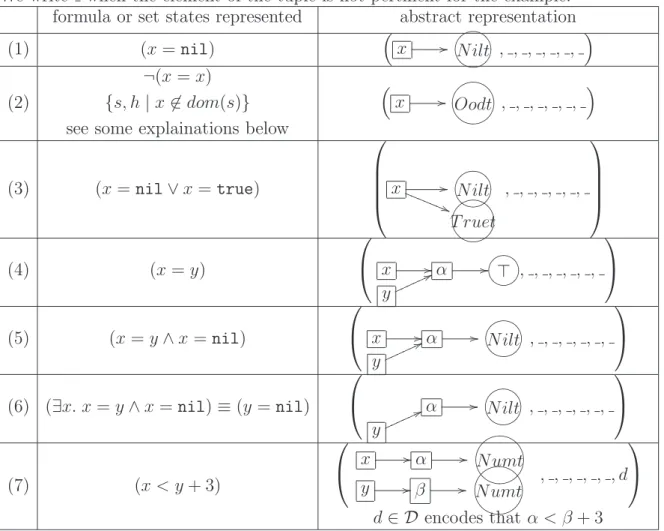
As for the abstract language we designed, the process was the same: we started with a very simple domain, nil or not, then we added graphs that were quite similar to shape graphs. Then, we needed auxiliary variables to say“x = y” and then say “x = nil” but yet not have to re-check which values equal to x when refining the informations about “x” and its aliases: x //α //GFED@ABC⊤
ynnnnn 66n
then x //α // _^]\6 ⊤ nilXYZ[ y 77o o o o o o .
We designed a semantics for the language in the same domain as the model of the logic and itself. This was important in particular for auxiliary variables. First, we wanted that the semantics of a graph would be the intersection of the semantics of its arrows. Secondly, because it permits to write precise proofs about the functions which manipulates elements of the language , the functions that translate formulae while manipulating auxiliary variables are usually presented in papers as part of the implementation and not precisely described. We made this precise and explicit.
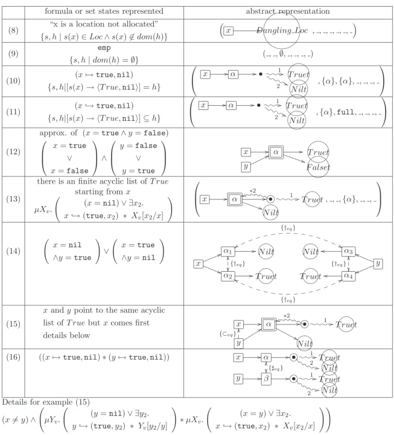
To resemble existing shape graphs, we naturally added summary nodes, nodes which represent several locations, to the graphs to bring some abstraction, but we generalised
them so that they would represent not only multiple locations but they could also represent any kind of values (numerical, boolean, etc.).
At this point, we did not have information about numericals and as a result most of the time, our result would say “the result is this but may be there is a numerical error” while in fact no numerical would be involved or there were no errors of numericals. So, we parametrised the domain by a numerical domain.
We did not want to record sets of graphs, but only one graph with sets of arrows, but this would imply imprecision during the union, so we created a new subdomain which is table-based, which allows us to keep additional information when we want to make a precise union.
Lastly, the arrows of the graphs include separation information.
Since we can express all pre- and post-conditions in our logic with fixpoints, we can already get information about the program by expressing the pre- and post-conditions and then translating them into our abstract language.
The principal place of abstraction comes when translating fixpoints and building sum-mary nodes. This is interesting because it can provide useful information without knowing in advance the form of data structures used by a program.
If we may summarize the main accomplishments of the thesis, these would be:
• adding fixpoints to separation logic, which provides a way to express recursive for-mulae, expressing preconditions for while-loops, and expressing all post-conditions, letting us prove useful properties about the extended logic
• giving a precise semantics of the abstract domain of separation formulae in terms of sets of memory
• designing the abstract language as a partially reduced product of subdomains
• giving a semantics to auxiliary variables and not leaving this as an implementation design question
• combining the domain’s heap analysis with a numerical domain which could be chosen from existing ones (e.g. polyhedra, octogons)
• designing the novel tabular data structure which allows extra precision by using a graph of sets instead of sets of graphs
1.4
Structure of the manuscript
Chapter 2 presents the extension with fixpoints we added to separation logic. It includes the syntax and semantics of the programs we analyse; the syntax, semantics and some properties of the separation logic with fixpoints; the pre- and post-conditions of programs in the extended logic for any formula and any command including while-loops and their proofs.
Chapter 3 presents the abstract language we have designed. It gives some examples, a precise semantics, and some useful operations on the domain like extension, union, merging nodes, stabilization, the function ast created for translating the connective ∗. The chapter gives the translation of formulae of separation logic with fixpoints into elements of the abstract language and their proofs.
Chapter 4 talks about the implementation of the analysis and in particular the data-structures adopted.
In Chapter 5, we gives comparison to related work. The chapter focuses on two active lines of work which have been operating for several years with many people: “smallfoot”, the work from London, which is the most involved with separation logic, and “TVLA”, a well established work for analysing storage structure.
Chapter 2
Separation logic with fixpoints
In this chapter1, we extend the separation logic, presented in the introduction, with fixpoint connectives to define recursive properties and to express the axiomatic semantics of a while statement. We present forward and backward analyses (sp (strongest postcondition), wlp (weakest liberal precondition) expressed for all statements and all formulae.
In Sect. 2.1, we describe the command language we analyze and in Sect. 2.2, we present our logic BIµν. In Sect. 2.3, we provide a backward analysis with BIµν in terms of “weakest liberal preconditions”. We express the wlp for the composition, if−then−else and while commands. In Sect. 2.4, we provide a forward analysis with BIµν in terms of “strongest postconditions”. In Sect. 2.5, we discuss another possibility for adding fixpoints to separation logic and other works proposed afterward.
2.1
Commands and basic domains
We consider a simple “while”-language with Lisp-like expressions for accessing and creating cons cells.
2.1.1
Command syntax
The commands we consider are as follows.
1
most of this chapter has been plublished in13
C ::= x := E | x := E.i | E.i := E′ | x := cons(E1, E2) | dispose(E) | C1; C2 | if E then C1 else C2 | skip | while E do C1 i ::= 1 | 2
E ::= x | n | nil | T rue | F alse | E1 op E2
An expression can denote an integer, an atom, or a heap-location. Here x is a variable in Var, n an integer and op is an operator in (Val × Val) → Val such as + : (Int × Int) → Int, ∨ : (Bool × Bool) → Bool (for Var and Val, see Sect. 2.1.2).
The second and third assignment statements read and update the heap, respectively. The fourth creates a new cons cell in the heap and places a pointer to it in x.
Notice that in our language we do not handle more than one dereferencings in one statement (no x.i.j, no x.i := y.j); this restriction is for simplicity and does not limit the expressivity of the language, requiring merely the addition of intermediate variables.
2.1.2
Semantic domains
Val = Int ∪ Bool ∪ Atoms ∪ Loc S = Var ⇀ Val
H = Loc ⇀ Val × Val
Here, Loc = {l1, l2, ...} is an infinite set of locations, Var = {x, y, ...} is an infinite set of variables, Atoms = {nil, a, ...} is a set of atoms, and ⇀ is for partial functions. We call an element s ∈ S a stack and h ∈ H a heap. We also call the pair (s, h) ∈ S × H a state.
We use dom(h) to denote the domain of definition of a heap h ∈ H, and dom(s) to denote the domain of a stack s ∈ S. Notice that we allow dom(h) to be infinite.
An expression is interpreted as a heap-independent value: JEKs ∈ Val. For example, JxKs = s(x), JnKs = n, JtrueKs = true, JE1+ E2Ks= JE1Ks+ JE2Ks.
Since domain S allows partial functions, J Ks is also partial. Thus JE
1 = E2Ks means JE1Ks and JE2Ks are defined and equal. From here on, when we write a formula of the form · · · JEKs· · · , we are also asserting that JEKs is defined.
JEKs = v x := E, s, h ; [s|x → v], h JEKs= l h(l) = r x := E.i, s, h ; [s|x → πir], h JEKs = l h(l) = r JE′Ks= v′ E.i = E′, s, h ; s, [h|l → (r|i → v′)] l ∈ dom(h) JEKs = l dispose(E), s, h ; s, (h − l) l ∈ Loc l 6∈ dom(h) JE1Ks = v1, JE2Ks = v
2 x := cons(E1, E2), s, h ; [s|x → l], [h|l → hv1, v2i] C1, s, h ; C′, s′, h′ C1; C2, s, h ; C′; C2, s′, h′ C1, s, h ; s′, h′ C1; C2, s, h ; C2, s′, h′ skip, s, h ; s, h JEKs= T rue ifE then C1 elseC2, s, h ; C1, s, h JEKs= F alse ifE then C1 elseC2, s, h ; C2, s, h JEKs = F alse whileE do C, s, h ; s, h JEKs= T rue whileE do C, s, h ; C; while E do C, s, h
Figure 2.1: Operational small-step semantics of the commands
2.1.3
Small-step semantics
The semantics of statements, C, are given small-step semantics defined by the relation ; on configurations. The configurations include triples C, s, h and terminal configurations s, h for s ∈ S and h ∈ H. The rules are given in Fig. 2.1.
In the rules, we use r for elements of Val × Val; πir with i ∈ {1, 2} for the first or second projection; (r|i → v) for the pair like r except that the i’th component is replaced with v; and [s | x → v] for the stack like s except that it maps x to v, (h − l) for h↾dom(h)\{l}.
The location l in the cons case is not specified uniquely, so a new location is chosen non-deterministically.
Let the set of error configurations be: Ω = {C, s, h | ∄K. C, s, h ; K}. We say that:
• “C, s, h is safe” if and only if ∀K. (C, s, h ;∗ K ⇒ K 6∈ Ω)
• “C, s, h is stuck” if and only if C, s, h ∈ Ω
For instance, an error state can be reached by an attempt to dereference nil or an integer. Note also that the semantics allows dangling references, as in stack [x → l] with
empty heap [].
The definition of safety is formulated with partial correctness in mind: with loops, C, s, h could fail to converge to a terminal configuration but not get stuck.
We define the weakest liberal precondition in the operational domain:
Definition 2.1. For ∆ ⊆ S × H , wlpo(∆, C) = {s, h | (C, s, h ;∗ s′, h′ ⇒ s′, h′ ∈ ∆) ∧ C, s, h is safe}
We define the strongest postcondition similarly:
Definition 2.2. spo(∆, C) = {s′, h′ | ∃s, h ∈ ∆. C, s, h ;∗ s′, h′}
2.2
BI
µνIn this section, we present the logic BIµν. It is designed to describe properties of the state. Typically, for analysis it will be used in Hoare triples of the form {P }C{Q} with P and Q formulae of the logic and C a command.
We present in Sect. 2.2.1 the syntax of the logic and in Sect. 2.2.2its formal semantics. In Sect. 2.2.3, we give the definition of a true triple {P }C{Q}. In Sect. 2.2.4, we discuss the additions to separation logic (fixpoints and postponed substitution).
2.2.1
Syntax of formulae
P, Q, R ::= E = E′ Equality | E 7→ E
1, E2 Points to
| false Falsity | P ⇒ Q Classical Imp.
| ∃x.P Existential Quant. | emp Empty Heap | P ∗ Q Spatial Conj. | P →∗ Q Spatial Imp.
| Xv Formula Variable | P [E/x] Postponed Substitution | νXv.P Greatest Fixpoint | µXv.P Least Fixpoint
We have an infinite set of variables, Varv, used for the variables bound by µ and ν and disjoint from the set Var. They range over sets of states, the others (x,y,...) are variables which range over values. For emphasis, uppercase variables subscripted by v are used to define recursive formulae. We use the term “closed” for the usual notion of closure of
variables in Var (closed by ∃ or ∀) and the term “v-closed” for closure of variables in Varv (v-closed by µ or ν).
Our additions to Reynolds and O’Hearn’s separation logic are the fixed-point operators µXv. P and νXv. P and the substitution construction P [E/x].
We can define various other connectives as usual, rather than taking them as primitives: ¬P , P ⇒ false P ∨ Q , (¬P ) ⇒ Q ∀x.P , ¬(∃x.¬P ) true , ¬(false) P ∧ Q , ¬(¬P ∨ ¬Q) E ֒→ a, b , true ∗ (E 7→ a, b) x = E.i , ∃x1, x2. (E ֒→ x1, x2) ∧ (x = xi)
We could have only one fixpoint connective in the syntax, since the usual equivalences, µXv. P ≡ ¬νXv.¬(P {¬Xv/Xv}) and νXv. P ≡ ¬µXv.¬(P {¬Xv/Xv}), hold (proofs in Sect. 2.6.7).
The set F V (P ) of free variables of a formula is defined as usual. The set Var(P ) of variables of a formula is defined as usual with Var(P [E/x]) = Var(P ) ∪ Var(E) ∪ {x}. (see definitions of F V and V ar in Sect. 2.6.1)
2.2.2
Semantics of formulae
The semantics of the logic is given in Fig. 2.2.
We use the following notations in formulating the semantics:
• h♯h′ indicates that the domains of heaps h and h′ are disjoint;
• h · h′ denotes the union of disjoint heaps (i.e., the union of functions with disjoint domains).
We express the semantics of the formulae in an environment ρ mapping formula variables to set of states: ρ : Varv ⇀P(S × H). The semantics of a formula in an environment ρ is the set of states which satisfy it, and is expressed by: J·Kρ : BIµν ⇀P(S × H)
We call JP K the semantics of a formula P in an empty environment JP K = JP K∅. We also define a forcing relation of the form:
JE = E′Kρ = {s, h | JEKs = JE′Ks} JE 7→ E1, E2Kρ = {s, h | dom(h) = {JEKs}
and h(JEKs) = hJE
1Ks, JE2Ksi} JfalseKρ = ∅ JP ⇒ QKρ = ((S × H) \ JP Kρ) ∪ JQKρ J∃x.P Kρ = {s, h | ∃v ∈ Val.[s|x → v], h ∈ JP Kρ} JempKρ = {s, h | h = []} JP ∗ QKρ = {s, h | ∃h0, h1. h0♯h1, h = h0· h1 s, h0 ∈ JP Kρand s, h1 ∈ JQKρ} JP →∗QKρ = {s, h | ∀h′. if h♯h′ and s, h′ ∈ JP Kρ then s, h · h′ ∈ JQKρ} JXvKρ = ρ(Xv) , if Xv ∈ dom(ρ) JµXv . P Kρ = lfp⊆∅λX. JP K[ρ|Xv→X] JνXv . P Kρ = gfp⊆∅λX. JP K[ρ|Xv→X] JP [E/x]Kρ = {s, h | [s | x → JEKs], h ∈ JP Kρ} Figure 2.2: Semantics of BIµν and an equivalence:
P ≡ Q if and only if ∀ρ.(JP Kρ = JQKρ) or (JP Kρand JQKρboth do not exist).
In both cases µ and ν, the X in λX is a fresh variable over sets of elements in S × H which does not already occur in ρ.
Notice that J·Kρ is only a partial function. In definitions above, lfp⊆∅λX. JP K[ρ|Xv→X] (gfp⊆∅λX. JP K[ρ|Xv→X]) is the least fixpoint (greatest fixpoint) of the function λX. JP K[ρ|Xv→X] on the poset hP(S × H), ⊆i, if it exists. Otherwise, JµXv.P Kρ (JνXv.P Kρ) is not defined. For example, this is the case for µXv . (Xv ⇒ false).
The syntactical criterions for formulae with defined semantics (like parity of negation under a fixpoint, etc.) are the usual ones knowing that in terms of monotonicity, →∗ acts like ⇒, ∗ acts like ∧, and [ / ] does not interfere. The fixpoint theory gives us criteria (using Tarski’s fixpoint theorem) for the existence of JP Kρ, but no criteria for nonexistence. Nonetheless, we have these facts:
is monotonic and antitonic.
• JXvKρ exists if and only if Xv ∈ dom(ρ); λX.JXvK[ρ|Yv→X] is monotonic and not anti-tonic.
• If P is Q ⇒ R or Q→∗R, then JP Kρ exists if and only if JQKρ and JRKρ exist; λX.JP K[ρ|Xv→X] is monotonic if and only if λX.JRK[ρ|Xv→X] is monotonic and
λX.JQK[ρ|Xv→X] is antitonic; λX.JP K[ρ|Xv→X] is antitonic if and only if λX.JRK[ρ|Xv→X] is antitonic and λX.JQK[ρ|Xv→X] is monotonic.
• JQ ∗ RKρ exists if and only if JQKρ and JRKρ exist; λX.JQ ∗ RK[ρ|Xv→X] is mono-tonic/antitonic if and only if λX.JRK[ρ|Xv→X] and λX.JQK[ρ|Xv→X] are
monotonic/antitonic.
• If P is ∃x. Q or Q[E/x], then JP Kρexists if and only if JQKρ exists; λX.JP K[ρ|Xv→X] is monotonic/antitonic if and only if λX.JQK[ρ|Xv→X] is monotonic/antitonic.
• If µν ∈ {µ, ν} and if λX.JP K[ρ|Xv→X] exists and is monotonic, then JµνXv. P Kρ exists and λX.JµνXv. P K[ρ|Xv→X] is monotonic and antitonic.
• If µν ∈ {µ, ν} and if λX.JP K[ρ|Xv→X|Yv→Y ] is monotonic/antitonic, and
λY.JP K[ρ|Xv→X|Yv→Y ] exists and is monotonic, then λX.JµνYv. P K[ρ|Xv→X] is mono-tonic/antitonic.
2.2.3
Interpretation of Triples
Hoare triples are of the form {P }C{Q}, where P and Q are assertions in BIµν and C is a command. The interpretation ensures that well-specified commands do not get stuck. (In this, it differs from the usual interpretation of Hoare triples15.)
Definition 2.3. {P }C{Q} is a true triple if and only if ∀s, h, if s, h |= P and F V (Q) ⊆ dom(s), then
• if C, s, h ;∗ s′, h′, then s′, h′ |= Q.
This is a partial correctness interpretation; with looping, it does not guarantee termi-nation. This is the reason for expressing “weakest liberal preconditions” for our backward analysis and not “weakest preconditions”. However, the safety requirement rules out certain runtime errors and, as a result, we do not have that {true}C{true} holds for all commands. For example, {true}x := nil; x.1 := 3{true} is not a true triple.
2.2.4
Fixpoints and postponed substitution
In this section, we discuss our motivations for adding fixpoints and postponed substitution to separation logic. We show that the postponed substitution connective, [ / ], is not classical substitution, { / }, and that the usual variable renaming theorem does not hold for { / }. We develop the needed concepts in a series of vignettes:
First motivation
Our initial motivation for adding fixpoint operators to separation logic came from the habit of the separation logic community of informally defining recursive formulae and using them in proofs of correctness.
Since we have added fixed-point operators to the logic, we can formally and correctly express, for example, that x is a non-cyclic finite linear list as
nclist(x) = µXv. (x = nil) ∨ ∃x1, x2.(isval(x1) ∧ (x 7→ x1, x2 ∗ Xv[x2/x])) and that x is non-cyclic finite or infinite list
nclist(x) = νXv. (x = nil) ∨ ∃x1, x2.(isval(x1) ∧ (x 7→ x1, x2 ∗ Xv[x2/x]))
where isval(x) = (x = true) ∨ (x = false) ∨ (∃n.n = x + 1) In earlier papers16, Reynolds and O’Hearn use the definition,
nclist(x) = (x = nil) ∨ ∃x1, x2.(isval(x1) ∧ (x 7→ x1, x2 ∗ nclist(x2)))
Second motivation
The second motivation was the formulations of the wlp ({ ? }C{P }) and sp ({P }C{ ? }) in the case of while commands, which was not possible earlier. This problem is nontrivial: For separation logic without fixed-points, we might express sp as
sp(P, while E do C) = (lfp|=false λX.sp(X ∧ E = true, C) ∨ P ) ∧ (E = false)
with lfp|=false λX.F (X) defined, if it exists, as a formula P which satisfies:
• P ≡ F (P )
• for any formula Q, (Q ≡ F (Q) implies P |= Q )
where
• Q |= P if and only if JQK ⊆ JP K or JQK and JP K are both not defined; • P ≡ Q if and only if P |= Q and Q |= P .
This implies that during the computation of the sp, each time a while loop occurs, we must find a formula in existing separation logic that was provably the fixpoint, so that we could continue the computation of the sp. In another sense, this “work” could be seen as the “work” of finding the strongest loop invariant in the application of the usual rule for while loop.
Our addition of fixpoints (and the related postponed substitution) allows us to express the sp directly within the logic:
sp(P, while E do C) = (µXv.sp(Xv∧ E = true, C) ∨ P ) ∧ (E = false).
Although the definitions of the wlp and sp for the while loop are simple and elegant, the “work” of finding loop invariants is not skipped, however it is now postponed for when we have a specific proof to undertake. In the following chapters, we will present translations of formulae into an other domain, and we have to find an approximation of the translation
of fixpoints which is precise and not too expensive to compute. The advantage here is that this work of building the translation is done once and for all, then the analysis can be fully automated while the methodology of a proof system and finding loop invariant implies hand work.
[ / ] is not { / }
We use the notation P {E/x} for capture-avoiding syntactical substitution (that is, the usual substitution of variables). Recall that [ / ] is a connective of the logic (called postponed substitution) and is not equivalent to { / }. It might be helpful for the reader to understand [ / ] to look at the formula P [E/x] as (Moggi’s12) call-by-value, let x = E in P .
The distinction between [ / ] and { / } can be viewed in this example, where the command will be stuck in any state that has no value in its stack for y:
{true}x := y{true} is false
This implies that the classical axiom for assignment, {P {y/x}}x := y{P }, is unsound. In other versions of separation logic6, {P {y/x}}x := y{P } was sound, since the definition
of a true triple required F V (C, Q) ⊆ dom(s) and not merely F V (Q) ⊆ dom(s), as here, and also because there was no recursion.
Our definition along with the choice to allow stacks to be partial functions does not require variables of the program to have a default value in the stack and it checks whether a variable has been assigned before we try to access its value. But the addition of fixpoints does not require stacks to be partial functions. (Indeed, if stacks were total functions, then more laws would hold for [ / ], but the latter’s definition would remain different from { / }’s.)
Unfolding
As usual, we have µXv.P ≡ P {µXv.P/Xv} and νXv.P ≡ P {νXv.P/Xv}
{/}: No variable renaming
Surprisingly, we have ∃y.P 6≡ ∃z.P {z/y} with z 6∈ Var(P ) (when y 6= z). Here are two counterexamples, which expose the difficulties:
Counterexample 1:
JνXv.y = 3 ∧ ∃y.(Xv∧ y = 5)K 6≡ JνXv.y = 3 ∧ ∃z.(Xv∧ z = 5)K
The left-hand side denotes the empty set, while the right-hand side denotes Jy = 3K. Here are the detailed calculations:
JνXv.y = 3 ∧ ∃y.(Xv∧y= 5)K∅
= gfp⊆∅λY. Jy = 3 ∧ ∃y.(Xv∧y= 5)K[Xv→Y ]
= gfp⊆∅λY. Jy = 3K[Xv→Y ]∩ J∃y.(Xv∧y = 5)K[Xv→Y ]
= gfp⊆∅λY. {s, h | s(y) = 3} ∩ {s, h | ∃v.[s |y → v], h ∈ JXv ∧y = 5K[Xv→Y ]} = gfp⊆∅λY. {s, h | s(y) = 3} ∩ {s, h | ∃v.[s |y → v], h ∈ Y ∧ [s |y → v](y) = 5} = gfp⊆∅λY. {s, h | s(y) = 3} ∩ {s, h | [s |y→ 5], h ∈ Y }
= ∅
JνXv.y = 3 ∧ ∃z.(Xv∧z = 5)K∅
= gfp⊆∅λY. Jy = 3 ∧ ∃z.(Xv∧z = 5)K[Xv→Y ]
= gfp⊆∅λY. Jy = 3K[Xv→Y ]∩ J∃z.(Xv ∧z= 5)K[Xv→Y ]
= gfp⊆∅λY. {s, h | s(y) = 3} ∩ {s, h | ∃v.[s |z → v], h ∈ JXv ∧z= 5K[Xv→Y ]} = gfp⊆∅λY. {s, h | s(y) = 3} ∩ {s, h | ∃v.[s |z → v], h ∈ Y ∧ [s |z→ v](z) = 5} = gfp⊆∅λY. {s, h | s(y) = 3} ∩ {s, h | [s |z → 5], h ∈ Y }
= {s, h | s(y) = 3}
Here is some intuition: For the left-hand side, y = 3 says that all the states defined by the assertion must bind y to 3, and “∃y.Xv ∧ y = 5” says that for all those states defined by the assertion, we can bind y such that it satisfies y = 5, even as it satisfies y = 3, due to the recursion, which is impossible, so we have ∅ as the denotation.
For the right-hand side, y = 3 asserts again that y binds to 3, and ∃z.Xv∧ z = 5 says that for all states in the assertion’s denotation, we bind 5 to z, which is indeed possible, so we have Jy = 3K as the denotation of the assertion.
Counterexample 1 shows that variable renaming has a special behavior when applied to a formula which is not v-closed.
Counterexample 2:
J∃y.νXv.y = 3 ∧ ∃y.(Xv ∧ y = 5)K 6≡ J∃z.νXv.z = 3 ∧ ∃y.(Xv∧ y = 5)K The left-hand side denotes the empty set, while the right-hand side denotes S × H.
To see this, note that the left-hand side’s semantics is essentially the same as its coun-terpart in the first counterexample. As for the right-hand side, if we apply the semantics of the right-hand side of the first counterexample, we see that JνXv.z = 3 ∧ ∃y.(Xv ∧ y = 5)K = Jz = 3K, signifying that all the states are such that we bind 5 to z. So, we have S × H as the denotation of the right-hand side.
Counterexample 2 shows that variables occurring free in the bodies of fixed-point for-mulae are subject to dynamic binding with respect to unrolling the recursive forfor-mulae via postponed substitution.
Full substitution
The previous counterexample 2 leads to the definition of a new substitution:
Definition 2.4. Let {[ / ]} be a full syntactical variable substitution: P {[z/y]} is P in which all y are replaced by z wherever they occur, for example:
(∃y.P ){[z/y]} , ∃z.(P {[z/y]}), (P [E/x]){[z/y]} , (P {[z/y]})[E{z/y}/x{z/y}]
The variable renaming theorem for BIµν
We define class(z, s, h) as the set of states containing the state, s, h, and all other states identical to s, h except for z:
Definition 2.5. class(z, s, h) = {s′, h | for all v ∈ V al, [s′ | z → v] = [s | z → v]}
Alternatively, we can say that class(z, s, h) is that set which satisfies:
• ∀v.[s | z → v], h ∈ class(z, s, h)
Definition 2.6. For z ∈ V ar, X ∈ P(S × H), define
nodep(z, X) , T rue iff ∀s, h ∈ X.class(z, s, h) ⊆ X
We extend this definition to environments as well:
nodep(z, ρ) , T rue iff (∀Xv ∈ dom(ρ).nodep(z, ρ(Xv))
Proposition 2.7. If nodep(z, ρ), F Vv(P ) ⊆ dom(ρ), z 6∈ F V (P ) and JP Kρ exists, then nodep(z, JP Kρ)
The proof is found in Sect. 2.6.2.
The idea is, if P is v-closed and z does not occur free in P , then ∀v. (s, h ∈ JP K iff [s | z → v], h ∈ JP K). Yet another phrasing goes, if z does not occur free in a v-closed formula, then the set of states satisfying the formula does not have any particular values for z.
Now, let • s• y,z , " [s | y → s(z)] if z ∈ dom(s) s if z 6∈ dom(s) • ρ•
y,z , [∀Xv ∈ dom(ρ). Xv → {s, h | s•y,z, h ∈ ρ(Xv)}]
Proposition 2.8. If nodep(z, ρ) and z 6∈ V ar(P ), then JP {[z/y]}Kρ•
y,z = {s, h | s • y,z, h ∈ JP Kρ}
Theorem 2.9. If P is v-closed, z 6∈ V ar(P ) and y 6∈ F V (P ), then P ≡ P {[z/y]}. In particular, ∃y.P ≡ ∃z.(P {[z/y]}).
You can see proofs and details in Sect. 2.6.3. Equivalences on [ / ]
For proofs see Sect. 2.6.8.
We define is(E) , E = E, which is just a formula ensuring that E has a value in the current state. If we had chosen that stacks were only total functions, is(E) would always be equivalent to true and there would be more simplifications. We have these facts: