1
Statistical Properties of Dayside Subauroral Proton
2Flashes observed with IMAGE-FUV.
3B. Hubert
(1), J.C. Gérard
(1), S. B. Mende
(2), and S. A. Fuselier
(3).
4
(1) Laboratoire de Physique Atmosphérique et Planétaire, Université de Liège, Belgium. 5
(2) Space Sciences Laboratory, University of California, Berkeley, California, USA. 6
(3) Lockheed Martin Advanced Technology Center, Palo Alto, California, USA. 7
Abstract.
1
The SI12 instrument of the FUV experiment onboard the IMAGE satellite is specifically 2
devoted to the observation of the proton aurora. Transient subauroral proton aurora was 3
detected with SI12 in response to a solar wind dynamic pressure increase. These Dayside 4
Subauroral Proton Flashes (DSPF's) take place on field lines of L-Shell as low as 4, and 5
possibly result of an increase of EMIC growth rate instability due to the compression of the 6
dayside magnetosphere by the increased solar wind dynamic pressure. In this study, a set of 7
75 DSPF's observed with SI12 related with a solar wind dynamic pressure increase is studied. 8
Statistical distributions of relevant quantitative and morphologic indicators of the DSPF's 9
properties are computed. Correlations between these indicators and the solar wind properties 10
are also studied. It is found that the solar wind dynamic pressure is the key parameter 11
controlling the DSPF maximum power, maximum flux, magnetic latitude and extent in MLT. 12
Also, DSPF's occur preferentially in the afternoon sector, where the plasma temperature 13
anisotropy is higher, so that the EMIC instability threshold is more easily exceeded. 14
Moreover, no correlation is found between the DSPF's characteristic decay time and the solar 15
wind properties, suggesting that this parameter is internally controlled by the properties of the 16
magnetospheric plasma. In this dataset, no correlation is found relating the IMF and the 17 DSPF properties. 18 19
1. Introduction
20Since the launch of the IMAGE spacecraft in March 2000 [Burch 2000], the 21
Spectrographic Imager at 121,8 nm (SI12) instrument of the IMAGE-FUV experiment 22
[Mende et al., 2000 a, b] has been widely used to image the Earth's proton aurora on a global 23
scale. This experiment also includes two other far ultraviolet imagers, the Wideband Imaging 24
Camera (WIC) and the Spectrographic Imager at 135.6 nm (SI13), providing images of the 25
N2-LBH band and OI-135.6 nm emissions respectively. These two emissions are mainly
1
excited by electron impact, but they are also present in the proton aurora [Hubert et al., 2
2001]. 3
Recently, a new transient dayside subauroral feature was observed by Hubert et al. 4
[2003]. These Dayside Subauroral Proton Flashes (DSPF) are connected to an increase of the 5
solar wind dynamic pressure compressing the dayside magnetosphere. A comparison of the 6
SI12, SI13 and WIC observations revealed that DSPF's are due to proton precipitations. 7
Using in situ particles measurement, Zhang et al. [2003] confirmed that the precipitation 8
causing these features is mostly composed of energetic protons. As shown by Hubert et al. 9
[2003], the field lines threading the observed DSPF's map in the equatorial plane at distances 10
as low as 4 RE. It must be noted that DSPF's are possibly related with the subauroral
11
emissions previously reported by Liou et al. [2002] using POLAR-UVI data, without the 12
ability to distinguish between electron and proton precipitations. 13
Fuselier et al. [2004] described a mechanism responsible for the proton precipitation 14
in Dayside Subauroral Proton Flashes (DSPF): following compression of the dayside 15
magnetosphere by the increased solar wind dynamic pressure, the Electromagnetic Ion 16
Cyclotron (EMIC) growth rate turns unstable. This instability diverts protons into the loss 17
cone along low L-shell field lines. Indeed, the stable/unstable issue of the EMIC growth rate 18
is controlled by the plasma parameter and the temperature anisotropy. Balance of the 19
competing effects leads to an instability region corresponding to subauroral latitudes, 20
eventually leading to a gap separating the auroral oval and the proton flash, as observed by 21
Hubert et al. [2003]. 22
In this paper, we use a set of 75 Dayside Subauroral Proton Flashes observed with 23
IMAGE-FUV in order to determine their statistical properties. This set of events was built 24
following a detailed inspection of the IMAGE-FUV dataset and of the solar wind properties 25
measured with the ACE, WIND and GEOTAIL spacecrafts. In the present study, events were 1
selected when a transient proton precipitation is seen in the SI12 images and is related with 2
an increase of the solar wind dynamic pressure obtained from the ACE, GEOTAIL and/or 3
WIND satellites (DSPF’s appearing in the absence of a pressure increase are not included in 4
this dataset and will be the subject of further studies). Not only CME-induced events were 5
included in the set, but also weak proton flashes related with a moderate solar wind dynamic 6
pressure increase. 7
2. Power and decay time.
8
2.1. Statistical distribution 9
The power precipitated into each proton flash was determined using the SI12 10
observations. Figure 1 presents the SI12 images obtained for the DSPF observed on 11
November 8 2000 at 0614 UT, as already presented in Hubert et al. [2003] and reproduced 12
here for convenience. The DSPF clearly appears on the dayside, well centered on the noon 13
sector, and detached from the auroral oval. The power of the proton precipitation of the flash 14
observed on November 8 2000 is calculated for each SI12 image [Hubert et al., 2002]. It is 15
plotted versus time in Figure 2, with t = 0 corresponding to 0612 UT. The sudden increase of 16
the power is conspicuous, and takes place on a time scale shorter than 2 minutes, i.e. less than 17
the time resolution of the SI12 observations. The maximum power obtained from the SI12 18
data is 0.53 GW. After reaching its maximum value, the power decreases roughly 19
exponentially, with a characteristic decay time of ~2 minutes. In this case, a second minor 20
peak is observed some 12 minutes after the main peak. Considering that the solar wind 21
dynamic pressure related with this event [Hubert et al.,2003], as deduced from the ACE 22
satellite measurements, presents two successive ramps separated by ~12 minutes, it may be 23
speculated that the main peak of the subauroral proton flash is related to the first pressure 24
increase, whereas the second dynamic pressure increase, though much more spectacular than 25
the first one, is responsible for the minor peak of the observed DSPF, the dayside flux tubes 1
having already been emptied of a significant part of their proton population. 2
Considering this example, it is natural to define two parameters describing the 3
properties of a DSPF: the maximum power reached during the event, and its characteristic 4
exponential decay time. The maximum power is an indicator of the brightness of the flash as 5
a whole. The actual peak value can be larger, as the time resolution of 2 minutes could easily 6
miss the peak value. Figure 3 shows the distribution of the maximum proton power for our 7
set of selected DSPF's. This asymmetric distribution has an average value of 0.24 0.003 8
GW, the standard deviation of the distribution being = 0.26 GW. The relation between the 9
amplitude of the solar wind pressure pulse and the power of the proton precipitation of the 10
resulting Dayside Subauroral Proton Flash will be investigated later. Figure 4 presents the 11
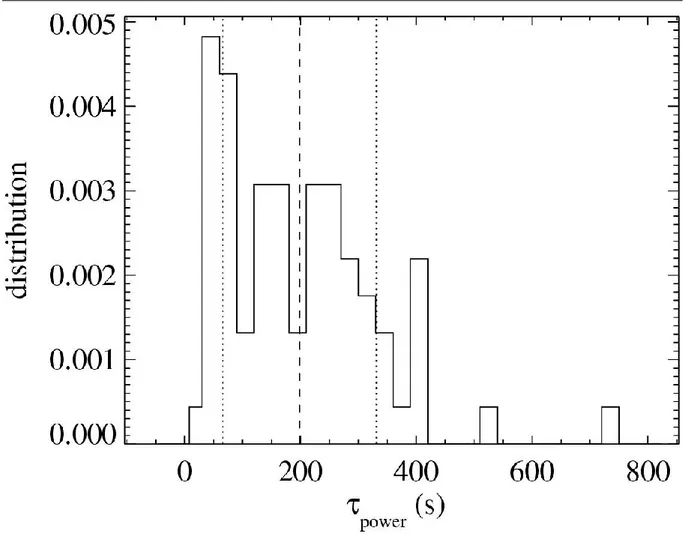
distribution of the DSPF characteristic decay time obtained by fitting an exponential function 12
to the proton power curve of each event. It is, on average ~199 15 s. Anticipating on the 13
following section, we note that no correlation could be found between the determined decay 14
time and the solar wind properties. This suggests that the decay time is internally controlled 15
by the properties of the magnetosphere. It must also be stressed that decay times smaller than 16
2 minutes are poorly estimated, because the FUV experiment has a time resolution of 2 17
minutes. 18
2.2 Correlation with the solar wind parameters 19
In the present study, the criterion used to asses the correlation or uncorrelation 20
between two parameters is the uncorrelation criterion of Fisher [Press et al., 1989]. If r is the 21
linear correlation coefficient, Z is defined as 22
11 rr ln 2 1 Z (1) 23Let also uβ be defined such that there is a probability for a Gaussian random variable of 1
mean 0 and standard deviation 1 to be smaller than uβ. Fisher's criterion then states that two 2
variables are uncorrelated under a level of confidence when the relation 3 3 n u Z 3 n u 2 α 1 2 α 1 (2) 4
is verified, where n is the number of observations (n 10). We will thus accept the 5
hypothesis that two variables are correlated under the level of confidence 1- when the 6
relation (2) is not verified, that is when 7 3 n u Z 2 α 1 (3) 8
The larger | r |, the larger | Z |, so that one need | r | to be sufficiently large to accept 9
the correlation hypothesis. As u increases with , it is clear that the smaller , the more
10
constraining the constraint of relation (2) being not fulfilled. As a consequence, an increase 11
of the level of confidence 1- strengthens the requirements for Fisher's correlation test, as 12
expected. If we select a confidence level of 0.9, i.e. = 0.1, it follows that u 1.65
2 α
1 , so that
13
for n=75, the critical value for Z discriminating between uncorrelated and correlated variables 14
corresponds to r ~ 0.2 only. 15
For those DSPF’s apparently driven by a solar wind dynamics pressure increase, it is 16
expected that the brightness, and hence the power of the observed DSPF's is related in some 17
way to the solar wind dynamic pressure Pdyn (assuming that the protons content of the
18
disturbed flux tubes is sufficiently high). The time interval of the solar wind data related with 19
an observed DSPF was individually identified for each case, accounting for the solar wind 20
propagation time from the satellite to the front of the magnetosphere. Several quantities can 21
then be defined to describe the dynamic pressure pulse (even in the case of a weak pulse) that 1
is responsible for the DSPF proton precipitation. First, the maximum value reached by the 2
temporal derivative of Pdyn ,
max
dt
dP is an indicator of the strength of the dynamic pressure 3
increase. However, this maximum value is only a punctual indicator, and a second indicator 4
can be considered for the pressure ramp as a whole: the average temporal derivative of Pdyn ,
5
dt
dP computed on the time interval starting right prior to the pressure increase and ending
6
when the dynamics pressure reaches its maximum. Even if the average temporal derivative of 7
Pdyn is large, the pressure increase may take place during such a short period of time that the
8
pressure shock would actually be of small amplitude. Consequently, both the maximum 9
pressure reached during the event, Pmax , and the solar wind dynamic pressure variation P,
10
i.e. the solar wind dynamic pressure increase across the event, also appear as valuable 11
indicators of the properties of the solar wind pressure pulse. 12
As already mentioned in a previous paragraph, no correlation could be found between 13
the characteristic decay time of the power of the Dayside Subauroral Proton Flashes and the 14
solar wind properties (Figure 5). Correlation coefficients of –0.024, -0.037, -0.045 and 15
–0.094 were found with
max
dt dP ,
dt
dP, P and P
max respectively. The absence of correlation
16
suggests that this parameter is controlled by the internal properties of the magnetosphere, 17
which integrates over the longer term history of the system. 18
Figure 6a presents the correlation between the proton flash maximum power Wp-max
19
and
max
dt
dP . With a correlation coefficient of 0.78, larger than the threshold value of 0.2 20
determined before, these two quantities are significantly correlated. The outlier at 21
Wp-max~1.8 GW is a reliable point representing an event characterized by a large solar wind
22
velocity of ~900 km/s. This point strongly constrains the regression. If ignored, the 23
correlation coefficient is r = 0.54, still leading to the same conclusion regarding the 1
correlation. The relations between Wp-max and the average temporal derivative
dt dP, the
2
pressure variation P and the maximum solar wind dynamic pressure Pmax are shown as well
3
and all present a statistically significant correlation. As the four correlation coefficients are 4
roughly equal to each other, the four indicators proposed here to quantify the strength of the 5
solar wind pressure pulse appear as equivalent. These correlations simply indicate that the 6
stronger the solar wind disturbance, the stronger the response in power of the proton 7
precipitation to the solar wind pressure pulse. However, the large dispersion of the data 8
indicates the solar wind dynamic pressure is not the only parameter controlling the strength 9
of the proton precipitation. One can indeed expect that the state of the magnetosphere also 10
constrains the auroral response to the pressure increase. In addition, a correlation does not 11
necessarily imply a causal link. From a physical standpoint, inferring such a causal link at the 12
light of a correlation study only makes sense if an underlying precipitation mechanism driven 13
by the pressure increase can be identified. Such a mechanism diverting protons into the loss 14
cone was briefly proposed by Hubert et al. [2003] and thoroughly analyzed by Fuselier et al. 15
[2004]. Two possible behaviors of the observed DSPF's may explain the dependence of 16
Wp-max on the solar wind dynamic pressure: the precipitated proton flux can be stronger, or
17
the spatial extent of the DSPF could be larger (or both), when the solar wind pressure 18
increase is stronger. We discuss these points in the next paragraphs. 19
3. Proton flux.
20
The maximum value reached by the proton flux during the event, Fmax, can also be
21
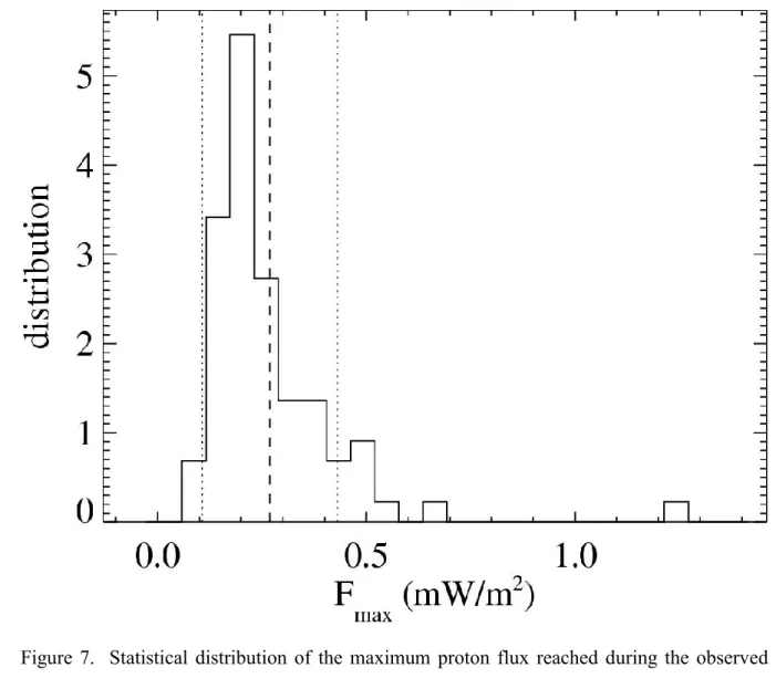
considered as an indicator of the brightness of the observed DSPF's. This indicator works at 22
the local scale, in contrast with Wp-max that concerns the global scale. Figure 7 presents the
23
statistical distribution of Fmax. The predominance of rather weak events also appears in the
24
asymmetry of the distribution. The average value is 0.27 0.02 mW/m2. 25
Figure 8 presents the correlation of Fmax with max dt dP (a), dt dP (b), P (c) and P max (d). 1
The correlation coefficients are 0.69, 0.66, 0.67 and 0.69 respectively. These results indicate 2
that larger solar wind pressure pulses result in larger proton precipitation. This can be 3
understood in terms of the mechanism proposed by Fuselier et al. [2004]: the stronger the 4
compression of the dayside magnetosphere, the larger the disturbance of the inner 5
geomagnetic field at dayside. Thus the EMIC growth rate will be larger and will turn more 6 unstable. 7
4. Morphological parameters.
8 4.1. Statistical distributions. 9We now focus on the magnetic latitude (MLAT) and the extent in magnetic local time 10
(MLT) of the proton precipitation of the observed DSPF events. A relation between these 11
morphological parameters and the solar wind variation triggering the DSPF is expected. The 12
MLAT location of the observed DSPF is determined by the field lines along which the 13
disturbance efficiently fills the loss cone, by establishing an unstable EMIC growth rate for 14
example. The MLT extent of the DSPF quantifies the size of the magnetospheric region 15
compressed by the solar wind pressure increase. 16
Figure 9 shows the distribution of the MLAT of the center of the dayside subauroral 17
proton flash, defined as the average MLAT weighted by the proton flux. The distribution of 18
MLAT is centered on 68° 0.3°, with a standard deviation of 3°. About 8% of the observed 19
DSPF's occur at an average MLAT less than 65°. Figure 10 presents the distribution of the 20
average magnetic local time (MLT) of the observed DSPF's and their MLT extent (MLT). 21
The DSPF's are seen preferentially in the afternoon sector (MLT = 1258 0009 MLT on 22
average). This may be related with the asymmetry of the temperature anisotropy observed in 23
the dayside magnetosphere, this anisotropy being higher in the afternoon sector [Thomsen M. 24
F., personnal communication, Anderson et al., 1996]. A larger temperature anisotropy favors 1
the EMIC instability thought to be responsible for the proton precipitation in DSPF's 2
[Fuselier et al., 2004]. The average value of MLT is 3.6 0.18 MLT hours, the standard 3
deviation of its distribution is 1.3 MLT hour. 4
4.2. Correlation with solar wind parameters. 5
As shown in Figure 11, the magnetic latitude of the observed DSPF's appears 6
statistically anticorrelated with the solar wind dynamic pressure variation and maximum 7
value. The correlation coefficients with
max
dt dP ,
dt
dP , P and P
max are –0.45, -0.37, -0.47 and
8
-0.50 respectively. This tendency is weakly pronounced, as the low correlation coefficients 9
suggest, but it is nevertheless compatible with the EMIC mechanism proposed by Fuselier et 10
al. [2004]: a stronger compression of the magnetosphere results in stronger disturbances at 11
deeper L-shell, causing the instability threshold to be overcome on field lines threading 12
regions of lower magnetic latitude. 13
Figure 12 examines the correlation of the MLT extent of the DSPF's and
max dt dP , dt dP, 14
P and Pmax. The correlation coefficients are 0.22, 0.13, 0.22 and 0.17 respectively. Only
15
correlation coefficients larger than 0.2 can be considered as representing a correlation at a 16
level of confidence of 0.9, as was discussed before. Nevertheless, rejecting the outlier having 17 s nPa/ 39 . 0 dt dP max
from the dataset leads to correlation coefficients of 0.32, 0.16, 0.30 and 18
0.23 respectively, so that the correlation hypothesis can be considered with all variables but 19
dt
dP, this case being disturbed by a second outlier at dt
dP 0.95 nPa/s. The correlation of the
20
MLT extent with the solar wind dynamic pressure indicators of the pressure pulse is not sharp 21
at all. The morphology of the proton precipitation in DSPF's can also depend on other solar 22
wind parameters, such as the orientation of the shock normal etc., but also on the state of the 23
disturbed flux tubes, if we refer to the EMIC-based precipitation mechanism of Fuselier et al. 1
[2004]. The magnitude of the solar wind pressure pulse is probably not the factor controlling 2
the MLT extent of the DSPF precipitation. 3
5. Influence of the IMF.
4
No correlation could be found between the IMF components and the morphological 5
and quantitative properties of the observed DSPF's. Most of the correlation coefficients of the 6
DSPF's properties and the IMF components were close to 0.2, and generally lower. The 7
visual inspection of the few cases of correlation revealed that outliers were responsible for 8
the alleged correlation. We also tested the correlation between the IMF components averaged 9
over a few minutes to an hour before the DSPF events and found no correlation, so that no 10
preconditioning of the magnetosphere by the IMF could be established based on our dataset. 11
Sonnerup and Cahill [1967] proposed a method to determine the shock normal based on IMF 12
measurements. We conducted a study to determine the possible relation between the shock 13
normal orientation and the central MLT of the observed DSPF’s. This study revealed 14
inconclusive, but it must be noted that the concept of shock normal is loosely defined in the 15
case of a small pressure increase. 16
6. Discussion.
17
Figure 6 suggests a correlation between the proton flash power (indicator of the global 18
brightness of the observed dayside subauroral proton flashes) and the four dynamic pressure 19
indicators used here, despite the scatter of the data. The EMIC mechanism is compatible with 20
such a correlation, and the causal relation between the pressure increase and the proton 21
flashes is demonstrated, as expected. A similar conclusion can be drawn concerning Fmax
22
(local indicator of the DSPF brightness) and its correlation with the solar wind dynamic 23
pressure variation. Figure 8 shows the tendency: a stronger pressure increase leads to a more 24
intense proton precipitation at dayside subauroral latitudes, with nevertheless some scatter of 25
the data. Both the quantitative statistical criterion and the physical mechanism proposed to 1
explain the proton precipitation are compatible with the conclusion of a correlation between 2
the intensity of the pressure increase and the peak proton flux of the proton flash. The 3
dispersion of the data is actually not surprising, as the compression of the dayside 4
magnetosphere is not the only parameter controlling the precipitation mechanism. The 5
variability of the plasma properties, in particular the magnitude of the trapped particle 6
reservoir inside of the magnetosphere, probably play a role on the amount of precipitated 7
proton flux and power. 8
The correlation between the magnetic latitude of the observed DSPF's and the solar 9
wind dynamic pressure variation also suffers a large scatter of the data, as shown in Figure 10
11. Visual inspection of the plots raises doubts concerning the relation between
dt dP and
11
MLAT (Figure 11 b). Nevertheless, the tendency remains apparent for the three other 12
pressure indicators. Actually, a strict causal link is not expected between MLAT and the solar 13
wind dynamic pressure increase, for the location of the proton precipitation is directly related 14
with the field lines mapping to the region where the magnetospheric plasma has the required 15
properties to allow the EMIC growth rate to turn unstable. The morphological properties of 16
the proton flashes are thus expected to be only partly related with the solar wind dynamic 17
pressure increase. The correlations found in this study, though low in the absolute sense, may 18
be significant considering the complex mechanism relating the Pdyn increase and the final
19
proton precipitation. 20
The lack of correlation of the characteristic decay time of the observed DSPF's and 21
the solar wind properties suggests an internal magnetospheric control of the decay time. The 22
absence of correlation between the observed proton flashes and the IMF is actually not 23
unexpected considering that the precipitation mechanism is not directly related to a 24
reconnection process. 25
The dataset presented in this study only includes cases of DSPF's observed in 1
conjunction with a solar wind dynamic pressure increase. In addition, 47 weak DSPF cases 2
were also found that developed in the absence of a solar wind dynamic pressure increase. 3
These cases are not in contradiction with the causal link between the solar wind pressure and 4
the subauroral proton precipitations, if one admits that any disturbance able to modify the 5
EMIC growth rate up to the instability threshold can generate a dayside subauroral proton 6
flash. We thus suspect that there exists at least one process other than dynamic pressure 7
pulses able to trigger a DSPF precipitation. One such possibility is a directional discontinuity 8
[Burlaga, 1971] causing a sudden change in the normal direction, so that, at the dayside 9
magnetopause, local dynamic pressure variations generate local disturbances propagating to 10
the inner magnetosphere and trigger subauroral proton precipitation. 11
7. Conclusions.
12
In this study, we investigated the statistical morphology and the relation between the 13
Dayside Subauroral Proton Flash phenomenon and the solar wind properties. A solar wind 14
dynamic pressure increase is a driver able to trigger a DSPF, the intensity of which is 15
dependent on the intensity of solar wind dynamic pressure increase, both at the global and 16
local scales. This parameter also partly controls the morphology of the flash, its magnetic 17
latitude and magnetic local time extent being weakly correlated with the magnitude of the 18
pressure increase. The IMF does not appear as a factor controlling the precipitation 19
mechanism, excluding the possibility of a mechanism dependent on a reconnection process 20
between the magnetospheric field and the IMF. The characteristic decay time of the DSPF's 21
does not depend on the solar wind conditions. We thus speculate that the decay time is 22
internally controlled by the properties of the plasma of the inner magnetosphere. The dataset 23
presented here all appear compatible with the mechanism based on the EMIC growth rate 24
proposed by Fuselier et al. [2004]. Other triggering mechanisms than a solar wind dynamic 25
pressure increase must also be considered, as DSPF's were also observed in the absence of 1
such a pressure increase. 2
3 4
Acknowledgements. The success of the IMAGE mission is a tribute to the many dedicated 5
scientists and engineers that have worked and continue to work on the project. The PI for the 6
mission is Dr. J. L. Burch. Jean-Claude Gérard and Benoît Hubert are supported by the 7
Belgian National Fund for Scientific Research (FNRS). This work was funded by the 8
PRODEX program of the European Space Agency (ESA) and the Fund for Collective and 9
Fundamental Research (FRFC grant 01-2.4569.01). Research at Lockheed Martin was 10
supported by the IMAGE data analysis program through subcontract from the University of 11
California, Berkeley. The IMAGE-FUV investigation was supported by NASA through 12
SWRI subcontract number 83820 at the University of California, Berkeley, contract NAS5-13
96020. ACE level 2 data were provided by N.F. Ness (MFI) and D. J. McComas 14
(SWEPAM), and the ACE Science Center. GEOTAIL data (L. Frank, U. Iowa) and WIND 15
data (R. Lepping, NASA/GSFC) were obtained through the CDAweb site. 16
17
References.
18
Anderson, B. J., Denton R. E., Ho G., Hamilton D. C., Fuselier S. A., and Strangeway R. J., 19
Observational test of local proton cyclotron instability in the Earth’s magnetosphere, J. 20
Geophys. Res., 101, 21527, 1996. 21
Burch, J.L., IMAGE Mission overview, Space Science Reviews, 91, 1, 2000 22
Burlaga, L. F., Nature and origin of directional discontinuities in the solar wind, J. Geophys. 23
Res., 76, 4360, 1971. 24
Fuselier, S. A., , S. P. Gary, M. F. Thomsen, E. S. Claflin, B. Hubert, B. R. Sandel, and T. 25
Immel, Generation of Transient Dayside Sub-Auroral Proton Precipitation, J. Geophys. 26
Res., 109, A1227, doi:10.1029/2004JA010393 , 2004. 27
Mende, S.B., H. Heetderks, H.U. Frey, M. Lampton, S.P. Geller, S. Habraken, E. Renotte, C. 28
Jamar, P. Rochus, J. Spann, S.A. Fuselier, J.C. Gérard, G.R. Gladstone, S. Murphree, 1
and L. Cogger, Far ultraviolet imaging from the IMAGE spacecraft: 1. System design, 2
Space Science Reviews, 91, 243, 2000a. 3
Mende, S.B., H. Heetderks, H.U. Frey, J.M. Stock, M. Lampton, S. Geller, R. Abiad, O. 4
Siegmund, S. Habraken, E. Renotte, C. Jamar, P. Rochus, J.C. Gérard, R. Sigler, and H. 5
Lauche, Far ultraviolet imaging from the IMAGE spacecraft : 3. Spectral imaging of 6
Lyman alpha and OI 135.6 nm, Space Science Reviews, 91, 287, 2000b. 7
Hubert, B., J.-C. Gérard, D. V. Bisikalo, V. I. Shematovich, and S. C. Solomon, The role of 8
proton precipitation in the excitation of auroral FUV emissions, J. Geophys. Res., 106, 9
21475, 2001. 10
Hubert, B., J.C. Gérard, D.S. Evans, M. Meurant, S.B. Mende, H.U. Frey, and T.J. Immel, 11
Total electron and proton energy input during auroral substorms: Remote sensing with 12
IMAGE-FUV, J. Geophys. Res., 107, doi: 10.1029/2001JA009229, 2002 13
Hubert, B., J. C. Gérard, S.A. Fuselier, and S. B. Mende, Observation of dayside subauroral 14
proton flashes with the IMAGE-FUV imagers, Geophys. Res. Lett., 30, doi: 15
10.1029/2002GL016464, 2003 16
Liou, K., C.-C. Wu, R. P. Lepping, P. T. Newell, and C.-I. Meng, Midday sub-auroral 17
patches (MSPs) associated with interplanetary shocks, Geophys. Res. Lett., 29, 1771, 18
doi:10.1029/2001GL014182, 2002 19
Press, W. H., B. P. Flannery, S. A. Teukolsky, and W. T. Vetterling, Numerical recip es, the 20
art of scientific computing, FORTRAN version, Cambridge University Press, New York, 21
1989. 22
Sonnerup, B. U. Ö, and L. J. Cahill, Jr., Magnetopause structure and attitude from Explorer 23
12 observations, J. Geophys. Res., 72, 171, 1967. 24
Zhang, Y., L. J. Paxton, T. J. Immel, H. U. Frey, and S. B. Mende, Sudden solar wind 25
dynamic pressure enhancements and dayside detached auroras: IMAGE and DMSP 26
observations, J. Geophys. Res., 108, doi:10.1029/2002JA009355, 2003. 27
28 29
1
Figure 1. SI12 counts remapped in geomagnetic coordinates showing the subauroral proton 2
flash of November 8 2000 at 0614 UT. The background has been removed. Concentric 3
yellow circles are 10° MLAT apart, noon is at the top of each picture (MLT=12). 4
5 6
1
Figure 2. Proton power deduced from the SI12 observations of the Dayside Subauroral 2
Proton Flash that occurred on November 8 2000 at 0614 UT, versus time. The time=0 mark 3
corresponds to 0612 UT. 4
5 6
1
Figure 3. Distribution function of the maximum power reached during the observed DSPF's. 2
The vertical dashed line represents the average value (m=0.24 GW), the vertical dotted lines 3
are the average plus/minus one standard deviation (=0.26 GW). The uncertainty on m is 4
thus ~.003 GW, that is ~13%. 5
6 7
1
Figure 4. Distribution function of the characteristic decay time of the observed DSPF's. The 2
average value is m=199 15 s, and the standard deviation of the distribution is =132 s. The 3
vertical dashed line represents m, the vertical dotted lines represent m . 4
5 6
1 2 3 4
Figure 5. Correlation between the decay time of the proton power of the observed DSPF's 5
and the corresponding maximum value of the temporal derivative of the solar wind dynamic 6
pressure (a), the average value of the derivative (b), the solar wind dynamic pressure 7
variation (c) and the maximum value of Pdyn (d) , deduced from solar wind data of the ACE,
8
WIND and GEOTAIL satellites. Each diamond represents an event, the solid line is a linear 9
best fit to the observations. All four correlation coefficients are smaller than the threshold 10
value of 0.2, so that the decay time is not correlated with these four quantities. 11
12 13
1
2
3
Figure 6. Correlation between the maximum power reached during the observed DSPF's and 4
the corresponding maximum value of the temporal derivative of the solar wind dynamic 5
pressure (a), the average value of the derivative (b), the solar wind dynamic pressure 6
variation (c) and the maximum value of Pdyn (d) , deduced from solar wind data of the ACE,
7
WIND and GEOTAIL satellites. Each diamond represents an event, the solid line is a linear 8
best fit to the observations. All four correlation coefficients are larger than the threshold 9
value of 0.2, so that the maximum power is correlated with these four quantities. 10
1
Figure 7. Statistical distribution of the maximum proton flux reached during the observed 2
DSPF events. The average value is m = 0.27 0.02 mW/m2 and the standard deviation of the 3
distribution is = 0.16 mW/m2. The solid vertical line represents the average m, and the 4
dotted vertical lines are at m . 5
1
2
Figure 8. Correlation between the maximum proton flux reached during the observed DSPF's 3
and the corresponding maximum value of the temporal derivative of the solar wind dynamic 4
pressure (a), the average value of this derivative (b), the solar wind dynamic pressure 5
variation (c) and the maximum value of Pdyn (d) , deduced from solar wind data of the ACE,
6
WIND and GEOTAIL satellites. Each diamond represents an event, the solid line is a linear 7
best fit to the observations. The correlation coefficients are all larger than the threshold value 8
of 0.2. 9
1
Figure 9. Distribution of the central MLAT of the observed DSPF's. The average MLAT is 2
m = 68° 0.4° (dashed line), the standard deviation of the distribution is = 3°. The dotted 3
lines are for m . 4
1
Figure 10. Statistical distribution of the average MLT of the observed DSPF's (a) and of their 2
MLT extent (b). Vertical dashed lines indicate the average m of the distribution, dotted lines 3
indicate m . The average MLT distribution is centered on 1258 0009 MLT with a 4
standard deviation of 0118 MLT hour. The MLT extent is 3.6 0.18 MLT hours on average, 5
the standard deviation of its distribution is 1.54 MLT hour. 6
1
2
Figure 11. Correlation of the magnetic latitude of the observed DSPF's and the corresponding 3
maximal value of the temporal derivative of the solar wind dynamic pressure (a), the average 4
value of this derivative (b), the solar wind dynamic pressure variation (c) and the maximum 5
value of Pdyn (d) , deduced from solar wind data of the ACE, WIND and GEOTAIL satellites.
6
Each diamond represents an event, the solid line is a linear best fit to the observations. The 7
correlation coefficients are all larger (in absolute value) than the threshold of 0.2. 8
1
2
Figure 12. Correlation of the magnetic local time extent (MLT) of the observed DSPF's and 3
the corresponding maximal value of the temporal derivative of the solar wind dynamic 4
pressure (a), the average value of this derivative (b), the solar wind dynamic pressure 5
variation (c) and the maximum value of Pdyn (d) , deduced from solar wind data of the ACE,
6
WIND and GEOTAIL satellites. Each diamond represents an event, the solid line is a linear 7
best fit to the observations. The correlation coefficients are 0.22 with
max dt dP , 0.13 with dt dP, 8
0.22 with P and 0.17 with Pmax.
9 10