HAL Id: dumas-00906295
https://dumas.ccsd.cnrs.fr/dumas-00906295
Submitted on 19 Nov 2013
HAL is a multi-disciplinary open access
archive for the deposit and dissemination of
sci-entific research documents, whether they are
pub-lished or not. The documents may come from
teaching and research institutions in France or
abroad, or from public or private research centers.
L’archive ouverte pluridisciplinaire HAL, est
destinée au dépôt et à la diffusion de documents
scientifiques de niveau recherche, publiés ou non,
émanant des établissements d’enseignement et de
recherche français ou étrangers, des laboratoires
publics ou privés.
Convergent trends in aggregate and firm volatility
Joseph Richard Pollack
To cite this version:
Joseph Richard Pollack. Convergent trends in aggregate and firm volatility. Economics and Finance.
2013. �dumas-00906295�
Université Paris1
UFR 02 Sciences Economiques
Master 2 Recherche - Economie Appliquée
Convergent Trends in Aggregate and Firm Volatility
Nom du directeur de thèse : Prof. Angelo Secchi Présenté et soutenu par : Joseph Richard Pollack – Juin, 2013
« L’université de Paris 1 Panthéon Sorbonne n’entend donner aucune approbation, ni désapprobation aux opinions émises dans ce mémoire ; elles doivent être considérées comme propre à leur auteur »
Convergent Trends in Aggregate and Firm Volatility
Abstract
This article unearths the determinants of the volatility of aggregate and firm-level production proxied by output and turnover respectively. This article re-visits Comin and Mulani’s Note on the diverging trends between aggregate and firm volatility. Similarly to their conclusions, I establish that firm volatility is not driven by a compositional bias in my sample and that it’s entirely driven by its covariance element. Contrary to their conclusions, I find a convergence between firm-level and aggregate level volatility due in part to the 2007 financial crisis.
1
Introduction
In this article I attempt to increase our understanding of the European economies1 in the period
1997-2012 by comparing firm-level volatility to aggregate volatility because there is a lot to learn about how any given economy functions by comparing how the experience of individual firms is reflected at the aggregate level. This article is inspired by Comin and Mulani (Comin & Mulani, 2006), who find that trends at the firm-level diverge from the aggregate level, but who also find identical (symmetric) trends at the aggregate and firm-level for the US economy in the period 1945-1991. For the European
economies I’ve discovered that firm-level and aggregate level volatilities converge in this period. This article analyses the volatility of turnover at the firm-level and compares it to the aggregate output volatility. I’ve found that the volatility at the firm level converges with the volatility at the aggregate level. This could be due to a three empirical factors: due to sample composition, due to firm-specific factors, and due to sectorial determinants. I refute these eventualities, and then discover which components of firm-level volatility explain the aggregate volatility. Finally, I use my findings to address the theoretical hypotheses advanced by contemporary scholars to explain either convergence or divergence between firm and aggregate volatility.
Whereas Comin and Mulani (Comin & Mulani, 2006) find diverging and symmetric trends by comparing firm-level and aggregate volatilities, I’ve discovered a convergence between firm-level and aggregate volatility. I attempt to increase our understanding of firm-level volatility by comparing it to aggregate volatility because this phenomenon speaks directly to a given economy’s fundamental character. Namely, how a firm’s experience is reflected at the aggregate level speaks volumes about how that economy functions.
There are seven theories in the literature which attempt to explain trends in firm-level and aggregate volatility. Comin and Mulani explain their symmetrical trend as due to increasing investment in
embodied innovations at the expense of disembodied innovations. Sector-level shocks thus increase due to a focus on product rather than fundamental research. Wang and Wen (Wang & Wen, 2009) argue that it’s financial development driving this trend. Davis and Kahn (Davis & Kahn, 2008) argue by contrast that it’s greater investment in durable inventory that’s the cause for decreasing aggregate output and firm-level volatility. This study lends credence to the latter’s conclusions with my focus on non-listed firms but doesn’t discover empirical evidence to support Wang and Wen’s claim. Another theory posits that it is credit constraints and financial development that contribute to aggregate productivity volatility (Aghion, Angeletos, Banerjee, & Manova, 2010). An associated theory (Aghion, Bacchetta, Ranciere, & Rogoff, 2006), argues that it’s the exchange rate volatility that drives volatility at the aggregate level. This study supports the former’s conclusion in as much as quantitative easing policies mark a notable decrease in aggregate and firm volatility and its cessation heralds a marked increase in volatility. The second study’s conclusions are not verified in this study inasmuch as the question was not directly addressed nonetheless covariance of volatility between countries and a break down by country doesn’t of volatility does not find evidence of the required magnitude for the theory posited by Aghion et.al. .
The contribution of this article to the literature is that it rules out some theories or restricts their domain to the data used by those who proposed this theory, whilst offering qualified support for some other theories. In addition it finds a trend in the European data hitherto undiscussed. This is the first firm-level study to date that looks at European firms, first of all, and looks at the tumultuous 1997-2011 period second of all. Europe is woefully neglected in the empirical literature dealing with volatility. Furthermore most firms in the sample are small to medium sized firms and thus this study is novel in a third way, that is that we’re looking at how the “rest of the economy” behaves rather than how publicly listed companies behave. Therefore this study takes the relay from Comin and Mulani’s study in terms of time and brings us to a different geography all the while focussing on a different kind of firm. I discover a tendency towards convergence between firm and aggregate level productivity, and notably and almost by definition, that there are significant upward trends in volatility during years of financial crises. The first section of this paper explores the empirical literature pertaining to this field of study notably recent studies on the increasing volatility of listed firms, the decreasing volatility of the aggregate-level, and theoretical literature on these phenomena. Although there was more attention paid to volatility in between the mid-nineties to the mid noughties, relatively few studies were undertaken directly
comparing the two volatilities , the articles by Comin and Mulani’s and Davis and Kahn’s are the only two which directly address this.
The third and fourth sections present this studies’ data and novelty. Whereas previous studies are exclusively restricted to data from the USA, this study presents findings based on European data of mainly small firms. The fifth and sixth sections present a panoply of robustness checks correcting for compositional bias at the firm and sectorial-level and firm-level fixed-effects. The final two sections present the principle empirical findings and associated conclusions. We find that the trends mostly hold for changes in the composition of the sample.
2
Literature Review
There’s been more attention paid to the aggregate-level output than the firm-level in the literature studied, that mostly focusses on the recovery after the recession of the early 1990s. Oliver Blanchard and John Simon argue (Blanchard & Simon, 2001) that the decline in output is driven by a decrease in inventory investment, a decrease in consumption and a decrease in government spending based data from the period 1947-1981 and 100,000 simulated observations for the 1982-2000 period. They focussed on chain-weighted GDP measures to decompose volatility into its standard deviation and growth components. Campbell et.al. discover a significant and positive trend (Campbell, Lettau, Malkiel, & Xu, 2001) in volatility based on the CRSP dataset using 8927 firms to compute market, industry and firm-level variances by calculating 30-day T-bill returns divided by the number of trading days of that month. Margret McConnell et.al. argue that it’s changes in inventory behaviour that has driven decreasing output volatility (McConnell & Perez-Quiros, 2000) based on a dataset of GDP ranging from June 1962 to December 1997. Xavier Gabaix argues that individual firm’s idiosyncratic shocks account for a significant share of aggregate shocks (Gabaix, 2011) based on a sample of top-20 firms in 1980. Thomas Phillipon (Phillipon, 2003) argues that it may be competitive pressure that drives the divergent trend in aggregate and firm’s volatility using the same data at Comin and Mulani, namely the
COMPUSTAT database from 1965 to 2001. He measured growth rate to examine volatility. Stock and Watson argue that it is good luck and better monetary policy that accounts for the great moderation (Stock & Watson, 2003) based on 168 quarterly macro-economic time-series from 1959-2001. They used NIPA decomposition of real-GDP; based on variables for money, credit, interest rates, and stock prices; housing industrial production, inventory, orders, and sales variables; and employment variables, they transformed growth-rates to measure volatility and come to their conclusion. Davis et.al argues that there’s in fact a convergence between private and publicly traded firms’ volatility based on the LBD census for the 1976-2001 period and COMPUSTAT from the 1950-2004 period (Davis, Haltiwagner, Jarmin, & Miranda, 2006) by using employment, listing variables, age, growth and size to size- and employment- weighted volatility. Another approach focusses on institutional endowments (Easterly, Islam, & Stiglitz, 2000) to find that it is institutional endowments that mediate micro-economic variables to impact aggregate volatility. This study used simple cross-country differences in volatility from 1970 until 1997 using output as a proxy for growth and a diverse set of dependent variables including exchange rates, inflation and government consumption. Aghion et.al. use a panel of 21 OECD countries
over the 1960 to 2000 period using appropriate proxies for short-term shocks, long-term productivity, and credit constraints as a proxy for financial development (Aghion, Angeletos, AbhijitBanerjee, & Manova, 2010). They find that financial development drives aggregate volatility.
3
Data
This study uses the Amadeus Database newly published in 2012. It contains 891,707 firm-level observations from 1997-20011 on an annual basis. It’s a study of exclusively European firms from a variety of countries namely Austria, Belgium, Denmark, Finland, France, Germany, Greece, Ireland, Italy, Luxembourg, Netherlands, Norway, Portugal, Spain, Sweden, and the United Kingdom. This study focussed exclusively on the turnover of each firm although the dataset contained many more variables. Before 2002 each measure was entered using local currencies so each of these measures for each different country has been converted into the euro using yearly exchange rates. In order to examine the volatility of growth at the firm level, annual turnover data is gathered from the sample only for firms that have non-zero values for sales for any three consecutive years. Both currently active and currently bankrupt firms are kept, and due to the international nature of the dataset, international firms are also kept. Only firms with 3 or more consecutive yearly observations were retained because that’s what’s needed to create one window to measure variance (see below) and therefore only 301,745 firm observations were kept.
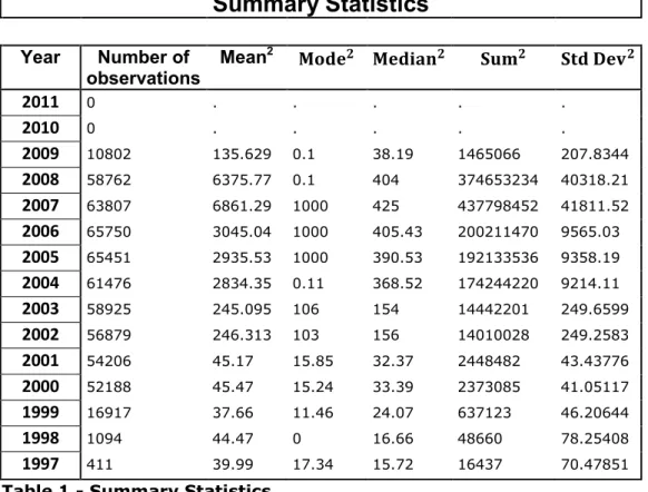
The total sales by year and country for the retained firms constitute on average 0.001%, a breakdown by country is given in Annex 2 along with some general descriptive statistics. Nonetheless there are years, notably the 2005 to 2008 windows where the total sample of firms sometimes constitutes upwards of 5% of the aggregate GDP. Therefore we have a sample that’s at best a snapshot of minute portion of the economy. Even so the sample is large in number of firm observations and seemingly random in its selection of them which is good for analysis. Thus, I will need to control for a variety of possible sample-selection and composition bias possibilities.
Summary Statistics
Year
Number of
observations
Mean
22011
0 . . . . .2010
0 . . . . .2009
10802 135.629 0.1 38.19 1465066 207.83442008
58762 6375.77 0.1 404 374653234 40318.212007
63807 6861.29 1000 425 437798452 41811.522006
65750 3045.04 1000 405.43 200211470 9565.032005
65451 2935.53 1000 390.53 192133536 9358.192004
61476 2834.35 0.11 368.52 174244220 9214.112003
58925 245.095 106 154 14442201 249.65992002
56879 246.313 103 156 14010028 249.25832001
54206 45.17 15.85 32.37 2448482 43.437762000
52188 45.47 15.24 33.39 2373085 41.051171999
16917 37.66 11.46 24.07 637123 46.206441998
1094 44.47 0 16.66 48660 78.254081997
411 39.99 17.34 15.72 16437 70.47851Table 1 - Summary Statistics
4
Firm-Level Volatility
Consider the time series of a random variable Xt. the volatility of Xt is defined as the time series of standard
deviations of 3-year windows of Xt. Formally we compute the time series for volatility of Xt as
√∑ Where is the average between t-1 and t+1.
For every firm a time series where is represents the growth-rate of real sales for the company, the deflator being the PPI – the aggregate producer price index for the European Economic Area. These standard deviations are then averaged across all the firms in a year to arrive at the average volatility for every year. Therefore we remove the average growth rate for a given firm in a given 3-year window and thusly control for firm-specific aspects that affect the growth rate of sales. If on the
contrary, we would have computed the standard deviation across all the firms, then this cross section would have been (more) vulnerable to a compositional bias through the medium of fixed firm-effects.
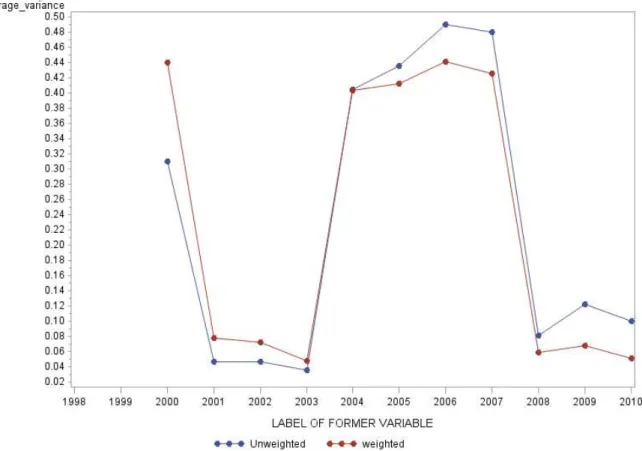
Figure 1- Firm-level volatility for the whole sample
As illustrated in Figure 1, volatility at firm-level exhibits a persistent ‘leveling’ trend after the boom years of the noughties and its correction in 2007. The graph plots volatility per year as a decimal of
percentages. In order to build a more representative measure, firm-level volatility measures are weighted by the firm’s share of turnover of a given year in its country’s total turnover in the sample of that same year. This weighted measure is also graphed in Figure 1. Although both weighted and unweighted measures display the ‘leveling’ tendency, it’s source may be called into question. That’s because it could very well be a feature specific to the sample or the variable in use. Although in this exercise a different proxy for performance could not be used, I need to respond to these eventualities.
4.1 Bias due to Price Divergence
The levelling of volatility at firm level may be due to differences in the prices at firm level. However, price deflators at sector-level don’t exist, therefore I cannot analyse the volatility of growth rates of real sales, and must be content with nominal values. To examine the eventuality of firm-level price
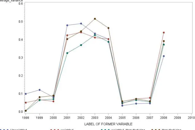
divergence, a subset of our sample is examined. I separated all manufacturing firms to see if there was a price divergence at the 2-digit NACE code level. Then four-digit deflators are used to adjust net-sales to real measures. Figure 2 presents the average weighted and unweighted measures of volatility of the sub-sample of manufacturing firms and compares this to the whole sample on the same graph.
Figure 2 - Comparison of Manufacturing Subsample with Total Sample - Detail
and whole graph
The figure suggests that the evolution of average volatility is similar to the growth rate of nominal sales for the firms in the full sample and for firms in the manufacturing subsample. Furthermore the figure shows that the growth rate of nominal and weighted real sales is the same. This result suggests that the levelling trend in volatility is not driven by firm-level price divergence. Nonetheless it may be the case that price-divergence operates at the four-digit level. Further studies could rule out that possibility by using the number of employees as a real measure of growth rate.
4.2 Bias due to Sample Composition
The sample is taken from the AMADEUS database for all years from 1997-2011, but the sample
increases drastically between the years 2001-2007. This is because certain reporting laws can into effect or were changed on a country-basis which means that there is an increase in available data notably in Austria. As a consequence this raises the possibility that the observed trend is due to a compositional bias. Firms that are incorporated into the dataset from that period may potentially be more exposed to the financial crisis’ exogenous shock either because their sectors are more vulnerable or due to firm-specific attributes such as age, size, management competence, independence, debt-levels, or provenance. One remedy to this problem is simply to track the evolution of the firms initially in the sample’s volatilities, but this would induce a survivorship bias which doesn’t remedy the source of the
concern. Therefore in order to show that the trend is not due to a compositional bias, four exercises are undertaken.
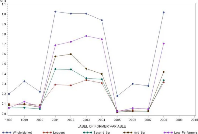
First, the sample of firms is divided up every year into five quintiles according to the level of sales. A firm enters a given quintile if it remained in the quintile for two consecutive years. The top quintile, for example is defined as follows:
( )
Where and are consecutive windows.
Next I examined whether the observed trend in volatility is driven by any specific quintile by seeing whether or not the levelling effect is a product of averaging with quintiles driving volatilities in opposite directions, or whether it’s a pervasive phenomenon across quintiles. Figure3 clearly shows that the levelling of volatility is not driven by any specific quintile but rather that it’s pervasive across the sample and not restricted to any section of the distribution. Nonetheless, this finding does not fully account for the possibility that firms in the sample and in each quintile are composed by firms more exposed or susceptible to shocks after 2002: all the quintiles may be composed of firms that were intrinsically more vulnerable to 2006’s exogenous shock.
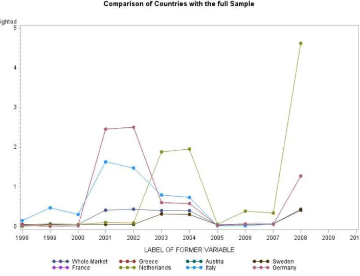
It could also be that it’s in fact firms from a given country instead of firms of a given size that are driving the trends in volatility across the sample. That’s why I checked each country against the others to see if any given country leads the sample or flattened an otherwise pervasive upward trend. I find that there is an averaging effect in the years 2001 to 2005 whereby the Dutch sample lowers the aggregate variance whilst the Italian and German samples increase in volatility. Then it’s the turn of the Dutch section to be victim of an averaging effect. Nevertheless we see all the countries eventually converge. This means that it’s likely that some measure of bias due to sample composition is present but that the sample ‘responds’ well to it once the initial ‘shock’ of a sharp increase in observations has passed and large numbers of observations become pervasive across countries of origin.
Figure 4 - Comparison of Countries to the full sample.
4.3 Firm-specific uncertainty
As a second exercise to control for the eventuality that firms that enter the sample in 2002 are more vulnerable to the financial crisis, I looked for the component of volatility that is not explained by level characteristics that are changing in the sample. Therefore I ran a pooled regression of the firm-level standard deviations ( ) on a vector of firm characteristics ( ) that contains the log of the share of firm sales in the total of the sample retained by country and the log of the firm’s age:
The residual ( ) is then aggregated to produce a time-series of the unpredictable component of firm-level volatility. This exercise was repeated for weighted measures of variance. Unfortunately a suitable proxy for firms’ activity levels was not present in the dataset and this could not be included as a component of the vector .
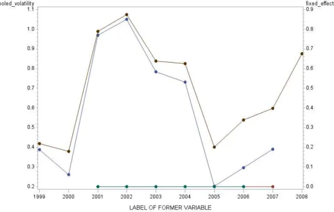
Nonetheless the observed time series, although able to refute that the observed trend is the product of compositional bias, begs the question of whether or not there may be other firm-specific variables that account for the levelling trend. Indeed there may be omitted firm-specific variables that lead to a compositional bias. To rule out this possibility, I ran fixed-effect regressions3 with firm-dummies to
remove the observable and unobservable effects of firm-specific variables on volatility. Removing these effects thus leave only the orthogonal component of unpredictability to fixed firm characteristics.
Formally, I ran the following regression where is the set of firm dummies and is the set of controls, namely the log of age and the firm’s share of sales for the sample:
3 Of a random sample of 30000 firms 10 times (a naïf Monte Carlo experiment) and used their averages
Figure 4 plots and compares the time series of the unpredictable components volatility of the weighted and unweighted pooled and fixed-effect regressions. The figure plots the unweighted pooled effect on the left axis and the rest of the regressions on the right axis. As we can see the ‘level’ trend is evidenced by the collapse of the curve and we can rule out that the uncertainty is simply the result of including more firms in the sample in 2002. If the observed trend was simple the result induced by the fact that the firms chosen in 2002 were simply less volatile, removing firm-specific components of all firms in the sample eliminates the component that is less volatile for new firms. Therefore if the observed trend still persists, we can rule out that a compositional bias is the driver of the trend.
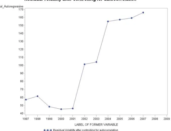
Figure 6 - Residual volatility after controlling for autoregressive effects
5
Firm Level Volatility by Sector
After I verified the robustness of the ‘level’ trend discovered in the volatility of the sample, I analysed the volatility by sector. That’s because any given sector might be at the root of the observed trend. Thus, to verify that this is not the case I ran the following regressions for each two digit sector:
; ;
where D is a set of sector specific time dummies. I ran both these regressions on weighted and unweighted measures of growth for all sectors. By running all these regressions I can construct a time-series for the weighted and unweighted average firm-level volatility after controlling for age and size and a firm-specific intercept. For each two digit sector, Table 2 reports the average estimated coefficient on for each year from the pooled regression without firm-level fixed effects. Table 2 shows that the all changes in variance were reflected in each sector, with a notable exception being the computer and optical in the wake of the internet bubble and their associated industries namely, fabricated metals like rare earth products and non-metalic minerals like quartz, which have coefficients about twice the gradient of other sectors. These are joined only one year later by petroleum, together they drive a short-lived uptick in volatility at the firm-level between 2001 and 2002. Looking at the evolution of the petroleum sector over the full time period leads me to hypothesise that shocks to both demand and supply will be compensated in the short run by governments.
UN-WEIGHTED
WEIGHTED
SECTOR
1999
2000
2001
2002
2003
2004
2005
2006
2007
2008
1999
2000
2001
2002
2003
2004
2005
2006
Water Collection and
Supply 0.0097 0.00778 -0.0033 -0.0027 -0.0079 0.0097 0.00778 -0.0033 0.0004
Electricity, gas, air,
steam 0.008 0.0069 -0.0023 -0.0016 -0.00059 -0.0058 0.008 0.0069 -0.0023 0.0006 -0.0006
Repair and Installation of Machinery and Equiptment -0.002 0.0052 0.0053 -0.0035 -0.0023 -0.0004 -0.0012 -0.0057 -0.002 0.0051 0.00538 -0.00345 -0.0023 -0.0004 Other Manufacturing 0.0114 0.0114 -0.002 -0.002 -0.0037 0.0114 0.01138 -0.00197 -0.002 Manufacture of furniture 0.0118 0.0111 -0.0024 -0.0019 -0.00017 -0.002 0.0117 0.011 -0.00239 -0.0019 -0.0002 Transport equiptment 0.003 0.003 -0.0063 -0.0053 -0.00072 0.0031 0.003 -0.00633 -0.0053 -0.0007 motor vehicles 0.0072 0.0065 -0.0031 -0.0024 0.0001 -0.00008 -0.0055 0.0072 0.0065 -0.00313 -0.0024 0.0001 -0.0001 Machinery 0.0097 0.0098 -0.0024 -0.0018 0.0001 -0.00006 -0.0042 0.0097 0.0098 -0.00236 -0.0018 0.0001 -0.0001 Electrical Equiptment 0.0111 0.0113 -0.0028 -0.0026 0.0001 -0.0004 -0.0004 -0.0057 0.0111 0.0113 -0.0028 -0.0026 -0.0004
Computer and Optical -0.0005 0.0212 0.0212 -0.0012 -0.0009 0.0001 -0.0043 -0.00051 0.0212 0.0212 -0.0012 -0.0009 0.0001
Fabricated Metals -0.0006 0.0181 0.0173 -0.0013 -0.001 0.00004 0.0001 -0.0039 -0.00064 0.0181 0.0173 -0.00134 -0.001 0.00004
Basic Metals -0.0003 0.0126 0.0118 -0.0022 -0.0018 0.0002 -0.0033 -0.00032 0.0126 0.0117 -0.00215 -0.0018 0.00017
Non metalic Minerals 0.0254 0.0263 0.0023 0.0022 0.0254 0.0263
Rubber and Rubber
Products -0.0003 0.0095 0.0092 -0.0018 -0.0014 0.0002 -0.0019 -0.00034 0.0095 0.0092 -0.00183 -0.0014 0.00017
Basic Pharmaceuticals 0.0152 0.0154 -0.0014 0.0001 -0.004 0.0152 0.0154 -0.00144 0.00014
Chemical and
Chemical Products 0.007 0.0064 -0.0017 -0.0011 0.0001 -0.0052 0.007 0.0064 -0.00169 -0.001 0.00011
6
Aggregate Volatility
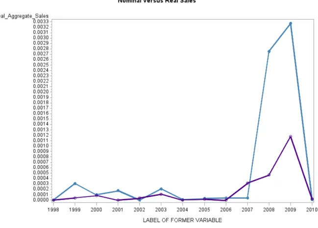
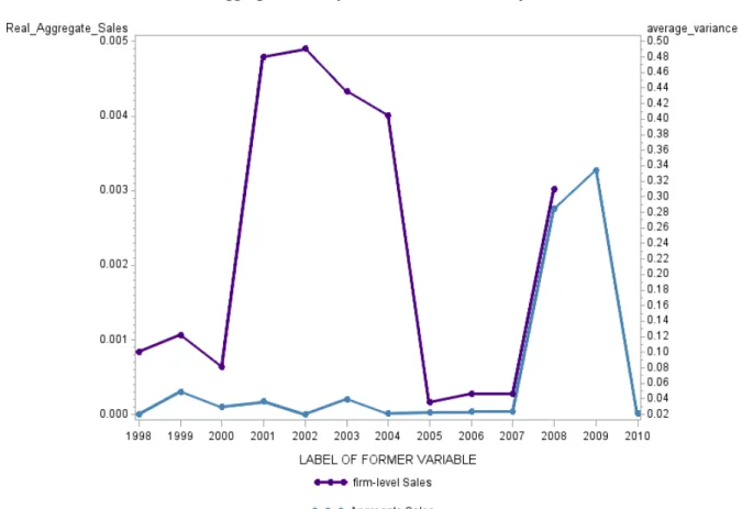
I’ve discovered that the evolution of aggregate volatility converges towards that of the firms’ in my sample after the financial crisis whereas during the boom years firm-level volatility increases markedly and diverges. Many authors have remarked that aggregate growth has become more stable in recent years, and some have suggested that there is an association between the aggregate level volatility and non-listed firms’ volatility. Figure 5 plots the time series for growth rates of both nominal and real aggregate final sales of the European Union 17. The volatility of aggregate sales displays a large
increase starting from 2007 to 2009 coinciding with rises in firm-level volatility in 2005 and 2007. As we can see from the fact that nominal and real GDP growths are similar until 2007, inflation is not a concern for my purposes. Inflation becomes an issue in the 2007 to 2010 windows, the duration of the first dip of the financial crisis characterised notably by a massive quantitative easing among other non-conventional responses. When this time series is compared to that of the firm-level volatility we see that
convergence and levelling trends are evident.
Figure 8 - Volatility of Growth Rate of aggregate final sales and firm-level sales
7
Variance Decomposition
To understand the mechanics of convergence in my sample, I’ve decomposed the variance of the aggregate growth rate of turnover in the Amadeus Database into a variance and covariance component. Firstly I verified that my sample displayed similar characteristics at the aggregate level to those of GDP for the European Union. Contrary to aggregate total sales, my sample exhibits a recovery of sorts in 2008. This is due to the fact that although aggregate total sales was still steeped in recession there was a moderate recovery as part of the European Union’s double dip recession that evidently mostly affected firms the size of our sample. Another reason is the fact that our sample’s size varies. Both of these facts together mean that there is a certain level of noise to the growth rate of the AMADEUS database’s aggregate sales. This influence may tend to induce an upward bias in the trend of volatility of the growth rate of total sales in my sample precisely at those periods with more observations. This problem is particularly evident in the year 2001 of my sample where a sharp increase in the number of observations induces a notably sharp rise in the volatility of growth. Another way to observe this problem would be to look at lower levels of aggregation, for example two-digit NACE sector levels. To conduct variance decomposition, the following notation is introduced. Let be the growth rate of aggregate real sales deflated by the aggregate PPI for the EU17, be the growth rate of real sales for firm i , and be the share of sales for firm i in the total sales of its country from the AMADEUS sample, all in year t. Let be the growth rate of real sales for each sector m deflated by sector-specific deflators. Let be the growth rate of rate of real sales for each country k deflated by the aggregate PPI for the EU17. Also, let denote the variance of for any generic variable Z, and be the covariance between and .
Note that ∑ . Then, using the definition of variance, and assuming that for all the firms i and all the years t, the variance of aggregate growth in year-on-year, , can be decomposed into two terms: the first is related to the firm-level variance of turnover (simply the variance) and the second reflects the covariances between the growth rates of sales at different firms (covariance component):
∑ ∑ ∑ ∑ ∑ ∑ ∑ ∑ ∑ ( ) ∑ ∑ ∑ ∑ ∑ ∑
The first part of that equation is the variance component and the second part represents the covariance component. Figure 7 shows the evolution of each of these terms and compares them to total variance.
7.1 Conclusions
The European economy is experiencing a convergence of aggregate- and firm-level volatility of small and medium businesses. This study demonstrates interesting differences between the 1999 crisis, driven by the internet-bubble and the 2007 crisis driven by the financial sector’s (partial) collapse. Whereas during the internet bubble in year 1999 we can see that variance is driven by the sectoral covariance
component versus the country covariance component, in the wake of the financial crisis, we see that the aggregate variance of the Eurozone was driven by the country covariance component. What’s more the 2006 financial crisis was preceded by an increase in inter-firm covariance, forewarning of the
momentous corrections to come. This fundamental difference between these two events has hopefully informed government policy in its wake.
In fact consensus macro-economic policy would explains this quite well. Whereas the first’s response focussed on easing the process of correction, the second should and did (in the beginning) focus on fundamental arbitrage between the private and public sector spending and compensate the reduced private spending. Thus from this perspective, the current focus on austerity doesn’t seem as judicious as it’s trumpeted.
Davis and Kahn’s study’s conclusions are in line with the findings in this article. If firms’ revenue is further into the future due to increasing investment in durable inventory (Davis & Kahn, 2008), it makes sense that they are more sensitive to expectations about the future proxied by interest rates and income.
Whereas Comin and Mulani find that McConnell and Perez-Quiroz’s conclusions do not fit with their findings, from this study, their explanation of the decrease in volatility of firm and aggregate levels are consistent with this study’s findings. They argue that new inventory management methods such as just-in-time inventory management (which leads to a decline in stocks and losses due to stock levels) are the source of a decline of volatility at the firm-level.
Research of macro-determinants of volatility argue that part of the decline in aggregate volatility is due to more effective monetary policy that helps stabilise shocks to the economy at the aggregate level. Although an increase in the efficacy of monetary policy may account for only 30% of the observed reduction in aggregate volatility, we can see that these mechanisms have had an effect at the firm level when decomposed. Indeed looking at the 2008 and 2009 windows in our study we find that when momentous monetary easing tactics have been implemented in the beginning of the crisis in Europe, they did lead to a decrease in the average variance and an increase in the variance is observed once a more stringent focus on austerity measures was implemented. This explanation is therefore relevant to this study.
Comin and Mulani’s argue that it’s a focus on embodied versus disembodied innovations that may explain their observed symmetric trends in volatility at the firm- and aggregate-levels. That’s because firms have less incentive to invest in fundamental research than product research, and that means that their marketed widgets will demonstrate the commonly observed volatile market reactions: new products are more volatile than disruptive innovations. This argument is inconsistent firstly because not all disruptive technology gains a foothold (not all great ideas make it to and in the market) and secondly because we would expect product-focussed spinoffs and product-associated firms to demonstrate the increased volatility they observed. Presumably these types of companies would fall in the AMADEUS sample, and our study displays the opposite trend.
Aghion et.al. argue that credit constraints proxied by financial development (Aghion, Angeletos, AbhijitBanerjee, & Manova, 2010) play a central role in firm-level and aggregate level volatility. The complementary theory of Easterly et.al. would add that it’s a given country’s institutional endowment that induces this effect (Easterly, Islam, & Stiglitz, 2000). Although these authors would recognise that the effect is less pronounced in developed countries like those found in the Amadeus sample, I find that countries with very different levels of financial development like Ireland and Greece have broadly similar volatility levels over the time period analysed.
Conversely, it may in fact be the case that what we’re observing in my antagonistic conclusions is the divergent character of two very different industrial organisations. Whereas industrial policy or business regulation in America is geared towards promoting entrepreneurship and the growth of companies, in Europe there are severe impediments to the growth of medium size firms into large ones. These impediments include social charges on salaries, restrictive employment contracts, and the loss of tax breaks once the Small and Medium size Enterprise threshold is crossed.
8
Works Cited
Aghion, P., Angeletos, G.-M., AbhijitBanerjee, & Manova, K. (2010). Volatility and growth: Credit constraints and the composition of investment. Journal of Monetary Economics, 57, 246-265. Aghion, P., Bacchetta, P., Ranciere, R., & Rogoff, K. (2006, March). Exchange rate volatility and
productivity growth : the role of Financial Development. NBER, 1-48.
Blanchard, O., & Simon, J. (2001). The Long and Large Decline in U.S. Output Volatility. Brookings
Papers on Economic Activity, 2001(1), 135-164.
Campbell, J. Y., Lettau, M., Malkiel, B. G., & Xu, Y. ( 2001, February). Have Individual Stocks Become More Volatile? An Empirical Exploration of. The Journal of Finance, 56(1), 1-43.
Comin, D., & Mulani, S. (2006, May). Diverging Trends in Aggregate and Firm Volatility. The Review of
Economics and Statistics, 88(2), 374-383.
Davis, S. J., & Kahn, J. A. (2008, Fall). Interpreting the Great Moderation: Changes in the Volatility of Economic Activity at the Macro and Micro Levels. Journal of Economic Perspectives, 22(4), 155-180.
Davis, S., Haltiwagner, J., Jarmin, R., & Miranda, J. (2006, May). Volatility and Dispersion in Business Growth Rates: Publicly Traded versus Privately Held Firms. NBER Macroeconomics Annual 2006,
21.
Easterly, W., Islam, R., & Stiglitz, J. E. (2000). Shaken and Stirred: Explaining Growth Volatility. Annual
World Bank Conference of Development Economics, 191-213.
Gabaix, X. (2011). Power Laws and the Granular Origins of Aggregate Fluctuations. Econometrica, 79(3), 733-772.
McConnell, M. M., & Perez-Quiros, G. (2000, December). Output Fluctuations in the United States: What Has Changed Since the Early 1980’s? American Economic Review, 90(5), 1464-1476.
Phillipon, T. (July 2003). An Explanation for the Joint Evolution of Firm and Aggregate Volatility. Stern School of Business, Department of Finance. New York: New York University .
Stock, J. H., & Watson, M. W. (2003). Has the business cycle changed and why? NBER Macroeconomics Annual 2002. MIT Press.
Wang, P., & Wen, Y. (2009, May). Financial Development and Economic Volatility: A Unified Explanation.
9
ANNEX : Variance Decomposition
This annex is dedicated to the decomposition of aggregate variance into the variance of sectorial growth, the variance of growth between counties, and inter-firm covrariance. The growthrate of the aggregate variable of interest ( is related to interfirm, sectoral and country growths as follows , ) by :
∑ ∑ ∑
Where are the relevant weights. Aggregate variance of between and can be expressed as: ∑ ∑ ∑ ∑ ∑ ∑ ∑ ∑
Imposing the restriction that sectoral and country weights are constant during the interval ∑ ∑ ∑ ( ∑ )
Expanding and manipulating we obtain the variance-co-variance decomposition:
∑ ∑ ∑ ∑ ∑ ∑ ∑ ( ∑ ) ( ∑ ) ( ∑ ) ( ∑ ) ( ∑ ) ( ∑ ) ∑ ∑ ∑ ∑ ∑ ∑ ∑ ( ∑ ) ( ∑ ) ( ∑ ) ( ∑ ) ( ∑ ) ( ∑ ) ∑ ( ) ∑ ∑ ∑ ∑ ∑ ∑