Fortin: Département d’économique, Université Laval and CIRPÉE, CIRANO and IZA [email protected]
Jacquemet : Paris School of Economics and University Paris I Panthéon-Sorbonne [email protected]
Shearer: Département d’économique, Université Laval, CIRPÉE, CIRANO and IZA [email protected]
Cahier de recherche/Working Paper 10-34
Labour Supply, Work Effort and Contract Choice: Theory and
Evidence on Physicians
Bernard Fortin
Nicolas Jacquemet
Bruce Shearer
Abstract:
We develop and estimate a generalized labour supply model that incorporates work
effort into the standard consumption-leisure trade-off. We allow workers a choice
between two contracts: a piece rate contract, wherein he is paid per unit of service
provided, and a mixed contract, wherein he receives an hourly wage and a reduced
piece rate. This setting gives rise to a non-convex budget set and an efficient budget
constraint (the upper envelope of contract-specific budget sets). We apply our model to
data collected on specialist physicians working in the Province of Quebec (Canada). Our
data set contains information on each physician’s labour supply and their work effort
(clinical services provided per hour worked). It also covers a period of policy reform
under which physicians could choose between two compensation systems: the
traditional fee-for-service, under which physicians receive a fee for each service
provided, and mixed remuneration, under which physicians receive a per diem as well
as a reduced fee-for-service. We estimate the model using a discrete choice approach.
We use our estimates to simulate elasticities and the effects of ex ante reforms on
physician contracts. Our results show that physician services and effort are much more
sensitive to contractual changes than is their time spent at work. Our results also
suggest that a mandatory reform, forcing all physicians to adopt the mixed remuneration
system, would have had substantially larger effects on physician behaviour than those
observed under the voluntary reform.
Keywords: Labour supply, effort, contracts, practice patterns of physicians, discrete
choice econometric models, mixed logit.
1
Introduction
Empirical labour-supply models have played an important role in economic policy analysis. Sim-ulations from these models have been used to measure and predict the effects of tax, welfare and social policies on labour-force participation and hours worked in the economy. Examples include Heckman (1974); Hausman (1980); Hoynes (1996); Blundell, Duncan, and Meghir (1998); see Blun-dell and MaCurdy (1999) for a survey. The parallel, but related, empirical contracting literature has focussed on the effect of monetary incentives on effort and productivity (Paarsch and Shearer, 2000; Shearer, 2004), paying attention to the endogenous choice of a compensation system on the part of agents (Lazear, 2000) and heterogeneous responses to incentives (Chiappori and Salani´e, 2003). Generalized models, which incorporate effort decisions into traditional labour-supply models, al-low for a richer policy evaluation environment, particularly in settings where productivity is not proportional to time spent at work. Such models can be used to measure and predict the effects of wages and contracts on hours worked and productivity, capturing responses that may be missed in traditional models; they also permit cost and welfare comparisons across contracts.2 Yet, to date, little attempt has been made to combine contracting models with labour-supply models in empir-ical work.3 This paper addresses this issue. We develop and estimate a generalized labour-supply model using a unique data set on physicians’ practice behaviour.
Physician behaviour is well-suited to analysis within a generalized model. Physicians can affect both their time spent at work and the volume of services that they provide while at work through effort (McGuire, 2000). Recent estimates of time-based labour supply elasticities have been provided by Showalter and Thurston (1997) and Baltagi, Bratberg, and Holm˚as (2005).4 Estimates of the effects of compensation policies on physician behaviour have been provided by Gruber and Owings (1996) and Devlin and Sarma (2008). Our approach allows us to measure these effects within the context of a parsimonious economic model and to measure the effects of contracts on the time spent
1The authors thank the Coll`ege des m´edecins du Qu´ebec for making its survey data available and the R´egie
d’assurance-maladie du Qu´ebec and Marc-Andr´e Fournier for the construction of the database. This article was partly written while Fortin and Shearer were visiting the University Paris 1 Panth´eon-Sorbonne. We thank participants at the Maurice Marc-hand Meeting in Health Economics (Lyon), the CIRP ´EE Workshop on Applied Micro-Econometrics (Qu´ebec), the ADRES workshop on the Econometric Evaluation of Public Policies (Paris), the Canadian Economics Association (Montr´eal), the European Workshop on Econometrics and Health Economics (Thessalonique), the European Economic Association (Vi-enna) and the Econometric Society Winter Meeting (Chicago). We also thank seminar participants at CREST, the Free University of Amsterdam and Paris-Dauphine University. We are grateful to Michel Truchon as well as Bruno Cr´epon, Arnaud Dellis, Brigitte Dormont, Pierre-Yves Geoffard, Guy Laroque, Pierre-Thomas L´eger and Marie-Claire Villeval for useful discussions and comments. We acknowledge research support from the Canadian Institute of Health Research (CIHR) and the Canada Research Chair in Social Policies and Human Resources at the Universit´e Laval.
2Ferrall and Shearer (1999); Margiotta and Miller (2000); Paarsch and Shearer (2009); Copeland and Monnet (2009)
are among those who have implemented empirical contracting models to investigate the welfare properties of different contracts and the cost of moral hazard within the firm.
3One important exception is Dickinson (1999) who analyses a model incorporating on- and off-the-job leisure, that is
tested using controlled laboratory experiments.
4The effect of incentives on physicians’ choice of location has also been analysed within the context of the labour
per service, a suggested measure of health-care quality (Ma and McGuire, 1997).5 It also allows us to generalize treatment-effect estimates to predict the effects of compensation policies ex-ante6and, in some cases, to make welfare comparisons across contracts.
We develop a simple model which we use to motivate and develop our general approach. We specify utility as a function of consumption, hours of work and effort (measured by the volume of services produced per hour of work). Contracts are composed of an hourly wage rate and a piece rate per unit of service provided. The marginal return on an hour of work is thus endogenous and depends on effort. Similarly, the marginal return on effort depends on hours of work. These nonlin-ear prices are similar to those obtained in quantity/quality models (Becker and Lewis, 1973). Some comparative static results are derived; we show that the compensated (hicksian) supply curves of hours and services are positively sloped in the wage rate and the piece rate, respectively. In a more realistic model, the worker has the choice between two contracts: one composed uniquely of a piece rate and another composed of a wage rate per hour worked and a reduced piece rate. We show that this environment gives rise to a non-convex budget set, from which we derive an efficient budget constraint (the upper envelope of the contract-specific budget constraints).
We apply our model to the practice behaviour of specialist physicians working in the Province of Quebec (Canada) between the years 1996-2002. All these physicians work within the Quebec public Health-Care System. Our data contain information on individual physician labour supply (weekly hours spent seeing patients, weekly hours spent performing administrative tasks or teach-ing, and weeks worked per year) as well as the number of services provided by each physician per year. The observation period also spans an important reform in physician compensation which we exploit to identify our model. Prior to 1999, most specialist physicians in Quebec (92%) were paid fee-for-service (FFS) public contracts, receiving a fee for each service provided. In 1999, the gov-ernment introduced a mixed remuneration (MR) scheme, under which physicians received a per diem, paid per hour worked, and a reduced fee-for-service. A notable aspect of the reform was its voluntary nature; from the time the mixed compensation system was introduced, two sub-samples of physicians are observed: those who adopt the MR system and those who remain under the FFS system. We exploit this change in the compensation system to identify the physicians’ preference parameters.
To estimate the model, we assume that preferences are (directly) independent of the compensa-tion system. This implies that racompensa-tional, unconstrained physicians will locate on the efficient budget constraint – the budget constraint that maximizes a physician’s income for each possible combi-nation of practice variables in his choice set. We derive the efficient budget constraint from our knowledge of the physician’s contracts. We pay careful attention to the complications created by
5Recent empirical work suggests that compensation policies do influence physician behaviour in these directions
(Dumont, Fortin, Jacquemet, and Shearer, 2008).
6See Marschak (1953); Heckman and Vytlacil (2001), and Todd and Wolpin (2008) for a discussion of ex-ante policy
the institutional constraints imposed on these contracts within the Quebec Health-Care System (e.g., income ceilings, regionally differentiated remuneration, constraints on the choice of the compensa-tion system at the individual level). The simultaneous modelling of the allocacompensa-tion of time, work intensity and institutional constraints introduces strong nonlinearities into the budget constraint. To account for these nonlinearities in estimation, we discretize the choice set available to physi-cians (Zabalza, Pissarides, and Barton, 1980). This methodology is relatively free of restrictions (MaCurdy, Green, and Paarsch, 1990), imposing only that the marginal utility of income is positive (van Soest, 1995).
We then solve for the utility-function parameters that generate the observed practice patterns as optimal choices along the efficient budget constraint. To account for selection we allow for het-erogeneity in preferences (both observable and unobservable), estimating a mixed-logit model (Mc-Fadden and Train, 2000). To minimize the effects of functional forms on our results, we use a flexible (quadratic) utility function, which can be viewed as a second-order approximation to the true utility function. In order to limit computational time in estimation and to reduce the problem of hetero-geneity in the nature of services provided, we restricted our sample to one speciality –pediatrics. This specialty provides high variability in the participation in MR – 44% of pediatricians opted for MR in the year 2000 as compared with 31% for all specialities. The voluntary nature of the reform further complicates estimation, for the following reason. The decision to adopt MR was not indi-vidual specific, but determined at the department level within hospitals.7 Consequently, individual physicians could be constrained in their choice of a compensation system. Accounting for con-straints on choice leads to a mixture of likelihoods wherein the probability of being constrained is estimated along with the other parameters.
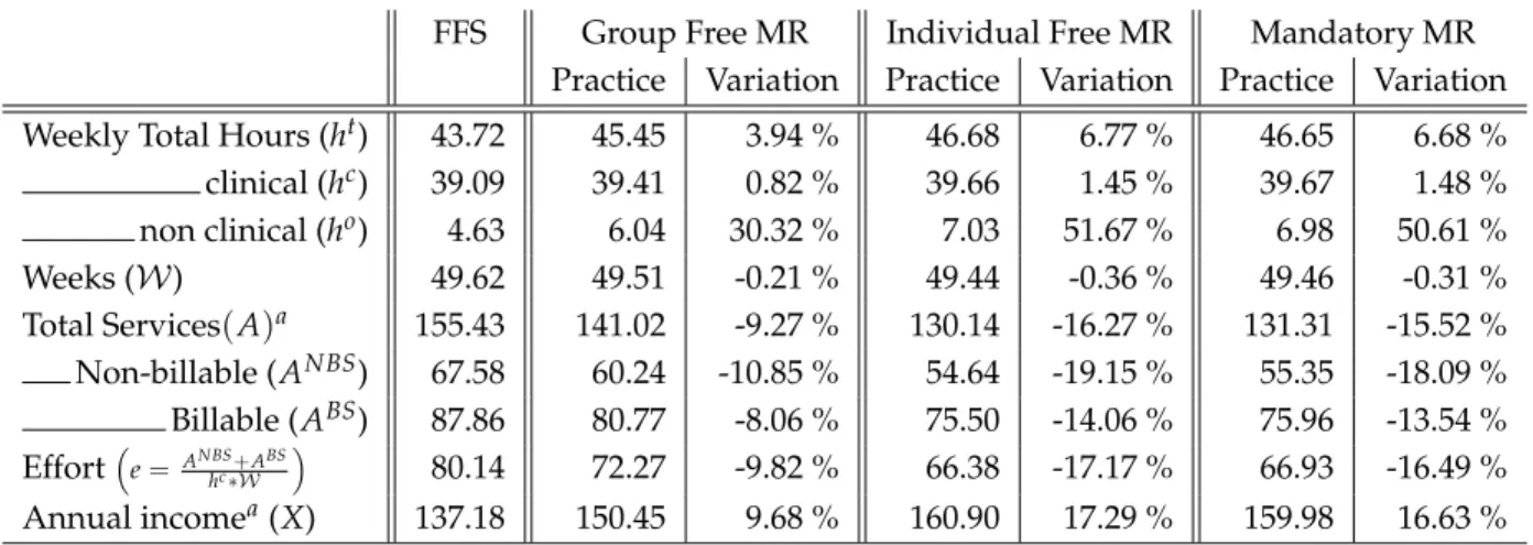
Elasticities and the effects of policy reforms are simulated through changing appropriate pa-rameters of the budget constraint and allowing physicians to re-optimize. Our results suggest that labour supply (weekly hours and weeks) elasticities are quite small while the (compensated) elas-ticities of effort and services with respect to the fee per service are much stronger, being estimated at about 0.3 and 0.4 respectively. Non-clinical hours (spent on administrative and teaching activities), that are not remunerated under a FFS contract, are quite sensitive to compensated changes in the fee per service, with an elasticity of -0.4. Our results also suggest that the changes in incentives brought about by the 1999 reform strongly affected physician behaviour. Services completed decreased by 9% and non-clinical hours increased by 30%. What is more, work effort decreased, suggesting that the quality of care may have increased (more time spent per service). A mandatory reform, forcing all physicians to work under MR, would have reduced services by 15% and increased non-clinical hours by 50%. However, these larger effects are not due to unobserved heterogeneity and selection, but rather to the constraints placed on individual choice in the observed reform.
7Members of each department (groups of specialists working in the same field) would vote on the adoption of MR;
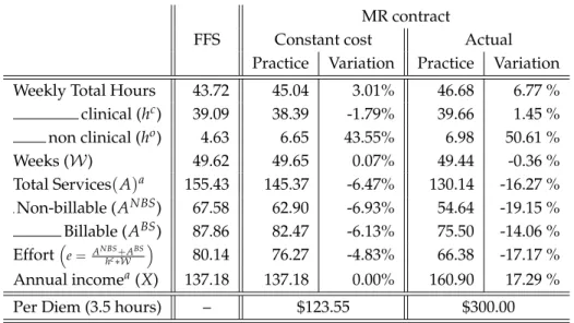
The reform was also costly. Payments to physicians increase by over 9%. This is due to the large per diem that physicians were paid for working under MR. We investigate the welfare effects of constant-cost contracts under voluntary participation in MR. Under such circumstances services provided would decrease relative to the fee-for-service contract by 6.47%. Yet the welfare impli-cations are inconclusive: clinical hours worked would decrease by only 1.72% and time spent per service would increase by 4.83%.
The rest of the paper is organized as follows. Section 2 develops the basic model that we will use in this paper. Section 3 describes the institutional details of the fee-for-service and mixed re-muneration systems and derives the physician’s budget constraint. Section 4 presents our data and summary statistics. Section 5 adapts the model of Section 2 to the institutional details of the Qu´ebec reform and develops our empirical model. Section 6 describe our empirical results and the policy simulations. Section 7 presents our conclusions.
2
A generalized model of labour supply
We present a static model of labour supply behaviour under linear contracts. Our model allows for decisions over hours of work and effort. Our goal is to motivate our empirical analysis and our estimation strategy within a simplified setting. Later we will adapt the model to fit the specific institutional details of physician labour supply in Quebec.
Preferences are represented by the strictly quasi-concave and twice-differentiable utility func-tion
U(X, h, e), (1)
where X is consumption, h is hours of work, and e is effort. We assume
UX >0, Uh <0, Ue<0. (2)
Effort is determined by the number of services, A, performed per hour of work; we have8
A=eh. (3)
In some settings, time spent per service can be taken as a measure of quality of services – Ma and McGuire (1997) have suggested such a measure in the case of physicians. This amounts to= 1/e
8One interpretation of (3) is a (Cobb-Douglas) production function. In a more general model this function could be
written as A=A(e, h; z), with e denoting a measure of effort such as the ratio of effective hours of work to hours at work and ¯z denoting an exogenous vector of inputs that affect the marginal productivity of effort and hours worked. This could be decomposed into two sub-matrices: z1containing physical capital (e.g., hospital equipment) and z2containing human capital, or personal, characteristics ((e.g., age, experience). Such a specification would also allow for more complex substitution patterns between effort and hours (perhaps due to fatigue).
in our model, changes in which are a valid measure of changes in time spent providing services if on-the-job leisure is fixed.9
The budget constraint is given by
X =wh+pA+y, (4)
where X is consumption (the price of which being normalized to one), w is the wage rate, p is the fee per unit of service and y is non-labour income. Variation in w and p are treated as exogenous.10 Note that the budget constraint, (4), is general enough to account for many contracts of interest: setting w = 0 and p > 0 gives the FFS contract, setting w > 0 and p > 0 gives a mixed contract, while setting (w>0 and p =0) gives a fixed-wage contract.
We assume complete and symmetric information. This is a direct consequence of the fact that effort is the ratio of two observable variables: hours worked and services completed.11 What is more, we assume that the worker has complete control over his practice variables – freely choosing both his hours of work and his clinical services.12
In its most general form, our model combines traditional labour supply analysis with a piece-rate model, giving rise to non-linear (and endogenous) prices in the budget constraint. This can be seen by substituting (3) into (4), adding and subtracting peh, and rearranging. This gives X = (w+ pe)h+ (ph)e+yv, where yv = y−phe is the virtual non-labour income. It follows that the marginal return to an hour of work (w+pe) depends on the physician’s choice of effort – the number of services that can be performed in that hour. Similarly, the marginal return to effort (ph) depends on the physician’s hours of work. Since effort changes the number of services performed per hour, the return to effort depends on the number of hours worked. These nonlinear prices are similar to those obtained in quantity/quality models (Becker and Lewis, 1973).
The nonlinear prices give rise to a non-convex budget set (see Appendix A.3). The second-order conditions for optimal behaviour require that the curvature of indifference surfaces be more pro-nounced than the curvature of the budget set. We assume this to be the case and denote the optimal solution(X★, h★, e★). In Appendix A.4 we show that(X★, h★, e★)is equivalent to(X′, h′, A′/h′)which
maximizes the transformed utility:
u(X, h, A) (5)
9This ensures that workers with higher values of 1/e do not simply take longer breaks between services.
10This is consistent with the public health-care system in Quebec. See Feldstein (1970) for an analysis that incorporates
the price-setting behaviour of physicians in a market-based environment.
11Agency problems and moral hazard could be introduced by incorporating random elements into the production
function, perhaps due to differences in the difficulty of tasks or in the marginal utility of on-the-job leisure.
12Within the context of models of physician behaviour this rules out constraints to supply or any demand shocks
that might affect a physician’s practice, allowing us to concentrate on the supply side of the medical market which considerably simplifies the empirical analysis. It seems reasonable within the context of a public health-care system such as in Quebec where long waiting lists for physicians’ services render the demand side of the market relatively passive. Excess demand also reduces any incentive of physicians for demand inducement, which we also ignore.
subject to
X−pA−wh=y,
where (5) is obtained by substituting e = A/h directly into the utility function (1): u(X, h, A) =
U(X, h, A/h). Hence we can identify the parameters determining optimal behaviour using either program: Max (1) s.t. (3) and (4), or Max (5) s.t. (4). In most of the following, we concentrate on the transformed program. One advantage is that all arguments of the transformed utility are well-defined over the whole choice set; effort is not defined in (1) when hours are set to zero.
The non-linearities in the budget constraint complicate the comparative statics of the model. For example, an increase in non-labour income, y, will affect the worker’s choices of effort and hours of work through two channels: the first is the standard income effect, the second is through its impact on the endogenous marginal returns to effort and hours of work. Some results are possible, however. In particular, the fact that the budget constraint is linear in A and h implies that the expenditure function is concave in w and p; hence,
∂ ˜h
∂w ≥0;
∂ ˜A
∂ p ≥0, (6)
where˜indicates that the partial is compensated. Notice however that concavity of the expenditure function does not allow us to sign cross-partial derivatives; hence,
∂ ˜h ∂ p
>
<0. (7)
Similarly, since effort is the ratio of services to hours worked, its compensated partial derivative with respect to p depends on
∂ ˜A
∂ p −
˜ A∂ ˜h
∂ p (8)
which is also unsigned. These results follow from a straight-forward application of duality theory to the problem of maximizing (5) s.t. (4); we include a derivation in Appendix A.5 for completeness.13
2.1 Endogenous Compensation Choice
Introducing the choice of a compensation system complicates the analysis somewhat. We consider two cases: a fee-for-service (FFS), or piece rate, system (X = pA) and a mixed compensation (MR) system (X =wh+α pA), where α<1 denotes the discount rate on the fee-for-service payment (set-ting α = 0 gives a fixed-wage compensation system). To proceed we note that UX > 0. Moreover,
13Similar results are shown in Edlefsen (1981, 1983) using the Hessian matrix from the original maximization problem.
Edlefsen (1981) also shows that a compensated increase in the fee per unit of service will increase both effort and hours of work under a FFS system (p > 0 and w = 0) or a MR system where w is small, if leisure at work (or−e) and leisure outside of work (or−h) are both net substitutes with respect to consumption. Using a somewhat different model, Dickinson (1999) also finds that the effect of a compensated increase in the piece-rate on hours of work is ambiguous.
we assume that preferences are (directly) independent of the compensation system. This implies that rational workers will always select that compensation system that maximizes income for a given(h, A)combination. We therefore proceed in two steps: First we determine the efficient budget constraint, the upper envelope of X attainable from each value of(h, A). Assuming for simplicity zero non-labour income, we have
X(h, A; w, p, α) = max
D∈{0,1}(1−D)pA+D(wh+α pA), (9)
where D is a dummy variable equal to zero when the worker participates in the FSS system and equal to one when he participates in the MR system. Second, the worker solves his (transformed) program by choosing the(X, h, A)combination that maximizes his utility along the efficient budget constraint (9). The choice of a compensation system is then given by
D(h★, A★; w, p, α) =arg max D∈{0,1}
(1−D)pA★+D(wh★+α pA★) (10)
evaluated at the optimal levels of A★, h★.14
This is illustrated in Figure 1 which considers the tradeoff between services and consumption (income), conditional on h★,FFS, optimal hours under the fee-for-service system.15 The budget line FFS has slope p, the marginal monetary return to completing services under FFS; it passes through the origin because hours are not remunerated under FFS. The values of A, X chosen under FFS correspond to the optimal values A★,FFS and X★,FFS. The line MR illustrates the tradeoff between services and income under MR, holding hours fixed at h★,FFS. It cuts the y-axis at wh★,FFSand has slope equal to αp, reflecting the reduced fee-for-service payments received under MR.16
The efficient budget constraint associated with the transformed program is given by the bold line.17 It is piece-wise linear and non convex; this raises well-known problems for optimization and
14The empirical model that we estimate will be adjusted to account for the institutional details of specialist physician
pay in Quebec, including income ceilings and regional payment differentials. This renders the efficient budget constraint more complex, with more segments (which helps identification of the model), yet its derivation follows the same basic steps.
15Notice that optimal hours under FFS are not in general equal to zero, even though w = 0. This is due to the fact
that the marginal return to hours includes both wage and the marginal effect of hours on FFS income (=w+pe). The first-order condition for hours is given by−Uh
UX =w+pe.
16Under a fixed-wage system (α = 0) the monetary return to services provided is zero. A strict interpretation of
the model under these circumstances would imply zero services. However, relatively straightforward extensions to the model would allow for positive services being allowed at the optimum. One possibility is to assume that Ue > 0 for
e< ¯e, due for instance to concern of the physician for his patients. Another, is to assume that monitoring allows for a minimum level of effort to be enforced; see, for example, Lin (2003). We do not elaborate on these possibilities here in order to keep our model simple and since the fixed wage contract is not observed in our empirical data. In any case, our econometric model does not impose Ue<0.
17To be exact, this is the efficient budget constraint conditional on h★,FFS, the unconditional efficient budget constraint
Figure 1: Optimal choices along the efficient budget constraint Services (A) Income (X) FFS RM A_o A_1 B_o
labour supply estimation (Hausman, 1985; MaCurdy, Green, and Paarsch, 1990). Our approach will be to discretize the choice set of workers (physicians), considering only a finite set of values for h, A (van Soest, 1995).
Figure 1 also illustrates potential problems of self-selection. Workers who have a preference for low effort (or high service quality) levels (such as worker A) will tend to choose MR, while those who have a preference for high effort levels (such as worker B) will tend to choose FFS.18A comparison of behaviour across compensation systems will potentially confound the effects of the compensation system with the differences in preferences. The econometric model must therefore allow for both observable and unobservable heterogeneity to take into account of possible selection bias.
18Again, the figure loses some exactness by collapsing a 3-dimensional problem into two dimensions. While an
indi-vidual who chooses Aounder FFS and prefers A1will definitely switch to MR (since utility under MR must be at least as
3
Institutions: Physician remuneration in Quebec
Health care is under Provincial jurisdiction in Canada. Each province determines physician com-pensation systems and their level of pay. Within the Province of Qu´ebec, physicians have tradition-ally been paid according to a fee-for-service compensation system.19 Under this system, physicians receive a fee for each service provided. The fees paid are service specific, accounting for the dif-ficulty and time intensiveness of the service provided. Our empirical work will account for these differences by constructing index numbers of services and prices.20 In the present section, for expo-sitional purposes, we take as given that there is one type of service, denoted A, and one fee, denoted
p. The physician’s budget constraint is then given by ˆ
XFFS= pA. (11)
In 1999, the government introduced a Mixed Remuneration (MR) scheme. Under this system, specialist physicians receive a wage (or per diem) for time spent at work. (Half) per diems are paid for periods of 3.5 hours of work. To receive the per diem, a physician must explicitly declare the time period under which he is working under MR (”on the per diem”). During this period the physician is allowed to perform certain activities within a hospital (or other recognized health-care estab-lishments). These activities include seeing patients, administrative services, and teaching; research activities are not covered. In practice, per-diems of 𝒟 = $300 are claimed in d = 3.5 hour blocks, up to 28 over a two-week period. The per-diem was increased to $335 in 2003. Services provided during this period fall into two categories: billable services, denoted ABS, are remunerated at a re-duced fee-for-service, αp, 0<α<1; and non-billable services, denoted ANBS, are not remunerated: α=0.21 As with p, the discount factor α is specialty and service specific.
Billable services must be further differentiated by whether or not they were performed while the physician was on the per diem. This is due to the fact that physicians working under MR do not necessarily spend all of their time under the per diem. Clinical services provided outside a per diem period are remunerated according to the same rate as for FFS physicians, p. We denote billable services that were performed outside of the per diem by ABSFFS. Those performed under the per diem are denoted ABS
MR. Non-billable services, performed under per diem periods are not paid and hence not recorded.
To calculate annual income under MR, let𝒩 denote the average number of per diems claimed per week throughout the year, and𝒲, the number of weeks worked during the year. Gross income
19We ignore the cases of salaried physicians and physicians paid by vacation, which represents a small part (about 8%)
of physicians before 1999 and a still smaller part afterwards.
20The construction of the index numbers for all prices and services is outlined in the next section and described in
detail in the Appendix, Section A.1.
21The MR system is not applicable to work performed in private clinics; services provided in such clinics are generally
Table 1: Remuneration of Quebec Physicians included in the sample
FFS MR
No fixed remuneration - Earned for each 3.5 hours of work in hospital Administrative/teaching activities Per diem: - All kinds of practice eligible
uncompensated - Limited to 28 every two weeks of work Billable - Compensated at price αp during per diem hours Clinical Services Services : - Compensated at price p outside per diem hours
compensated
at price p Non-billable - Uncompensated during per diem hours Services : - Compensated at price p outside per diem hours Differentiated remuneration based upon individual characteristics
Ceilinga
aExcept for emergency activities until 2001, and the whole hospital activities since 2001.
Note. The first two rows describe the way hours of work (first raw) and services (second raw) are remunerated under Fee-for-Service (left-hand side) and Mixed Remuneration (right-hand side). The last two raws describe some income policies that equally applies to both compensation schemes.
under the MR system is then given by ˆ
XMR = 𝒲 𝒩 𝒟 +α p ABSMR+p(ABSFFS+ANBSFFS). (12)
3.1 Net Income
The government also imposes income ceilings on physicians, beyond which the fee-for-service is reduced by 75%. As well, there is a regionally differentiated remuneration rate, designed to induce physicians to practice in remote areas of the province. The regional rate depends on the geographic location of the practice, as well as the physician’s specialty. Income ceilings apply to the gross differentiated income.
To calculate net income, define τ as the differentiated remuneration rate faced by the physician in the region where he practices (τ > 1 denotes a favoured region). Let C denote the ceiling cap above which services are discounted at a 0.75 rate.22 The potential income in the absence of any ceiling cap can thus be written as
ˆ
X= D ˆXMR+ (1−D)XˆFFS. (13)
Moreover, the net income, X, is given by: X= min[X, Cˆ ] +max
[
0.25[Xˆ−C], 0 ]
+τ ˆX. (14)
22We only observe whether the physician participated in the MR compensation system during a given year. We do not
Table 1 provides a summary description of the compensation system that applies to specialist physicians in Quebec.
4
Data and Summary Statistics
Our data contains information on the labour supply behaviour and individual characteristics of physicians practicing in Quebec between 1996 and 2002. These data come from two sources. The first source of data is the time-survey conducted annually by the College of Physicians of Quebec. This survey provides information on the average number of hours per week spent seeing patients23 as well as hours spent performing teaching and administrative duties. The survey also includes the number of weeks worked per year for the years 1996, 1997, 1998 and 2002. Due to the exclusion of weeks worked from the survey in 1999-2001, we exclude these observations from the empirical analysis. Since the MR reform occurred in the last quarter of 1999, we end up eliminating the 3 years immediately following the reform. The survey also includes information on the personal characteristics of each physician, including: age, gender, specialization and location.
The second source of data is the Health Insurance Organization of Quebec (the RAMQ). This is a public-sector organization, responsible for paying physicians in the province. It therefore has administrative records containing information on the income and billing practices of each physician working in the province. Data on income and the number of services provided are available on a quarterly basis for every physician working in the province. We matched data from these two sources on the basis of physician billing numbers.
Typically, each physician provides a variety of different services, each remunerated at different rates. These rates reflect differing input requirements in terms of the physician’s time and effort. To keep our estimation problem tractable, we aggregated these different services to form a quan-tity index of services provided, distinguishing only between billable and non-billable services. We weighted the different types of services by the fee received for that service. This provides a control for the difficulty in providing the service.24 Price variation is excluded from the index by holding price weights constant at the base year levels.25 These weights are the base-year prices paid to FFS physicians; they are the same for both billable and non-billable services26The price data for
differ-23Patients can be seen either in hospitals or in private clinics. Physicians working private clinics are paid the
public-sector fee schedule; they work under FFS when they see patients in private clinics.
24For example, consider the case of a pediatrician who, in a morning, completes 4 primary visits and 6 follow-up visits
at the hospital. This would count for 10 services if all services were treated equally. Yet, primary visits require an initial interview and a complete diagnosis and generally last for 45 minutes. Control visits, on the other hand, typically last only 20 minutes. Indeed, primary visits are compensated at 47 $ each, while the price falls to 16.50 $ for control visits.
25To account for new services and services that become obsolete, we used two base years, producing a Linked
Laspeyres index.
26This ensures that the difficulty weight applied to each service is independent of the manner in which the physician
Table 2: Summary statistics on sampled physicians
FFS physicians MR physicians
Before MR Reform After MR Reform Before MR Reform After MR Reform Mean Standard Mean Standard Mean Standard Mean Standard
Error Error Error Error
Observed practice
Weekly Total Hours 43.09 13.01 41.69 12.71 48.64 12.67 46.52 10.03 clinical 38.69 12.79 38.79 11.33 41.38 13.73 37.96 12.26 non clinical 4.40 8.36 2.90 7.22 7.26 9.62 8.55 11.22
Weeks 46.03 5.37 47.07 2.24 46.29 5.35 46.78 1.93
Total Servicesa,b 167.00 66.83 169.80 73.42 141.81 56.16 115.01 75.42
Non-billablea 71.85 47.02 73.39 55.63 60.94 36.20 52.00 47.65 Billable 95.15 55.47 96.40 56.64 80.88 49.21 63.01 46.31 Effort(=Clinical Hours o f WorkTotalServices ) 106.82 109.81 96.68 42.21 81.70 40.00 64.93 38.73 Annual incomea 167.84 67.35 195.08 79.02 146.41 56.86 190.28 62.57 Sample characteristics Number of physicians 139 – 105 – 111 – 92 – Number of observations 355 – 105 – 267 – 92 – Sex (Male=1) 0.66 0.47 0.68 0.47 0.52 0.50 0.55 0.50 Age 49.89 11.17 53.57 10.70 43.07 10.04 48.30 10.11
aIn Thousands of (1996) Can. Dollars.
bLower bound for MR physicians after the reform. See below, Section 5.3.
Note.The upper part provides the average practice behavior of Quebec pediatricians included in our sample, split according to their choice of compensation scheme – FFS physicians are those who never adopt MR during the observation period, MR physicians are those who switch to MR – and the time period – before (1996-1998) and after (2002) the reform. The bottom part of the Table summarizes individual characteristics.
ent services was also aggregated into indexes for billable and non-billable services, under both FFS and MR. The price index for services provided under FFS, denoted p, was calculated as a Laspeyres price index. The average number of each type of service provided in the base year served as the weight for the price of that service. The index for services provided under MR, denoted αp, was similarly calculated by aggregating the fees paid for individual services under MR. Here we also used the average quantities of each service provided among FFS in the base year as weights. In this way, the MR price index excludes quantity variations due to MR switching. The precise calculations underlying all indexes are given in the Appendix A.1.
The empirical model that we estimate is numerically intensive, involving multi-dimensional integrals. In order to limit computational time we restricted the sample to one speciality: pediatrics. This specialty provides high variability in the participation in MR (44% of pediatricians opted for MR in the year 2000) and in the marginal incentives to perform services (the average discount factor, αis equal to 30%).27 Focusing on one speciality also reduces the problem of heterogeneity in the
nature of services provided. Summary statistics for the sample period are provided in Table 2. We divide the sample into Before MR Reform (1996 to 1998) and After MR Reform (2002) and on the basis of physicians who remain under FFS or switch to MR. A physician is considered to have switched to MR if he is paid (at least in part) under the MR system during the sample period.
The top part of the table provide information on professional practice of physicians in our sam-ple, as disaggregated into the four categories considered. We focus on weekly hours of work, both in clinical medicine (providing services to patients) and other activities (administration and teaching), annual weeks of work, clinical services provided (both billable and non-billable) in thousands of (1996) Can. Dollars, effort (total clinical services per clinical worked hour), and annual income. We present the average and standard deviation of each variable. The bottom part of the table presents summary statistics on demographic characteristics of each of the categories.
To summarize, while the practice patterns of MR and FFS physicians in terms of weeks of work are very similar, there is some difference in terms of clinical and non clinical weekly hours of work. Before the reform, MR physicians provided 7% more clinical hours and 65% more non clinical hours of work than FFS physicians. This latter result suggests the presence of a potential selection bias problem related to the decision to switch to MR, the non clinical hours being compensated under MR but not under FFS. There is a substantial difference in terms of clinical services provided; MR physicians provided 15% fewer total services before the reform. This also highlights the presence of a potentially important selection problem in the analysis of the impact of the MR system on practice behaviour; physicians who eventually switched to MR were, on average, low “productivity” physi-cians. The difference in services leads to a substantial difference in annual income, pre-reform; MR physicians earned approximately 13% less income. Results show that while before reform, 66% of FFS physicians were male, only 52% of MR physicians were male. This indicates that the proportion of females who switched to MR (= 59%) is larger than that of males (=38.6%). This is perhaps unsur-prising since the female physicians work fewer hours and provide fewer services than do the male physicians in our sample. Thus female physicians had more incentive to adhere to the MR system. Also, MR physicians are younger (43 years on average) than physicians who remained under FFS (50 years on average). This may partly be explained by the presence of preference habits that are likely to be stronger for older physicians.
5
Empirical Model
We now turn to developing our empirical model, adapting the theoretical model outlined in section 2 to the institutional details of the Qu´ebec reform. We work with annual data and hence, specify preferences as a function of annual consumption, leisure and services, consistent with (5). We allow for two types of services: billable, denoted ABS, and non-billable, denoted ANBS. Recall that billable services are remunerated under both FFS and MR while non-billable services are remunerated only
under FFS. Non-billable services will be supplied under MR if, for example, physicians gain utility from patient health (Arrow, 1963; Evans, 1974), or if such services are complements (or an input) in the production of billable services.28 We allow for this possibility in estimating the model, treating the level of non-billable services observed under MR as a lower bound to the actual level supplied. To account for the supply of time to administrative and teaching services under FFS, when they are not remunerated, we assume that they yield non-pecuniary benefits. For example, performing teaching tasks may increase influence and prestige.29To capture this in a simple and direct manner, we allow for two types of work in our model: clinical work, denoted by hc, and non-clinical work, denoted by ho, capturing time per week spent in administrative and teaching duties. We denote the weekly total hours by ht(with ht =hc+ho). Pure leisure is denoted by l.
Physicians’ preferences are represented by an annual utility function,
U =U(X, ho, L, l, ABS, ANBS) (15)
defined over:
X (Annual income),
ho (Weekly hours of administrative work and teaching) L (Weeks of leisure during the year),
l (Weekly hours of leisure outside of work),
ABS (Number of billable services supplied throughout the year), ANBS (Number of non-billable services supplied throughout the year). The usual time constraints imply that:
L=52− 𝒲
l= T−hc−ho,
where T = 24×7 = 168, the maximum amount of time available in a week. We allow leisure during workweeks, l, and leisure during non-work weeks, L, to be imperfect substitutes.30 We also allow for differences in the marginal utility (or disutility) of billable and non-billable services.31 The efficient budget constraint is obtained from the compensation system that maximizes net income, X, for each for each practice vector,(ho, L, l, ABS, ANBS); this is given by equations (11) to (14).32
28Fortin, Jacquemet, and Shearer (2008) provide the theoretical analysis of a model of physician behavior in which
utility depends on practice through the health produced, as the result of ethical concerns.
29An alternative would be to assume that these activities are complementary to billable services.
30Imperfect substitution between these two types of leisure is supported by empirical evidence (Hanoch, 1980; Blank,
1988).
31This allows for the possibility that different types of services may be associated with different levels of difficulty and
require different effort levels to complete the task. For example, an important element of non-billable services consists of follow-up visits by the physician, which check the progress of a patient after a particular treatment.
Table 3: Sample distribution regarding discretized practice variables
Weekly Total Hours (ht) Weeks (𝒲) Total Services (A)
clinical (hc) non clinical (ho) Non-billable (ANBS) Billable (ABS) 5 6.23% 0 45.30% 30 3.42% 0 9.77% 0 6.84% 30 33.94% 4 40.29% 50 96.58% 30000 27.11% 20000 12.82% 45 52.01% 20 10.62% . .% 60000 27.35% 50000 23.20% 70 7.81% 40 3.79% . .% 90000 26.74% 100000 42.86% . .% . .% . .% 180000 9.04% 190000 14.29%
Note.For each practice variable considered in the analysis, the left-hand side column provides the discretized levels used in the estimation, the right-hand side column reports the distribution of the sample across this set.
5.1 Discrete Alternatives
Given the non linearities in the efficient budget constraint after the MR reform, we follow recent tradition in the empirical labour supply literature (van Soest, 1995; Saether, 2005) and discretize the physicians’ choice set.
For each variable describing the practice patterns of physicians, we consider a finite number of possible alternatives among which each physician can choose. We allow for Nc levels of clini-cal hours of work, No levels of non-clinical hours of work, Nwlevels of weeks of work, NBS levels of billable services and NNBS levels of non-billable services. Thus the complete choice set of prac-tice variables involves dim(J) = Nc×No×Nw×NNBS×NBS alternatives. A single alternative, corresponding to one particular practice possibility, is a set of values: j = {cj, oj, wj, NBSj, BSj} re-spectively pointing to the cjthlevel of discretized clinical hours of work, cj ∈ {1, ..., Nc}, the ojthlevel of discretized non-clinical hours of work, etc. The consumption under each alternative is computed through the efficient budget constraint, along which the physician maximizes utility.
An important step in implementing the empirical specification is the determination of the par-tition of the choice variables, defining each alternative. The identification of preference parame-ters which replicate the data suggests that this partition should replicate the actual distribution of choices observed in the data. Yet this has to be traded off with computational costs; each addi-tional point along any given demand function induces an exponential increase in the dimension of the choice set. These concerns led us to an asymmetric partition of the choice variables. Variables which display greater heterogeneity in actual choices are more finely partitioned than those with lesser heterogeneity. The sample distribution around the chosen partition is given in Table 3; it gives dim(J) =800 alternatives.
hours of work and billable services in and outside of the per diem periods. These issues and other details concerning the calculation of physicians’ income are discussed in section 5.3.2
5.2 Choice Probabilities and the Utility Function
Let Vijstand for the annual utility of physician i in alternative j. A standard assumption (McFadden, 1974) is to account for alternative-specific measurement errors on utility by decomposing Vijinto a deterministic component, uj, and a random term which is independent across alternatives eij. Thus,
Vij =uj+eij, where eij ∼ i.i.d. Gumbel (extreme value type I).
Note that the random part of utility cannot be interpreted as reflecting unobservable heterogeneity since it is independent across alternatives; individual heterogeneity will be added in Section 5.3.1 below.
Following Keane and Moffitt (1998), we specify utility as a quadratic function, which consti-tutes a second order approximation of any well-behaved utility function. We differentiate between practice characteristics that are fully observable, denoted
Zj = [
(hoj),(52− 𝒲j),(T−hjo−hco),(ABSj ),(Xj) ]′
,
and those for which we observe a lower bound to the actual number performed, ANBSj .33
To begin, we consider the case for which ANBSis fully observable. The deterministic component of utility is given by34 uj =γ′Zj+Z′jβZj+γNBSANBSj +B′NBSZjANBSj +βNBS(ANBSj )2, (16) where β= ⎛ ⎜ ⎜ ⎜ ⎜ ⎜ ⎜ ⎝ βo βLo βlo βBSo βyo βLo βL βlL βBSL βyL βlo βlL βl βBSl βyl βBSo βBSL βBSl βBS βyBS βyo βyL βyl βyBS βy ⎞ ⎟ ⎟ ⎟ ⎟ ⎟ ⎟ ⎠ ; γ= ⎛ ⎜ ⎜ ⎜ ⎜ ⎜ ⎜ ⎝ γo γL γl γBS γy ⎞ ⎟ ⎟ ⎟ ⎟ ⎟ ⎟ ⎠ ; BNBS= ⎛ ⎜ ⎜ ⎜ ⎜ ⎜ ⎜ ⎝ βNBSo βNBSL βNBSl βBSNBS βyNBS ⎞ ⎟ ⎟ ⎟ ⎟ ⎟ ⎟ ⎠ .
A physician chooses alternative j if: Vij ≥ Vik, ∀k ∕= j. The individual contribution to the likelihood function is the probability of this event occurring, i.e.,
ℒij =P[Vij ≥Vik, ∀k∕=j ] =P[ eij ≥uk−uj+eik, ∀k∕=j ] = e uj J ∑ k=1 euk . (17)
33Recall that MR physicians do not spend all of their time on the per diem. When they perform non-billable services off
the per diem, they are paid for them as a FFS physician would be and we observe the transactions. When they perform non-billable services on the per diem they are not paid for them and we do not observe the transactions. The number of non-billable services that are observed for MR physicians is therefore a lower bound to the number of such services actually performed.
5.3 Estimation issues
Several features of our data set necessitate slight modifications to the estimation methodology and likelihood function. First, since every combination of the discretized practice variables has to be considered as an alternative, the model allows for choices that contradict the technical constraint a physician faces. For example, a physician could theoretically choose to provide the highest available level of services whereas exerting zero hours of clinical work. Obviously such an alternative is not observed in our sample. For estimation purposes, we exclude those alternatives that are impossible in practice and, in concrete terms, never observed. We then estimate the model by reducing the choice set to the alternatives actually chosen in the sample: JC ⊂ J, where dim(JC) = 640. Note that this strategy leads us to use the same alternatives for estimation independent of the alternative that was chosen. This uniform conditioning property (McFadden, 1978) has been shown to ensure consistent estimation.
To account for the partial observability of non-billable services under MR, we integrate over all possible actual services that could have generated a given level of observed services. Let ANBS
m
de-note the level of non-billable services that is observed for a given physician (i.e., delivered outside the per diem period). Since, for this observation, AmNBSis a lower bound to the actual number of non-billable services provided, we observe ANBSm whenever ANBS ∈ {ANBS
m , AmNBS+1, AmNBS+2, . . . , ANBSNNBS
} . What is more, since the different levels of non-billable services are mutually exclusive, the individ-ual contribution to likelihood for an MR physician that chose the observable Zj, ANBSm is obtained by summing over ANBSj j≥m; i.e.,35
P(Zj, AmNBS ) = exp (γ′Zj+Zj′βZj) JC ∑ k=1 euk NNBS
∑
l=m exp(γNBSAlNBS+B′A.ZjANBSl +βNBS(AlNBS)2). (18)The traditional logit probabilities are thus corrected for the uncertainty about the chosen alter-native inside the chosen subset. The contribution to the likelihood of individual i is then given by
ℒij= ⎛ ⎜ ⎜ ⎜ ⎝ euj JC ∑ k=1 euk ⎞ ⎟ ⎟ ⎟ ⎠ 1−Di ( P(Zj, AmNBS ))Di , (19) 35 P(Zj, AmNBS ) =P(Zj, AmNBS ) ∪P(Zj, ANBSm+1 ) ∪. . .∪P(Zj, ANBSNNBS ) = NNBS
∑
l=m exp[u(Zj, AlNBS)]/ JC∑
k=1 euk, and hence P(Zj, AmNBS ) = NNBS∑
l=m exp(γ′Zj+Zj′βZj+γNBSANBSj +B′NBSZjANBSj +βNBS(ANBSj )2 ) / JC∑
k=1 euk,where Diindicates whether a physician worked under MR (Di =1) or FFS (Di =0). 5.3.1 Heterogeneity in Preferences
We account for observable heterogeneity in the model, allowing the estimated coefficients to be functions of individual characteristics. In particular, we allow the linear coefficient terms, γ, and the quadratic coefficient terms, β, to be linear functions of age and gender; we write
γki = γk0+γk1×Agei+γk2×DMalei k={o, l, L, BS, NBS, X}, βki = βk0+βk1×Agei+βk2×DMalei k= {o, l, L, BS, NBS, X},
(20) where DMale is a dummy variable indicating male physicians.
We account for unobservable heterogeneity by adding normally distributed random terms to the functions in (20) (with the exception of γiNBS).36 Define
˜ γi = (γ˜ o i,γ˜ L i,γ˜ l i,γ˜ BS i ,γ˜ X i ) to be the vector of random coefficients, where
˜ γk ′ i =γk ′ 0 +γk ′ 1 ×Agei+γk ′ 2 ×DMalei+ηk ′ i k′ = o, l, L, BS, X.
We assume that ηik′ ∼ N(0, σk′)and that the ηs are mutually independent, and independent of ej,∀j. Conditional on theγ˜i,s the contributions to the likelihood are given by
lij(γ˜i, βi) = ⎛ ⎜ ⎜ ⎜ ⎝ euij JC ∑ k=1 euik ⎞ ⎟ ⎟ ⎟ ⎠ 1−Di ( Pij ( Zj, ANBSm ))Di , (21)
where the utility index now depends on i to incorporate both observed and unobserved hetero-geneity. The unconditional probabilities correspond to the mixed logit specification:
ℒij = ∞ ∫ −∞ ∞ ∫ −∞ ∞ ∫ −∞ ∞ ∫ −∞ ∞ ∫ −∞ lij(γ˜i, βi)φ(ηo)φ(ηL)φ(ηl)φ(ηBS)φ(ηX)dηodηLdηldηBSdηX, (22) where φ denotes the normal density function.
The estimation of this model requires the computation of a large number of five-dimensional integrals. To calculate these integrals we rely on simulation methods, approximating (22) by the average value of lij(γ˜i, βi) over r random draws in the distribution of each ηk.
37 The simulated Maximum Likelihood estimator derived from this specification is asymptotically equivalent to an exact ML estimator given that√r rises faster than the size of the sample (Gourieroux and Monfort, 1993).
36The model did not converge when unobserved heterogeneity was added to γNBS
i , possibly do to the fact that we only
observe a lower bound to the number of non-billable services.
5.3.2 Calculating income
We identify the utility-function parameters by restricting the observed decisions to be optimal choices. This requires calculating the utility associated with each alternative available to a physi-cian; i.e., each j ∈ J. Since each physician is only observed in one state in a given period, and since different states imply different income levels, estimation requires calculating the counter-factual in-come levels for each of the unobserved states. To do so, we rely on our discussion of the budget constraint presented in Section 3. In particular we use equations (11) to (14) to predict the income for each alternative.
Recall from our discussion in Section 3, we aggregated services provided into two types: billable, denoted ABS, and non-billable, denoted ANBS. Under FFS, both types of services are paid at the same aggregate price, denoted pt. Consumption in alternative j, in year t, under FFS is then given by
XFFSj,t = pt(ABSj +ANBSj ). (23)
Calculating consumption under MR is somewhat more complex, since payment for services depends on whether the service is provided under the per diem or not. Recall that billable services provided under the per diem were paid a lower fee αp. A number of issues arise in calculating (12). First, a physician’s income depends on the number of per diems claimed. As this is unknown, we must approximate it. To do so, we assume that each MR physician works the maximum number of per diems possible for a given number of hours worked, the remainder of his time is then allocated to FFS. We estimate the number of per diems worked during a week by
ˆ 𝒩 = min { f loor(2×(hc+ho) d ) , 28} 2 , (24)
where d is the number of hours per per diem and 28 represents the maximum number of per diems that a physician can claim over a two-week period. Second, recall that we distinguish between billable services provided under the per diem, denoted ABS
FFS, for which the physician is paid a discounted fee, αp, and those provided outside of the per diem, denoted ABSMR, for which the physician is paid the regular fee, p. Given that we do not observe whether or not a given service was remunerated under the per diem, we use θ ABS and(1−θ)ABS to estimate ABSMRand ABSFFS, respectively. Here θ is the proportion of time spent under the per diem, estimated as the share of total hours worked in a week under the per diem and given by
ˆθ = d ˆ𝒩
hc+ho. (25)
For each random parameter, we perform 20 Halton draws specific to each individual. For a given draw, the likelihood is evaluated by computing the utility derived from each of the JCalternatives. We then calculate the simulated probability of selecting each alternative, conditional on the draw. The likelihood of selecting each alternative is then the average of these simulated probabilities. Each iteration of the likelihood requires computing utility N×JC×20 times. We estimated the model using parallel programming on a cluster of 20 processors.
Hence we attribute billable services to MR and FFS in the same proportion as we attribute hours worked to MR and FFS.
Consumption in alternative j, in year t, under MR is then given by38
Xj,tMR= 𝒲j𝒩ˆj𝒟t+ptANBSj + ˆθjα pt(ABSj ) + (1− ˆθj)ptABSj , (26) where𝒲jis the number of weeks worked in alternative j, ˆ𝒩jis the number of half per diems worked in alternative j, 𝒟t is the payment per half per diem in year t, and ˆθj is the estimated share of total hours worked in a week in alternative j attributed to the per diem.
We accounted for government imposed income ceilings and regional income differentials as per (14). The actual provisions governing regional remuneration rate calculations involve a wide vari-ety of individual characteristics – such as city of practice – not included in the data set. However, our data contains each physician’s quarterly income before and after the correction for the region-ally differentiated remuneration rate. We therefore approximate the actual regionregion-ally-differentiated remuneration rate facing physician i, and denoted τi, as the ratio of the two reported levels of in-come over the whole sample period.
The actual level of income ceilings during the period is publicly available from government au-thorities in charge of physician compensation. However, these ceilings depend on the establishment in which the services were provided, information that is not available to us.39 To take account of these exceptions in a tractable manner we calculate the average percentage of time that pediatricians spent in establishments where income ceilings were applied. The relevant ceiling for physician i, is then taken to be the actual income ceiling adjusted for the average percentage of time spent in establishments where the cap applies.
With these elements in hand, the actual consumption in each alternative is predicted according to equations (23) and (26).40 To convert consumption into real terms we deflate actual (nominal) consumption in each alternative using the price index provided by Statistics Canada. The average inflation rate for the whole period is 1.92%. Overall, our strategy for approximating consumption in each alternative proved to be a precise predictor of the observed income of physicians included in our sample.41
38Note that the fact that we only observe a lower bound to ANBS does not affect our calculations of income. This is
because the observed lower bound represents the exact number of non-billable acts performed outside of the per diem period where they were remunerated. The unobservable part of ANBSis provided within the per diem period and does not affect income.
39For example, emergency services were excluded from the capped income prior to 2001.
40For simplicity, we ignore income taxes in our analysis. However, since most physicians in our sample period have a
yearly income implying the highest marginal (provincial + federal) tax rate and since there has been no tax reform over our period, the marginal tax rate is likely to be constant for most physicians.
41A regression of physicians’ observed income on their predicted income yielded a R2of 0.83, with a coefficient of 0.97
5.3.3 Constrained Choice
Recall that the actual choice of a compensation system was not individual specific. Rather, members of specialist departments within each hospital determined the compensation system by vote, only adopting the MR system if the vote was unanimously in favour. This raises the possibility that some physicians may be constrained in their choice of a compensation system and, hence, not be located on the efficient budget constraint.42 However only those physicians who prefer MR are potentially constrained; those who prefer FFS are ensured their unconstrained choice since the voting rule is unanimous. This implies that physicians who are observed on sections of the efficient budget constraint under MR are not constrained. Physicians, observed under FFS can be divided into two groups: Those who are observed in an alternative j for which XjMR > XjFFSare constrained. Those who select alternatives for which XMRj <XFFSj are potentially constrained.
To account for constraints on choice we let ψ denote the probability that a physician is con-strained from attaining the efficient budget constraint. We then define the following observed regimes:
ℛ1 the physician is observed FFS when only FFS is available (i.e., pre-reform observations);
ℛ2 the physician is observed MR when MR dominates;
ℛ3 the physician is observed FFS when MR dominates;
ℛ4 the physician is observed FFS when FFS dominates.
We disregard the case of physicians observed MR while FFS dominates which is ruled out by as-sumption.43
Let Dij indicate the presence of physician i in regimeℛj,∀j ∈ {1, 2, 3, 4}. A constrained physi-cian selects his optimal labour supply alternative along the FFS budget constraint rather than the efficient budget constraint denoted E f f . We therefore redefine utility to account for the relevant budget constraint. Let uℬij denote the utility derived by physician i from alternative j when income is computed under budget constraintℬ ∈ {FFS, E f f}and let
Pℬ(Zj, AmNBS )
(27) denote the probability of observing a given alternative(Zj, ANBSm ) for an MR physician, from (18).
42We do see a number of physicians (30 in 2002) who are paid FFS contracts when they would earn higher income
under MR, for the same practice variables.
43There are only 10 observations that fall into this category; they are classified inℛ
2. One interpretation of this case is
The individual contribution to the likelihood function is given by li(γ˜i, βi) = [ euFFSij ∑k∈Jeu FFS ik ]Di1 ×[(1−ψ)PEFF ( Zj, AmNBS )]Di2 × [ ψ e uFFSij ∑k∈Jeu FFS ik ]Di3 × ⎡ ⎣ψ euFFSij ∑k∈Jeu FFS ik + (1−ψ) e uE f fij ∑k∈Jeu E f f ik ⎤ ⎦ (1−D1i−D2i−D3i) . (28)
The likelihood function reflects the fact that the constraints on behaviour only apply to regimes
ℛ2 – ℛ4 since ℛ1 occurs before the reform. Physicians in regime ℛ2 are unconstrained which occurs with probability (1−ψ). The physicians in regime ℛ3 are constrained which occurs with probability ψ. The physicians in regimeℛ4can be either constrained or unconstrained.
6
Results
6.1 Parameter Estimates
We estimated three versions of the quadratic utility function (16): first, in the absence of heterogene-ity; second, with observed heterogeneheterogene-ity; and third, with observed and unobserved heterogeneity. Each case incorporates constrained choice of the compensation system – the contribution to the like-lihood of observation i, conditional on γo, is given by (28).44 The results are presented in Table 4. The first column presents results without heterogeneity. The second column presents results when observed heterogeneity is introduced into the linear and quadratic terms for non-clinical hours worked (ho), weeks of leisure (L), hours of leisure per day (l), non-billable services (NBS), billable services (BS) and income (X). These coefficients are permitted to vary with age and gender. Fi-nally, the third column introduces unobserved heterogeneity. In this specification a random term is added to the parameters on the linear terms (in addition to being functions of age and gender). The standard error of this error term is reported accordingly.
44We also estimated the model without taking account of constrained choice. The results for these specifications were
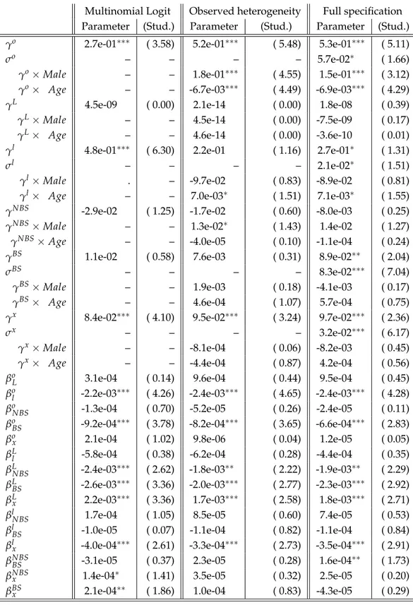
Table 4: Mixed Logit Parameters: Quadratic Utility
Multinomial Logit Observed heterogeneity Full specification Parameter (Stud.) Parameter (Stud.) Parameter (Stud.) γo 2.7e-01∗∗∗ ( 3.58) 5.2e-01∗∗∗ ( 5.48) 5.3e-01∗∗∗ ( 5.11)
σo – – – – 5.7e-02∗ ( 1.66)
γo×Male – – 1.8e-01∗∗∗ ( 4.55) 1.5e-01∗∗∗ ( 3.12) γo× Age – – -6.7e-03∗∗∗ ( 4.49) -6.9e-03∗∗∗ ( 4.29) γL 4.5e-09 ( 0.00) 2.1e-14 ( 0.00) 1.8e-08 ( 0.39)
γL×Male – – 4.5e-14 ( 0.00) -7.5e-09 ( 0.17)
γL× Age – – 4.6e-14 ( 0.00) -3.6e-10 ( 0.01)
γl 4.8e-01∗∗∗ ( 6.30) 2.2e-01 ( 1.16) 2.7e-01∗ ( 1.31)
σl – – – – 2.1e-02∗ ( 1.51)
γl×Male . – -9.7e-02 ( 0.83) -8.9e-02 ( 0.81)
γl× Age – – 7.0e-03∗ ( 1.51) 7.1e-03∗ ( 1.55) γNBS -2.9e-02 ( 1.25) -1.7e-02 ( 0.60) -8.0e-03 ( 0.25)
γNBS×Male – – 1.3e-02∗ ( 1.43) 1.4e-02 ( 1.27)
γNBS×Age – – -4.0e-05 ( 0.10) -1.1e-04 ( 0.24)
γBS 1.1e-02 ( 0.58) 7.6e-03 ( 0.31) 8.9e-02∗∗ ( 2.04)
σBS – – – – 8.3e-02∗∗∗ ( 7.04)
γBS×Male – – 1.9e-03 ( 0.18) -4.1e-03 ( 0.17)
γBS× Age – – 4.6e-04 ( 1.07) 5.7e-04 ( 0.75)
γx 8.4e-02∗∗∗ ( 4.10) 9.5e-02∗∗∗ ( 3.24) 9.7e-02∗∗∗ ( 2.36)
σx – – – – 3.2e-02∗∗∗ ( 6.17)
γx×Male – – -8.1e-04 ( 0.06) -8.2e-03 ( 0.45)
γx× Age – – -4.4e-04 ( 0.87) 4.2e-04 ( 0.56)
βoL 3.1e-04 ( 0.14) 9.6e-04 ( 0.44) 9.5e-04 ( 0.45) βol -2.2e-03∗∗∗ ( 4.26) -2.4e-03∗∗∗ ( 4.65) -2.4e-03∗∗∗ ( 4.28) βoNBS -1.3e-04 ( 0.70) -5.2e-05 ( 0.26) -2.4e-05 ( 0.11) βoBS -9.2e-04∗∗∗ ( 3.78) -8.2e-04∗∗∗ ( 3.65) -6.6e-04∗∗∗ ( 2.83) βox 2.1e-04 ( 1.02) 9.8e-06 ( 0.04) 1.2e-05 ( 0.05) βLl -5.8e-04 ( 0.38) -6.2e-04 ( 0.28) -4.4e-04 ( 0.35) βLNBS -2.4e-03∗∗∗ ( 2.62) -1.8e-03∗∗ ( 2.22) -1.9e-03∗∗ ( 2.29) βLBS -2.6e-03∗∗∗ ( 3.36) -2.0e-03∗∗∗ ( 2.77) -2.3e-03∗∗∗ ( 2.92) βLx 2.2e-03∗∗∗ ( 3.36) 1.7e-03∗∗∗ ( 2.58) 1.8e-03∗∗∗ ( 2.71) βlNBS 1.7e-04 ( 1.05) 8.5e-05 ( 0.60) 7.4e-05 ( 0.53) βlBS -1.0e-05 ( 0.07) -1.1e-04 ( 0.82) -1.1e-04 ( 0.84) βlx -4.0e-04∗∗∗ ( 2.61) -3.3e-04∗∗∗ ( 2.73) -3.5e-04∗∗∗ ( 2.91) βNBSBS -3.1e-05 ( 0.37) 2.3e-05 ( 0.28) 1.6e-04∗∗ ( 1.73) βNBSx 1.4e-04∗ ( 1.41) 3.5e-05 ( 0.32) 2.5e-05 ( 0.20) βBSx 2.1e-04∗∗ ( 1.86) 1.0e-04 ( 0.83) -4.3e-05 ( 0.29)
Table 4: Mixed Logit Parameters: Quadratic Utility (Continued)
Multinomial Logit Observed heterogeneity Full specification Parameter (Stud.) Parameter (Stud.) Parameter (Stud.) βo -4.3e-04 ( 0.71) -7.3e-03∗∗∗ ( 4.05) -9.3e-03∗∗∗ ( 4.02) βo×Male – – -4.2e-03∗∗∗ ( 3.31) -3.8e-03∗∗∗ ( 2.72) βo× Age – – 2.0e-04∗∗∗ ( 4.72) 2.1e-04∗∗∗ ( 4.51)
βL 1.1e-03 ( 0.13) 5.3e-03 ( 0.39) 4.3e-03 ( 0.52)
βL×Male – – -1.8e-03∗∗ ( 1.81) -1.8e-03∗∗ ( 1.84) βL× Age – – -8.6e-05∗ ( 1.63) -7.6e-05∗ ( 1.56) βl -1.7e-03∗∗∗ ( 6.43) -7.1e-04 ( 0.91) -8.9e-04 ( 1.08)
βl×Male – – 4.4e-04 ( 0.90) 4.0e-04 ( 0.86)
βl× Age – – -2.8e-05∗ ( 1.41) -2.8e-05∗ ( 1.47) βNBS -7.1e-05∗ ( 1.59) -6.6e-05 ( 0.65) -2.7e-04∗∗ ( 2.20)
βNBS×Male – – -6.2e-06 ( 0.12) -3.5e-05 ( 0.61)
βNBS× Age – – 5.4e-07 ( 0.30) 3.3e-06∗ ( 1.57)
βBS -1.8e-04∗∗∗ ( 3.41) -9.3e-05 ( 0.89) -3.3e-04 ( 1.12)
βBS×Male – – 5.5e-05 ( 1.13) 1.4e-04 ( 0.98)
βBS× Age – – -1.9e-06 ( 1.07) -6.9e-06 ( 1.06)
βx -2.1e-04∗∗∗ ( 2.88) -1.9e-04∗∗ ( 1.91) -1.5e-04 ( 1.16)
βx×Male – – 2.9e-06 ( 0.07) 7.2e-05 ( 1.26)
βx× Age – – 1.2e-06 ( 0.77) -2.7e-06 ( 1.10)
ψ 4.6e-01∗∗∗ ( 6.41) 4.6e-01∗∗∗ ( 6.42) 4.6e-01∗∗∗ ( 6.28)
Log-Likelihood -4057.0 -3969.9 -3562.6
Legend.Significance levels:∗∗∗10%,∗∗5%,∗∗∗1%.
Note.ML estimation of the model on the sample of pediatricians (N=819 observations). The left-hand side provides point estimates and standard errors of the Multinomial Logit model that includes only parameters from the quadratic function defined over practice variables. Observable heterogeneity is added in the model displayed in the middle of the table. The right-side includes unobserved heterogeneity through random coefficients, assumed normally distributed.
The discrete approach to estimating labour supply models requires the marginal utility of con-sumption to be positive at all chosen points along the budget constraint van Soest (1995). This requirement is satisfied for 86% of observations in the model with observed heterogeneity. It is satisfied for 85% of the observations in the multinomial-logit model (with no heterogeneity) and for 60% of the observations in the model with both observed and unobserved heterogeneity. In the interests of selecting a model that best fits the data, while respecting theoretical restrictions, we con-centrate on the version of the model with observed heterogeneity. Note, we choose this specification in spite of the fact that the likelihood function increased substantially (from -3969 to -3562) upon the introduction of unobserved heterogeneity. This reflects the tradeoff between fitting the sample data