Échevin : Université de Sherbrooke and CRCELB
damien.echevin@usherbrooke.ca
Fortin : Université Laval, CIRPÉE and CIRANO
bernard.fortin@ecn.ulaval.ca
This article was partly written while Fortin was visiting the University Paris I Panthéon-Sorbonne. We gratefully acknowledge Marie Connolly Pray, David Haardt, Nicolas Jacquemet, Pierre-Thomas Léger, as well as participants at CAE conference, SCSE meeting and Ottawa University Department of Economics seminar for their useful comments and suggestions. We acknowledge research
Cahier de recherche/Working Paper 11-12
Physician Payment Mechanisms, Hospital Length of Stay and Risk of
Readmission: a Natural Experiment
Damien Échevin
Bernard Fortin
Abstract:
We provide an analysis of the effect of physician payment methods on their hospital
patients’ length of stay and risk of readmission. To do so, we exploit a major reform
implemented in Quebec (Canada) in 1999. The Quebec Government introduced an
optional mixed compensation (MC) scheme for specialist physicians working in hospital.
This scheme combines a fixed per diem with a reduced fee for services provided, as an
alternative to the traditional fee-for-service system. We develop a simple theoretical
model of a physician’s decision to choose the MC scheme. We show that a physician
who adopts this system will have incentives to increase his time per clinical service
provided. We demonstrate that as long as this effect does not improve his patients’
health by more than a critical level, they will stay more days in hospital over the period.
At the empirical level, using a large patient-level administrative panel data set from a
major teaching hospital, we estimate a model of transition between spells in and out of
hospital analog to a difference-in-differences method. The model is based on a two-state
Mixed Proportional Hazard approach. We find that the hospital length of stay of patients
treated in departments that opted for the MC system increased on average by 10.8%
(0.71 days). However, the risk of readmission to the same department with the same
diagnosis does not appear to be overall affected by the reform.
Keywords: Physician payment mechanisms; Mixed compensation; Hospital length of
stay; Risk of re-hospitalisation; Duration model; Natural experiment.
1
Introduction
Most empirical studies on physicians responses to various payment mechanisms focus on their activities as measured by their volume of services, their hours of work, or their productivity. In general, this research does provide evidence that these choices are influenced by physician remu-neration schemes. See, among others, Gaynor and Pauly (1990), Hemenway, Killen, Cashman, Parks, and Bicknell (1990), Hurley, Labelle, and Rice (1990), Ferrall, Gregory, and Tholl (1998), Barro and Beaulieu (2003), Hadley and Reschovsky (2006), Devlin and Sarma (2008), and Du-mont, Fortin, Jacquemet, and Shearer (2008). However, very few studies have analyzed the impact of alternative methods of physician remuneration on their hospital patients’ length of stay (LOS) and the risk of their re-hospitalisation post-discharge.1
This is unfortunate for at least three reasons. Firstly, for a given diagnosis, outcomes such as LOS in hospital are potentially verifiable, albeit imperfect, measures of inputs that may affect specialists’ quality of service (Chalkley and Malcomson 2000). For instance, an increase in LOS in hospital may reflect more time spent by a specialist to better identify the nature of his patient’s health problem and to improve the quality of treatment. Of course, an increase in LOS in hospital may just reflect the fact that specialists spend more time on nonclinical activities (e.g., teaching, administrative tasks and research) and less time on clinical activities. In this case, one should not expect an increase in the quality of treatment at least in the short run, ceteris paribus. Secondly, the risk of hospital re-hospitalisation post-discharge to the same department is a natural measure of adverse outcome and is often used as a proxy for morbidity (e.g., Cutler 1995). Therefore, one may expect that a longer LOS in hospital, as long as it leads to better service quality in hospital, will reduce the risk of re-hospitalisation post-discharge. Finally, LOS in hospital is generally con-sidered as a major determinant of hospital costs per patient, while hospitalisations account for a large portion of total health care costs, even if they are a relatively rare occurrence.2 Note however that an increase in LOS in hospital is likely to reduce alternative care costs, given the potential
1
One exception is Hutchinson, Birch, Hurley, Lomas, and Stratford-Devai (1996) who analyzed the impact of primary care physician payment mechanisms on hospital utilization rates among patients in Ontario. They found that capitation payment, with an additional incentive payment to encourage low hospital utilization rates, did not reduce hospital use. One limitation of the research is the small number of physicians (39) whose method of payment was converted from fee-for-service to capitation over the period.
2
This is one reason why the prospective payment system (PPS) was introduced for Medicare in 1983 in the U.S. Under the PPS, the federal government reimbursed hospitals a fixed price for each patient treated (based on his diag-nosis) that is independent of the actual costs of treatment (in contrast with the previous cost reimbursement method). It was expected that the PPS system would introduce strong incentives on hospitals to keep costs down by reducing, among others, LOS in hospital. However, there was also fear that such a system could reduce the quality of services in hospital and may result in worse outcomes (e.g., Cutler 1995).
substitution between hospital and post-hospital care (e.g., convalescent home, home care).
This paper attempts to partly open the black box of the impact of physician payment mech-anisms on LOS in hospital and the risk of re-hospitalisation post-discharge to the same depart-ment with the same Diagnosis-Related-Group (DRG).3 To do so, we exploit a major reform of physician-payment mechanisms implemented in the Province of Quebec (Canada) by the Quebec Government. This reform consisted in introducing an optional mixed compensation system (MC) for specialists working in hospital, as an alternative to the traditional fee-for-service (FFS) sys-tem.4 The MC system combines a fixed per diem with a discounted (relative to the FFS system) fee for services provided. Upon the introduction of the MC system, each department voted on its adoption, switching to the MC system only if the vote passed unanimously.5 In 2008, close to 50% of all specialists had opted for this system in Quebec.
In economic terms, the two main objectives of this reform can be stated as follows. Firstly, it was aimed at reaching a more efficient quantity-quality trade-off in health care provided by spe-cialists. Since the MC system introduces a per diem independent of the number of clinical services provided and strongly reduces the fees per service (at about 41% of the average fee), specialists who opt for MC may have incentives to reduce their supply of clinical services. This effect may improve the efficiency in health-care allocation of resources as long as the volume of clinical ser-vices provided under FFS is excessive. For instance, a FFS specialist may have incentives to abuse his role as a medical adviser and multiply the number of non-necessary services in hospital to ad-vance his own economic self-interests. This phenomenon of physician-induced-demand (PID) may occur when an asymmetry of information exists between provider and consumer in the physi-cians service market.6 On the other hand, physicians who choose the MC system are expected to
3The DRG system classifies hospital cases expected to have similar hospital resources use into approximately 500
groups DRGs are assigned by an algorithm based on the International Statistical Classification of Diseases and Related Health Problems (ICD) diagnosis codes, Current Procedural Terminology (CPT) codes, age, gender, and the presence of complications or co-morbidities. An example might be the group of females aged 55 and older with a Breast Cancer diagnosis, a Mastectomy procedure code and an osteoporosis diagnosis (comorbidity).
4
In Quebec, as in each of the Canadian provinces and territories, all physicians work within a universal public Health Care System.
5
The MC system is available only for activities completed in health establishments (mainly hospitals). Services provided within private clinics continue to be generally paid under the FFS system. Also, there are restrictions on the number of per diems a physician can claim and the time-period during which he can claim them. Half per diems are claimed on a 3.5-hour basis. The maximum number of half per diems that a physician can claim during a two-week period is 28 and these can only be claimed Monday to Friday between 7AM and 5PM. Once the maximum number of per diemsis reached, or when a physician works outside the per-diem claimable hours, he is paid on the FFS basis. See Dumont, Fortin, Jacquemet, and Shearer (2008) for more detailed description of the reform.
spend more time per clinical service provided, as they are paid more in time and less in clinical services. This effect may improve the quality of clinical services.7 All in all, these predictions are consistent with Dumont, Fortin, Jacquemet, and Shearer (2008) according to which the 1999 Quebec reform induced specialists who switched to MC to reduce their volume of clinical services by 6.15% while increasing their average time spent per clinical service by 3.81%. These results suggest a potential quality-quantity substitution.
A second objective of the reform was to improve efficiency in the allocation of time between clinical and nonclinical activities. Since the latter are not remunerated under the FFS system, they are likely to be neglected. As long as they are included in the per diem under MC,8this system is likely to stimulate these activities. Results from Dumont, Fortin, Jacquemet, and Shearer (2008) also confirm this prediction. Specialists who adopted MC increased their time spent on admin-istrative and teaching tasks (activities not remunerated under FFS) by 7.92% while they reduced time spent on clinical activities by 2.57%. Thus, the reform may favour a more efficient allocation of tasks within departments that adopted a MC system.9
We assess the effects of the introduction of the 1999 Quebec reform on both LOS in hospital and the risk of re-hospitalisation of patients treated in departments that opted for the MC system (average treatment effects on the treated). Our contribution is both theoretical and empirical. At the theoretical level, we provide a static model that shows that, under realistic assumptions, the reform induces a physician who opts for the MC system to perform less clinical services per unit of time. Therefore, he will spend more time per clinical service. Assuming for simplicity fixed on-the-job leisure and nonclinical activities, this is likely to increase the quality of services. How-ever, as long as this effect does not reduce the required volume of services to treat a patient by less than a critical level, his time spent in hospital will increase over the period. Of course, since given
altruism are forces that may limit PID. Note also that waiting lists to see specialists are very long in Quebec. Under these circumstances, FFS specialists’ incentives to induce demand are likely to be reduced. Literature on PID is plentiful but empirical evidence is mixed. See McGuire (1997) for a recent survey.
7
Ma and McGuire (1997) suggest the use of average time spent per service as a proxy for the intensity or quality of treatment provided by the physician. Of course, time spent per service is an imperfect measure of quality − physicians may simply be taking longer breaks between services, or spending more time with patients without affecting health outcomes.
8
The per diem only applies to certain activities, principally time spent on administration, teaching and seeing patients, the most notable exclusion being time spent on research. Research activities are typically paid by the hospital where they take place, or through government grants.
9
A third objective of the reform was to improve horizontal equity between specialists with different behaviours in terms of clinical and nonclinical activities. For instance, the pay gap between specialists who mainly do clinical tasks and those who do a higher proportion of administrative tasks is likely to be reduced in departments that opted for MC.
that our model is static and under certainty, one cannot theoretically decompose this impact on a patient’s LOS in hospital and his risk of re-hospitalisation. However, economic intuition suggests that, in MC departments, the patient’s LOS in hospital is likely to increase (more time per service in hospital) but the risk of re-hospitalisation post-discharge may decrease (higher quality of ser-vices received when hospitalized). Besides, if the reform only has an effect on the reallocation of tasks toward less clinical and more nonclinical activities in MC departments, the LOS in hospital is expected to increase, but with little impact on the frequency of re-hospitalisation. All in all, one expects the reform to increase LOS in hospital in MC departments while its impact on the risk of re-hospitalisation is expected to be negative or zero. An empirical analysis is required to test these predictions.
As we cannot exploit a randomized experiment, our methodology uses a quasi-experimental design based on a two-state duration model analog to a difference-in-differences approach. The control groups are defined by departments that remained within the FFS system. We make clear the assumptions we adopt to allow our empirical approach to identify the impact of the reform, given that the decision of a department to move to the MC system is endogenous. To estimate the model, we take advantage of a unique administrative patient-level dataset from a major teach-ing hospital in Quebec (Sherbrooke University Hospital Center).10 One advantage of using one hospital is that it allows us to control for hospital unobservable characteristics and the social envi-ronment that may affect the impact of covariates.
At the empirical level, we estimate a reduced-form transition model of patients’ hospitalisa-tion and re-hospitalisahospitalisa-tion post-discharge. We use a Mixed Proporhospitalisa-tional Hazard (MPH) approach as developed by Lancaster (1979) and extended by Meyer (1990) and Han and Hausman (1990) to allow for flexible baseline hazard. We estimate the analog of a difference-in-differences model within our MPH approach. In particular, fixed effects per department are introduced to account for unobservable characteristics that may explain their decision to adopt or not the MC scheme and that could be the source of a potential selectivity bias. Such a bias stems from the fact that the incentive to move to MC is likely to be stronger in departments where physicians favour longer lengths of stay in hospital. We also include a number of covariates (e.g., patient’s gender, age, time polynomial, and 365 diagnosis dummies) to control for confounding variables. The number of observations include as many as 144,510 spells in hospital and 125,291 spells outside hospital.
10
Sherbrooke is the 6th largest city in Quebec with a population of 155, 583 people in 2010. Sherbrooke University Hospital Center, a 682-bed multi-facility hospital, is the only university and regional hospital in that region of Quebec.
Our empirical results suggest that the length of stay increased on average by 10.8% (0.71 days) in departments that moved to a MC system (average treatment effect on the treated). How-ever, the risk of re-hospitalisation does not appear to be affected by the reform, at least not at the global level. The positive impact of the reform on time spent in hospital by patients treated in MC departments is consistent with our static model. The absence of effect on the probability of re-hospitalisation at the global level may be partly explained by the fact that the reform does not influence patients’ health in hospital. The reform may also induce MC physicians to reallocate their time toward more nonclinical activities (teaching and administration) but less clinical activ-ities, thus increasing the length of stay of patients in hospital but with little effect on the risk of re-hospitalisation.
The paper is structured as follows. Section 2 presents a theoretical model of the impact of a mixed payment system on the length of stay. Data are presented in Section 3. Section 4 introduces the econometric framework for the estimations. Section 5 presents the results. The last section concludes.
2
Theoretical Model
The determination of the average duration and frequency of hospitalisation is a result of a complex process of interaction between patient characteristics, social environment, hospital characteristics, firms offering covered post-hospital care, (public and private) insurers, and medical practice (see Picone, Wilson, and Chou 2003). However, given the aims of this study and the nature of our data, we focus on medical practice, assuming the characteristics and behaviour of all the other agents to be constant .11 In particular, the patients are assumed to be passive and to have no influence on their number of days spent in hospital over the period.12 To motivate our empirical approach,
we present a simple static model of the impact of the introduction of an optional MC system on a physician’s medical practice and, as a consequence, on the average number of days spent by his patients in hospital over the period. For simplification sake, our model ignores the presence of physician-induced demand (PID).
11Most studies on length of stay have focused primarily on the effects of patient and hospital characteristics. See
Ellis and Ruhm (1988) for a theoretical model of hospital length of stay along these lines.
12
In the context of excess health care demand observed in Quebec, it is plausible to suppose that the patients have no power to negotiate for health services in the hospital.
Consider a representative physician who works in a hospital department and spends his work-ing time performwork-ing clinical services.13 His preferences are represented by a standard utility func-tion given by
U = U (X, e, D), (1)
where X represents his total consumption, e his effort at work, and D his number of working days. The utility is twice-differentiable, strictly quasi-concave, increasing with X and decreasing with e and D. The physician faces the following simple budget constraint:
X = pS + wD + y, (2)
where S is a Hicksian aggregate of his clinical services, p is the corresponding fee per service, w is the per diem and y is his nonlabour income. In this model, there are two prices, one for the services performed, and one for the days worked. Under a FFS system, p > 0 and w = 0; under a wage compensation system, p = 0 and w > 0; and under a mixed compensation (MC) system, p > 0 and w > 0. Under a public health system such as the one prevailing in each Canadian province, prices are exogenous to the physician as they are determined by the government. The physician’s effort, e, is approximated by the volume of his services per working day. Inversely, time spent per service, 1/e, can be taken as a proxy for the quality of services − changes in which are a valid measure of changes in time spent providing services as long as on-the-job leisure is fixed. The (Cobb-Douglas) production function for clinical services is thus given by S = eD. Substituting in (2), the budget constraint becomes:
X = peD + wD + y (3)
The physician is assumed to choose his effort e (or, equivalently, the quality of his services, 1/e), his number of working days D and his consumption X which maximize his utility function (1) subject to his budget constraint (3).
The optimization program to be solved is not standard since the budget constraint is nonlinear in effort e and the number of days D. The standard approach to solve this problem (e.g., Becker and Lewis 1973, Blomquist 1989) is to linearize the budget constraint at the optimum. From this linearization, one can define the virtual (or local) price of effort as pve = pD, the virtual price of
13
working days as pvD = pe + w, and the virtual nonlabour income as yv = y − peD. A key feature of this analysis is that the virtual price of effort increases with the number of working days, the virtual price of working days increases with effort, and the virtual non-labour income decreases with effort and working days. Therefore a change in p or in w will in general affect both virtual prices and the virtual nonlabour income, since e and D are choice variables. Assuming a unique interior solution to the program, the structural (Marshallian) equations for effort and working days supplied are given by:
e = e(pD, pe + w, y − peD) and (4)
D = D(pD, pe + w, y − peD). (5)
Now let us first assume that the compensation system in place at the start is a FFS. The impact of the introduction of an optional MC that reduces the FFS by ∆p and introduces a per diem, w, on physician’s effort, can be approximated by differentiating the structural equations (4) and (5), and by using Slutsky equations that decompose virtual price effects into substitution and income effects.14 Note that symmetry and positive semidefinitiveness of the Slutsky matrix impose stan-dard restrictions on substitution effects.15An important point here is that since the MC is optional, the physician will opt for the MC system only if it increases his earnings at constant behaviour, i.e.,only if e0∆p + w > 0, where the subscript 0 denotes the FFS initial situation.16 This means
that a physician will adopt MC if his effort e0is smaller than w/(−∆p).
One obtains:
∆e ≈ Ω−1[A∆p + Bw + CD(e0∆p + w)] if e0∆p + w > 0 (6)
= 0 otherwise
14
The Slutsky decompositions are: e1 =ee1+ ee3, e2 =ee2+ De3, D1 = eD1+ eD3, and D2 = eD2+ DD3, where ∼ stands for a compensated effect.
15
The Slutsky restrictions are :ee1≥ 0, fD2≥ 0,ee2 = eD1, andee1De2−ee22≥ 0. 16
This is strictly correct when changes in p and w are infinitesimal. With finite changes, one must compare the physician’s (indirect) utility levels under MC and FFS systems.
where Ω = 1 − (ee1De2−ee22) − 2ee2p, A = (ee1De2−ee2 2)ep + e e1D +ee2e, B = (ee1De2−ee2 2)p + e e2, and C = (ee1D3−ee2e3)p + e3.
In (6), Ω−1is the fundamental non-linearity scalar. It transforms linear income and substitu-tion effects into nonlinear ones (see Blomquist 1989, p.282). It is easily shown that Ω is positive if the product of the own compensated elasticities of effort and working days supplied is smaller than e0p/(e0p + w), which is greater than 1. In the following, we will assume that this is the case since
almost all estimated (compensated) labour supply elasticities are smaller than 1 (see Blundell and MaCurdy 1999).
The first two expressions within the brackets on the right-hand side of (6) represent the substi-tution effects respectively associated with the change ∆p in the fee and the introduction of the per diemw, and the third expression represents the income effect. Without additional assumptions, the impact of the MC on the physician’s effort is ambiguous. However under plausible sufficient assumptions, it is possible to sign it.
Firstly, assume that effort and working days are net substitutes in the physician’s preferences (ee2 ≤ 0) and that leisure at work and leisure outside work are normal goods (i.e., e3 ≤ 0 and D3 ≤ 0). In this case, the income effect of the reform is negative (since C ≤ 0). This result
is intuitive: the physician who opts for MC benefits from an increase in his income (at constant behaviour) which induces him to reduce his effort at work. Second, under the assumption that the own compensated elasticity of effort exceeds its corresponding cross elasticity (in absolute value), one has A ≥ 0. Therefore, the substitution effect of the reduction in the fee (∆p ≤ 0) induces the physician to reduce his effort. Again, this result is intuitive: with a decrease in the piece rate per service, the physician will perform less services per day.
The substitution effect of the introduction of the per diem is more difficult to sign. However, one can easily show that if the cross compensated elasticity of effort (in absolute value) exceeds the product of the own compensated elasticities of effort and working days, which is not an im-plausible assumption, one has B ≤ 0. In this case, the substitution effect of the per diem on effort
will be negative. The intuition of this result is also clear: the per diem induces the physician to substitute working days for effort. In short, under plausible assumptions, both income and substi-tution effects induce the physician to reduce his effort at work under MC.
We should now examine the following question: what is the relationship between the physi-cian’s effort and the average number of days spent by his patients in hospital? To provide an answer to this question, let us first define the following variables:
a ≡ S
N, the average volume of services per patient, and (7)
d ≡ D
N, the average number of days in hospital per patient, (8)
where N is the number of patients treated by the physician over the period. Therefore, one has d = S/DS/N = a/e. Now, we assume that the patient’s health improves when a physician spends more time to perform it. In that case, the average volume of services per patient necessary to treat health problems will increase with e, the volume of services performed by the physician per working day.17 Since we assume no PID, it is realistic to assume that the physician provides the number of services just necessary to treat his patients. We thus have:
a = f (e), with f0(e) ≥ 0. (9)
Substituting (9) in d = a/e, on obtains:
d = f (e)
e . (10)
Differentiating (10), the average change in time spent in hospital by patients treated by a physi-cian who opts for MC can be approximated by:
∆d d0 ≈ (ηa,e− 1) ∆e e0 , (11)
where ηa,eis the elasticity of a with respect to e evaluated at the initial FFS situation, 0.18
Equation (11) makes clear that the introduction of a MC system yields two opposite effects on d, the average time spent in hospital by patients. On the one hand, a physician who adopts the MC
17We assume that the volume of beds attributed to a physician per working day is exogenous as it is determined by
the hospital. Therefore e is proportional to the volume of services per bed per working day.
18Using (8) and (10), the number of patients N is given by N = D
d =
De f (e).
system reduces his volume of services per working day (∆ee
0 < 0). This effect tends to increase d,
ceteris paribus. On the other hand, since e decreases and ηa,e > 0, the patient’s health tends to
increase for a given level of services and therefore less services are needed to treat patients. This effect tends to reduce d. Equation (11) shows that the net effect depends on whether the elasticity of a with respect to e, ηa,e, is smaller or greater than one. As long as the negative effect of the
reform on the volume of services required by patient is not too strong (i.e., ηa,e< 1), the average
time spent by patients treated by MC physicians will increase over the period.
Now we can decompose the average number of days spent in hospital by patients over the period into the product of their average length of stay in hospital, l, and their average frequency of hospitalization, f. Therefore, one has d = lf. However, since our model is static, it cannot sign the impact of the reform on the duration of hospital stay and the frequency of re-hospitalisation. Nevertheless, economic intuition suggests that, in MC departments, patients’ average LOS in hos-pital is likely to increase, at least as long as the positive impact of higher time spent per service provided by physicians is not too strong on patients’ health. One also expects that the risk of re-hospitalisation post-discharge may decrease as long as the patient’s health in hospital improves.
The impact of the reform on the reallocation of tasks toward less clinical and more nonclinical activities in MC departments (ignored for simplicity in the model) must also be taken into ac-count. One should expect that this change in behaviour will increase the average LOS in hospital, but with little impact on the risk of re-hospitalisation. Combining these effects, the reform is likely to increase LOS in hospital in MC departments while its impact on the risk of re-hospitalisation is expected to be negative or zero. Our empirical analysis attempts to test these predictions by estimating a reduced form transition model of hospitalisation and re-hospitalisation analog to a difference-in-differences (DD) approach. This model allows us to evaluate the impact of the re-form on the average LOS in hospital and the risk of re-hospitalisation of patients treated in MC departments.
3
Data Description
The data concerns patients’ hospitalisations in a teaching hospital (Sherbrooke University Hospi-tal Center). Only patients who stayed in hospiHospi-tal one day or more are considered in the data. Each patient discharged from hospital was registered in the database over a period of 9 years (1999-2007) with their precise time of admission to hospital, age, gender and department of admission,
as well as the time when the patient left the hospital, department and Diagnosis-Related-Group (DRG) when leaving.
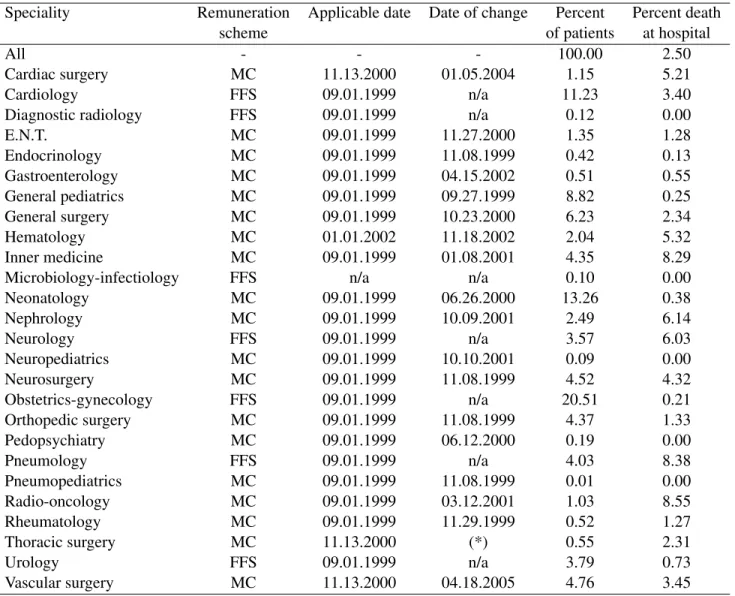
Due to problems of access to data, we could not use a sample period starting before 1999. One could argue that this reduces the period of observation to a small number of months before the reform, since the latter was implemented on September 1st 1999, while our sample period starts on January 1st 1999. Note however that the average LOS in hospital is 6.3 days. Therefore, there is still a large number of spells in hospital (13,445 visits) within this time interval. Also, not all treated departments moved to the MC system in September 1999. The first move to MC occurred on September 27th 1999 and the last on April 18th 2005 (see column 3, Table 1). In fact, most treated departments (12 over 19) chose to opt for MC in 2000 or later. This corresponds to two thirds of all spells in treated departments. One reason why they did not make the move at the start of the reform is that the applicable date at which a speciality could adopt MC (see column 3, Table 1) was negotiated at the provincial level by the government and each medical specialist associa-tion. A second reason is that departments were waiting for information or recommendations from their own association.
Each patient leaving the hospital was registered over a 9-year period, from January 1st 1999 to December 31st 2007. Hence, this data allows us to calculate the complete LOS in hospital and the length of stay out of hospital for each patient over this period. As regards spells in hospital, there is no left-censoring since the time of admission is available for all patients. However, right-censoring exists since we do not have information on the duration of hospital spells in the case of individuals who were still hospitalized on December 31th 2007. Moreover, 2.5% of patients (see last column of Table 1) died in hospital and their spells are therefore censored.19Also, there is no left-censoring for spells outside of hospital after a first period of hospitalisation within the sample period. However, right-censoring is present for two reasons. Firstly, some individuals were out of the hospital at the end of the sample period. Secondly, since we focus on returns to hospital in the same department with the same DRG, spells ending in hospital but in another department or DRG are considered censored. Our econometric model takes these right-censored spells into account.
Table 2 summarizes descriptive statistics over the sample period. As mentioned above, the LOS in hospital is 6.3 days on average (ignoring right-censoring). Its median value is 3 days; the 25th percentile is 2 days while the 75th percentile is 7 days. The length of stay outside of hospital
is 455.9 days on average (ignoring right-censoring), with 80% of the population going back to hos-pital after staying 10 (10th percentile) to 1262 days (90th percentile) out of hoshos-pital. The number of spells in hospital per patient is on average 1.6, with a 25th percentile of 1 and a 75th percentile of 2. 90% of the population return to the hospital 3 times or less over the period considered. If we consider patients returning to hospital, the average number of spells in hospital is 2.9, whereas this average is 1.7 when considering individuals coming back to the same department. The average number of spells in hospital falls to 1.3 for individuals returning to the same DRG. The age of patients is on average 40.9, with 75% being less than 66 years old, and the percentage of males being 45.1%.
Since the last move to the MC system occurred in April 2005, we chose to restrict our obser-vation window to the period from January 1999 to April 2006. Given this choice, spells in hospital are no longer right-censored, except for episodes lasting more than 8 months (they are very few) or censored by the death of the patient (they represent 2.5% of the sample; see table 1).
4
Empirical Framework
In this section, we present a two-state transition model which allows to identify the impact of the reform on two outcomes for hospital departments that opted for the MC system (the treatment groups): patients’ exit rates from hospital and their risk of re-hospitalisation to the same depart-ment and the same DRG. These outcomes can also be expressed in terms of the corresponding average duration in and out of the hospital. Our approach extends the model developed by Fortin, Lacroix, and Drolet (2004) to account for the presence of many treatment and control groups.
We assume that two states are possible for a patient: (i) in hospital (s = 1) and (ii) out of hos-pital (s = 2). Here, two important remarks are in order. Firstly, as suggested by Picone, Wilson, and Chou (2003), we also implemented a competing risks model with several post-hospital des-tinations for a patient in hospital. Given the administrative nature of our data, we could consider only two mutually exclusive destinations: (a) death in the hospital and (b) other out of the hospital destinations. However, in no specification did the reform have any overall effect on death in the hospital destination. Therefore, we have decided to restrict our analysis to a two-state model with spells with death in the hospital assumed to be censored. Secondly, with regards to spells out of hospital, we considered a competing risk approach to deal with destination in hospital but not in the same department or DRG. However, this did not change our results in any significant way.
Therefore, these destinations are also considered censored.
Our model contains many treatment groups and the time at which they are treated varies across groups. A department is a treatment group if it moves to the MC system within the sample pe-riod.20 Otherwise, it is a control group. There are Ks(with K1 = 23 and K2 = 22)21departments
considered in the hospital (k = 1, ..., Ks), of whom the first Rs’s (with R1 = 15 and R2 = 14)
opted for the MC scheme within the sample period.
Consider a patient i, who has occupied a state s for a duration t, in his spell j, in the department kij (it refers to the last department where he was hospitalized if he is out of the hospital), at
calendar time τij (= τij(t)), and with xij (= xij(t)) time-varying observed characteristics.
The calendar time at which a treated department k switched to MC is given by ck. We assume a
flexible mixed proportional hazard (MPH) model based on Meyer (1990) approach. The model is time-continuous but interval-censored, that is, not directly observed, but observed to fall within a known interval (i.e., one day). The individual’s conditional hazard (or exit rate) function for each state s is given by:
λs(t|zsij(t), νijs) = exp(zijs(t))λs0(t)νijs, s = 1, 2, (12) with zijs(t) = Ks X k=1 αs1kI(k = kij)+ Rs X k=1 αs2kI(τij ≥ ck)+P 0 (τij)γs+ Rs X k=1 βksI(k = kij)I(τij ≥ ck)+x 0 ijδs, (13) where I(A) is an indicator function equal to 1 when A is true and 0 otherwise, and P(τij) is a
polynomial function of time. Eq. (12) specifies the hazard rate as the product of three compo-nents: a regression function, exp(zijs), that captures the effect of observed explanatory variables, a baseline hazard, λs0(t), that captures variation in the hazard over the spell, and a random term, νijs, that accounts for the patient’s and his treating doctor(s)’ unobserved characteristics.22
The regression function (in log) is given by eq. (13). It corresponds to a standard DD
ap-20
No MC department moved back to the FFS scheme over the period.
21
The total number of departments is 26 (see Table 1). However, given the very low number of patients in neuro-pediatrics, radio-oncology, and pneumopediatrics in our sample period, these departments have been removed from all our estimations. Moreover, given the small number of returns in neonatology, this department has also been removed from our re-hospitalisation estimations.
22
proach translated into a regression equation, when there are many treatment and control groups. The first expression in the right-hand side of (13) introduces department-specific fixed effects. They take into account departments’ time-invariant unobservable characteristics. The second ex-pression takes into account a hazard break common to all departments, after each time cka treated
department k switches to MC. The third expression is a polynomial function of time which allows for a nonlinear trend in hazard that is common to all departments.The fourth expression accounts for the change in the hazard (over the common break and trend) that occurs for each treated de-partment k (with k = 1, ..., Rs), after the time ck it switches to MC. The βks’s coefficients are
interpreted as the impact of the reform on treated departments (the average effect of treatment on the treated). Finally, the covariates xij account for patient’s characteristics such as his gender, his
diagnosis (365 dummies) and his age.
The MPH model is nonparametrically identified under standard assumptions including mini-mal variations in covariates and independence between the covariates and the individual random term (see Van den Berg (2001) for a recent survey). The latter assumption raises a number of important issues in our setting. Firstly, our econometric approach must address the selectivity bias associated with departments’ decision to opt for MC. Recall that it is not the physician but the department, by a vote at unanimity, that decides to make such a choice. This endogeneity problem may render difficult the identification of the impact of the reform. For instance, the incentive to move to MC is likely to be stronger in departments where physicians’ treatment approach is to favour longer hospital lengths of stay. This may create a positive bias on the effect of the reform on the duration of spells in hospital. We assume that the department-specific fixed effects take this problem into account. More precisely, a condition for identification is that these effects capture the unobserved common characteristics of physicians’ preferences regarding the change of payment system within a department.23 Secondly, related to the latter point, we suppose that, conditional on department-specific fixed effects, ck is strictly exogenous. This means that the department’s
decision to choose MC at time ckwithin the sample period is independent from the treating
physi-cian’s unobservable characteristics other than those taken into account by his department’s fixed effect.
A related identification issue is whether the βks’s coefficients can be interpreted as the impact of the reform on treated departments. As in the standard DD approach, a basic condition is that,
23
Note that other factors could influence the decision to move to MC –such as the recommendations by specialist associations at the provincial level.
once controlling for common shocks and common time effects across departments, there is no shock other than the reform that affects the treated departments’ outcomes after their adhesion to MC. Also, patients in departments that remained under FFS (control groups) must not be affected by the reform (no general equilibrium effects). Finally, one must assume that patients did not move from one department to another within a same spell because their department opted for the MC system.
In line with the Meyer model, the baseline hazard is modeled as a piece-wise function of time, that is, λs0(t) = λsv for tv ≤ t < tv+1and v = 1, ..., M . It is thus assumed that λs0(t) is constant
within specified duration intervals. This allows for flexibility in the relationship between the spell duration and the hazard rate from a state.
A parametric Gamma function is used for the distribution of the heterogeneity term νijs. We use this parametric function rather than a non-parametric approach for a number of reasons. Firstly, it has been recently proved by Abbring and Van den Berg (2007) that the distribution of unobserved heterogeneity in MPH models converges to a Gamma distribution under realistic assumptions.24 Second, contrary to the Heckman and Singer (1984) (HS) alternative approach which assumes a nonparametric specification of the heterogeneity by introducing an exogenous discrete number of support points, the Meyer model yields an asymptotically normal estimator so that standard large sample inference can be used. Indeed, one basic problem with the HS estimator is that its asymptotic distribution is not known. Monte Carlo simulations by Baker and Melino (2000) have shown that the HS approach provides inconsistent estimates of the MPH model, when the baseline hazard is left fairly free. Thirdly, Han and Hausman (1990) report empirical results indicating that a flexible specification of the hazard function sharply reduces the sensitivity of the estimates to a parametric heterogeneity assumption.
Here a number of important remarks are in order. Firstly, since νijs includes both a patient’s and his treating physician(s)’ unobservable characteristics, we cannot assume that it is invariant across various spells within a same state as in a standard multi-spell model. Indeed, a patient may change physicians from one spell at the hospital to another. Secondly, we ignore for simplicity the presence of dependency between unobserved heterogeneity across spells of a same individual.25 However, we do introduce some dependency across spells by allowing the re-hospitalisation
haz-24
Given the very large number of observations in our data set, the asymptotic properties of our estimators are likely to hold.
25
ard of a patient outside of hospital to be related to his diagnosis in his preceding spell of hospi-talisation. Also, we ignore occurrence and lagged duration dependence (i.e., dependence of the termination probability of the spell in progress on either the number or the duration of previous spells) as well as serially correlated unobserved heterogeneity. Incomplete information regarding previous hospital spells leaded us to adopt this strategy. Also, introducing diagnosis dummies is likely to partly control for these problems. Finally, as discussed earlier, left-censoring of the first spell is not a problem in our panel data, while right-censoring are taken into account in the esti-mations.
5
Results
In what follows, we provide maximum likelihood estimation results from our two-state MPH model.26 In our specifications, we included six time (in days) intervals to account for our flexible baseline hazard in each state. The intervals considered are 0, 1, 5, 10, 15, 20 + in the case of spells in hospital and 0, 10, 50, 100, 500, 1000 + in the case of spells out of hospital. These intervals were chosen based on histograms of spells in each stage. A number of experiments suggest that the impact of other covariates are little affected by changes in the number and the size of these intervals.
As regards the control variables, after a number of experiments, we have introduced a quadratic time polynomial (Trend and Trend2). Introducing higher power levels in time did not change the parameters of interest (i.e., the β’s) in any significant way. Also, a quadratic polynomial in age, a gender dummy and six dummies for the day at which the patient was admitted in the hospital have been included as control variables. In the latter case, one expects that a patient admitted on Saturday or Sunday will stay longer in hospital since medical exams and treatments are usually less numerous during the weekend.
Table 3 provides the parameter estimates of the hazard rate from hospital. We test several specifications of the same model. In the first specification (model 1), we use Gamma hetero-geneity of the error term and do not add DRG dummies. The β coefficients (which measure the average treatment effect on each treated department) are negative for 12 departments/specialities and, among these, significant at the 5% level for 8 departments out of 15 which have moved to
26
MC in our sample. Patients in these 8 departments represent 68.26% of all MC patients in our sample. The coefficients are positive and significant for only two departments (vascular surgery and hematology). Patients in these departments represent 12.4% of all MC patients in our sample. This indicates that the rate of exit from hospital is reduced in most departments that moved to MC. The negative effect varies from 7.6% in general pediatrics to 36.2% in rheumatology.
Interestingly, we find that the variance of the Gamma distribution (θ) is not statistically signifi-cant according to the LR test.27 The rejection of unobserved heterogeneity is a current result in the literature especially in the presence of a flexible parametric representation of the baseline hazard (see Baker and Melino 2000). To analyse the robustness of this result, we re-estimated the model using the Inverse Gaussian distribution. In that case also, we could not reject the null hypothesis that the variance of the distribution is zero. The absence of unobserved heterogeneity problems partly justify our assumption that spells in and out of the hospital are independent.
In model 2, we add the 365 DRG dummies while excluding Gamma heterogeneity.28 The
DRG dummies are jointly significant according to a LR test. Model 2 slightly alters our results. The reform still has a significantly negative impact on the exit rate from hospital on 8 departments out of 15. However, in this specification, it is not positive and significant for any department. The negative effect varies from 7.7% in general pediatrics to 48.4% in rheumatology. This specifica-tion suggests that the reform has increased LOS in hospital for 68.26% of all MC patients in our sample while it has had no influence on LOS for the other patients.
Model 3 provides results from the standard Cox specification (proportional hazard with no unobservable heterogeneity). This model is estimated using partial maximum likelihood so that results are not affected by the functional form of the baseline hazard (nonparametric model). Esti-mates in model 2 and 3 are very similar. This is what we expected since unobserved heterogeneity is rejected in model 2 and that both models allow for flexible baseline hazard. Finally, model 4 yields estimates when imposing the equality of the β coefficients. While a LR test strongly rejects these restrictions (χ2 statistic test= 68), the estimated global β coefficient can be interpreted as a weighted average of the impact of the reform on treated departments. According to results, the
27Note that the test is a boundary test that takes into account the fact that the null distribution is not the usual
chi-squared (with one degree of freedom) but is rather a 50:50 mixture of a chi-chi-squared (degree of freedom = 0) variate (which is a point mass at zero) and chi-squared (degree of freedom = 1). The standard chi-squared test is incorrect since the model with no unobservable heterogeneity is not nested in the model with Gamma heterogeneity.
28When adding both DRG and Gamma heterogeneity, the variance of the Gamma distribution still appears to be not
exit rate from hospital decreased by about 9.5% on average in departments that moved to MC, with this effect being significant at the 1% level.
Looking at other covariates in model 2, we find, as expected, that age has a negative impact on the exit rate from hospital and that starting hospitalisation during the week-end has a negative impact as well. Being a male has a positive impact on the exit rate (presumably due to a higher average opportunity cost in terms of wage earnings and easier substitutability between home and hospital care). The effect of the time trend appears to be negative whereas most post-change de-partment dummies (the α2’s) have a positive impact.
We simulate the impact of the reform on the duration of hospitalisation in Table 4 using Katz and Meyer’s (1990) approach. Relative effects of the change in payment system on expected du-ration and their standard errors are computed using the Delta method. They are estimated for each treated department over the sample period 1999-2006. Relative effects are calculated for each department using model 2 specification and overall using model 4 specification. The simulations use parameter estimates to predict the expected duration of hospitalisation over the sample period, with or without the effect of the change. The simulation procedure states as follows. Firstly, the predicted survivor function is simulated for each patient and each day of hospitalisation and then aggregated for the sample over individuals. Second, the predicted mean duration is calculated by accumulating the aggregate survivor function by day.29 Finally, we estimate the difference be-tween expected durations estimated with and without the change. Relative effect is obtained by dividing the difference by the expected duration estimated without the change.
We find that LOS in hospital has increased by 0.71 days overall in treated departments. This corresponds to a percentage increase of 10.8%. The department of rheumatology experienced the largest impact with an increase in LOS by 3.86 days (or 68.5%) while the general pediatrics department experienced the lowest positive impact with a LOS increase of 0.27 days (or 7.9%). Other specialities such as neonatology and gastroenterology have also experienced low positive and significant impacts on days in hospital. These small increases may partly be explained by the fact that fewer services are provided by these specialists. Moreover, regarding neonatology, the discharge of newborns does not generally depend on the volume of services provided and thus may not be strongly influenced by the reform. For instance, in the case of acute medical problems,
29
Note that the number of days used for this computation should be large enough in order for the procedure to converge.
in order to be discharged, premature infants must know how to feed by themselves and grow; car-diorespiratory stability is also a prerequisite that may only depend on time. On the other hand, the discharges in rheumatology may be more dependent on the volume of services provided.
Table 5 presents the parameter estimates for the risk of re-hospitalisation to the same depart-ment with the same DRG. Model 1 does not include DRG dummies and assumes Gamma hetero-geneity with covariates given by age, age2, gender and a quadratic time trend. Results indicate that the impact of the reform is non significant for 9 departments, positive and significant for four departments (vascular surgery, neurosurgery, inner medicine, and rheumatology), and negative for only one department (endocrinology), out of 14 MC departments.30 This suggests that the reform has increased the re-hospitalisation rates for 25.7% of MC patients and has reduced these rates for 0.76% of them. In this specification, the variance of the Gamma distribution is high and sig-nificantly different from zero, which suggests the presence of relevant unobserved heterogeneity. As expected, age has a positive impact on re-hospitalisation rates over a critical level. Moreover, being a male reduces the risk of re-hospitalisation. Finally, time trend has a negative effect on re-hospitalisation rates but at a decreasing rate.
Model 2 adds DRG dummies while still allowing for Gamma unobserved heterogeneity. In this specification, the impact of the reform is no longer significant for neurosurgery so that the impact of the reform is now not significant for 10 departments. As a consequence, the reform is predicted to increase the re-hospitalisation rate for 17.5% of MC patients. One possible interpre-tation of this result is that the reform induces changes in practice patterns for MC physicians in some departments. Given that their patients’ LOS increases with the reform, they may now prefer to re-hospitalize some of their patients (for a given diagnosis) rather than to treat them within only one hospital spell. Another interpretation is that MC physicians’ on-the-job leisure increases with the reform and this favours re-hospitalization as quality of their clinical services in hospital may be affected negatively.
In Cox specification (model 3), the reform is not significant for 11 departments out of 14 MC departments but still positive and significant for vascular surgery, inner surgery, and rheumatol-ogy. Note that the results of this model should be interpreted with caution since it imposes no unobserved heterogeneity, while this assumption is rejected in models 1 and 2. Finally, in the
30
specification which imposes all the β coefficients to be equal (model 4),31 the impact of the re-form is positive but not significant. This result thus suggests that the rere-form had no impact on the re-hospitalisation rate at the global level.
All in all, our results are consistent with our theoretical framework according to which patients treated by physicians who move from FFS to MC spend more days in hospital. Empirically, this effect is reflected by an increase in the duration of hospitalisation but no change in the risk of re-hospitalisation at the global level.
6
Conclusion
This paper aims at analysing the impact of a reform in Quebec that introduced an optional mixed compensation system for specialists in hospital, combining a fixed per diem with a discounted fee for services provided, as an alternative to the standard fee-for-service scheme. Using patient-level data from a major teaching hospital, this paper assesses the effect of the reform upon patients’ length of stay in hospital and their risk of re-hospitalisation to departments that opted for this new system. Based on the estimates of a two-state transition model analog to a difference-in-differences approach, our results are twofold. Firstly, we find that the LOS in hospital has decreased on aver-age by about 10.8% in these departments. This corresponds to an averaver-age increase of 0.71 days in hospital. Secondly, at the global level, the risk of re-hospitalisation does not seem to be affected by the reform. These results are consistent with our theoretical model which suggests that such a reform will induce physicians who opt for the mixed compensation scheme to adopt a practice pattern which increases their patients’ number of days of hospitalisation per period.
These effects are strong and were probably not anticipated by policy makers. Moreover an im-portant increase in patients’ hospital LOS is likely to be seen as a perverse impact of the reform. However, the full policy implications of our analysis are mixed. On the one hand, an increase in patients’ number of days in hospital is costly both in time and money, ceteris paribus. Indeed, this is why a large number of health care policies such as the prospective payment system introduced in the U.S. mainly aim at reducing hospital LOS. On the other hand, such an increase may be partly justified for two reasons. Firstly, it may be associated with more time spent by physicians on non-clinical activities such as teaching and administrative tasks, which are likely to be neglected under a fee for service scheme. As mentioned earlier, Dumont, Fortin, Jacquemet, and Shearer (2008)
31
provide evidence consistent with this effect as related to the Quebec reform. Second, as long as physicians spend more time treating their patients in hospital, this may improve patients’ health. However, our results do not suggest this is the case since the risk of re-hospitalisation has not decreased at the global level in treated departments. On the contrary, three departments (namely vascular surgery, inner medicine, and rheumatology) have increased their re-hospitalisation rate of patients with the same diagnosis.
Our results raise an important issue regarding the measure of health care services quality. Does an increase in the risk of readmission to hospital necessarily indicate a reduction in the quality of these services? We believe that this is not necessary the case. For instance, for a given diagnosis, physicians who spend more time with their patients in hospital may also be more inclined to re-hospitalise them in order to provide them with a better treatment. A natural research extension of our paper could thus be to compare the evolution of health status of two random groups of patients with a same diagnosis but one treated by physicians under a fee-for-service scheme and the other one by physicians under a mixed compensation scheme.
References
Abbring, J. H. and G. J. Van den Berg (2007). The unobserved heterogeneity distribution in duration analysis. Biometrika 94(1), 87–99.
Baker, M. and A. Melino (2000). Duration dependence and nonparametric heterogeneity: A monte carlo study. Journal of Econometrics 96(2), 357–393.
Barro, J. and N. Beaulieu (2003). Selection and improvement: physician responses to financial incentives. Technical Report Working Paper 10017, NBER.
Becker, G. S. and H. G. Lewis (1973). On the interaction between the quantity and quality of children. Journal of Political Economy 81(2), S279–S288.
Blomquist, N. S. (1989). Comparative statics for utility maximization models with nonlinear budget constraints. International Economic Review 30(2), 275–296.
Blundell, R. and T. MaCurdy (1999). Labor supply: A review of alternative approaches. In O. C. Ashenfelter and D. Card (Eds.), Handbook of Labor Economics, pp. 1559–1695. North-Holland, Amsterdam.
Chalkley, M. and Malcomson (2000). Government purchasing of health services. In A. J. Culyer and J. P. Newhouse (Eds.), Handbook of Health Economics, pp. 847–890. North-Holland, Amsterdam: Elsevier.
Cutler, D. (1995). The incidence of adverse medical outcomes under prospective payment. Econometrica 63(1), 29–50.
Devlin, R.-A. and S. Sarma (2008). Do physician remuneration schemes matter? the case of canadian family physicians. Journal of Health Economics 27(5), 1168–1181.
Dumont, D., B. Fortin, N. Jacquemet, and B. Shearer (2008). Physicians’ multitasking and incentives: Empirical evidence from a natural experiment. Journal of Health Eco-nomics 27(6), 1436–1450.
Ellis, R. P. and C. J. Ruhm (1988). Incentives to transfer patients under alternative reimburse-ment mechanisms. Journal of Public Economics 37, 381–394.
Ferrall, C., A. W. Gregory, and W. G. Tholl (1998). Endogenous work hours and practice pat-terns of canadian physicians. The Canadian Journal of Economics 31(1), 1–27.
Fortin, B., G. Lacroix, and S. Drolet (2004). Welfare benefits and the duration of welfare spells: evidence from a natural experiment in canada. Journal of Public Economics 88(7-8), 1495– 1520.
Gaynor, M. and M. V. Pauly (1990). Compensation and productive efficiency in partnerships: evidence from medical group practice. Journal of Political Economy 98(3), 544–573. Hadley, J. and J. D. Reschovsky (2006). Medicare fees and physicians medicare service
vol-ume: beneficiaries treated and services per beneficiary. International Journal of Health Care Finance and Economics 6(2), 131–150.
Han, A. K. and J. A. Hausman (1990). Flexible parametric estimation of duration and compet-ing risk models. Journal of Applied Econometrics 5(1), 1–28.
Heckman, J. J. and B. Singer (1984). A method for minimizing the impact of distribtional assumptions in econometric models for duration data. Econometrica 52, 271–320.
Hemenway, D., A. Killen, S. B. Cashman, C. L. Parks, and W. J. Bicknell (1990). Physicians’ response to financial incentives: Evidence from a for-profit ambulatory care center. The New England Journal of Medicine 322, 1059–1063.
Hurley, J., R. Labelle, and T. Rice (1990). The relationship between physician fees and the utilization of medical services in ontario. Advanced Health Economics and Health Services Research 11, 49–78.
Hutchinson, B., S. Birch, J. Hurley, J. Lomas, and F. Stratford-Devai (1996). Do physician-payment mechanisms affect hospital utilization? a study of health service organizations in ontario. Canadian Medical Association Journal 154(5), 653–661.
Lancaster, K. (1979). Variety, Equity and Efficiency: Product Variety in an Industrial Society. New York: Columbia University Press.
Ma, C.-T. A. and T. G. McGuire (1997). Optimal health insurance and provider payment. Amer-ican Economic Review 87(4), 685–704.
McGuire, T. G. (1997). Optimal health insurance and provider payment. American Economic Review 87(4), 685–704.
Meyer, B. (1990). Unemployment insurance and unemployment spells. Econometrica 58(4), 757–782.
Picone, G., R. M. Wilson, and S.-Y. Chou (2003). Analysis of hospital length of stay and discharge destination using hazard functions with unmeasured heterogeneity. Health Eco-nomics 12, 1021–1034.
Van den Berg, G. J. (2001). Duration models: Specification, identification, and multiple du-rations. In J. Heckman and E. Leamer (Eds.), Handbook of Econometrics, Volume V, pp. 3381–3460. North-Holland, Amsterdam.
Table 1: Department Characteristics.
Speciality Remuneration Applicable date Date of change Percent Percent death
scheme of patients at hospital
All - - - 100.00 2.50
Cardiac surgery MC 11.13.2000 01.05.2004 1.15 5.21
Cardiology FFS 09.01.1999 n/a 11.23 3.40
Diagnostic radiology FFS 09.01.1999 n/a 0.12 0.00
E.N.T. MC 09.01.1999 11.27.2000 1.35 1.28 Endocrinology MC 09.01.1999 11.08.1999 0.42 0.13 Gastroenterology MC 09.01.1999 04.15.2002 0.51 0.55 General pediatrics MC 09.01.1999 09.27.1999 8.82 0.25 General surgery MC 09.01.1999 10.23.2000 6.23 2.34 Hematology MC 01.01.2002 11.18.2002 2.04 5.32 Inner medicine MC 09.01.1999 01.08.2001 4.35 8.29
Microbiology-infectiology FFS n/a n/a 0.10 0.00
Neonatology MC 09.01.1999 06.26.2000 13.26 0.38 Nephrology MC 09.01.1999 10.09.2001 2.49 6.14 Neurology FFS 09.01.1999 n/a 3.57 6.03 Neuropediatrics MC 09.01.1999 10.10.2001 0.09 0.00 Neurosurgery MC 09.01.1999 11.08.1999 4.52 4.32 Obstetrics-gynecology FFS 09.01.1999 n/a 20.51 0.21 Orthopedic surgery MC 09.01.1999 11.08.1999 4.37 1.33 Pedopsychiatry MC 09.01.1999 06.12.2000 0.19 0.00 Pneumology FFS 09.01.1999 n/a 4.03 8.38 Pneumopediatrics MC 09.01.1999 11.08.1999 0.01 0.00 Radio-oncology MC 09.01.1999 03.12.2001 1.03 8.55 Rheumatology MC 09.01.1999 11.29.1999 0.52 1.27 Thoracic surgery MC 11.13.2000 (*) 0.55 2.31 Urology FFS 09.01.1999 n/a 3.79 0.73 Vascular surgery MC 11.13.2000 04.18.2005 4.76 3.45
Source: Authors’ computations using hospital health record database. Note: (*) payment scheme has not changed since this department was created.
T able 2: P atient Characteristics. Mean Std Min P10 P25 P50 P75 P90 Max Length of stay in hospital (days) 6.3 11.3 1 1 2 3 7 14 1192 Length of stay out of hospital (days) Returning patients 455.9 570.8 0 10 40 204 693 1262 3232 Returning in same Dept. 397.0 517.5 0 8 32 147 628.5 1104 3205 Returning in same DRG 602.0 545.5 1 40 110 519.5 896 1324 3190 Number of spells in hospital All patients 1.6 1.4 1 1 1 1 2 3 53 Returning patients 2.9 1.8 2 2 2 2 3 5 53 Returning in same Dept. 1.7 1.5 1 1 1 1 2 3 25 Returning in same DRG 1.3 0.9 1 1 1 1 1 2 17 Age 40.9 28.3 0 0 18 43 66 77 102 Percent Male 45.1 -Source: Authors’ computations using hospital health record database.
T able 3: Estimates of Hazard Rates from Hospital. model 1 model 2 model 3 model 4 Coef. P>|z| Coef. P>|z| Coef . P>|z| Coef. P>|z| α1 Cardiology 1.214 0.000 1.096 0.000 1.098 0.000 0.991 0.000 Cardiac sur gery 0.467 0.001 1.412 0.000 1.412 0.000 1.347 0.000 General sur gery 1.083 0.000 1.440 0.000 1.443 0.000 1.299 0.000 Orthopedic sur gery 0.850 0.000 1.229 0.000 1.226 0.000 1.172 0.000 Thoracic sur gery 0.724 0.000 1.451 0.000 1.454 0.000 1.349 0.000 V ascular sur gery 0.834 0.000 1.478 0.000 1.481 0.000 1.386 0.000 Endocrinology 1.360 0.000 1.545 0.000 1.549 0.000 1.403 0.000 Gastroenterology 2.263 0.000 2.414 0.000 2.422 0.000 2.235 0.000 Hematology 0.682 0.000 0.843 0.000 0.841 0.000 0.795 0.000 Inner medicine 0.855 0.000 0.890 0.000 0.892 0.000 0.795 0.000 Microbiology-infectiology 1.622 0.000 1.631 0.000 1.635 0.000 1.526 0.000 Neonatology 0.807 0.000 0.822 0.000 0.831 0.000 0.680 0.000 Nephrology 0.766 0.000 0.844 0.000 0.847 0.000 0.719 0.000 Neurosur gery 0.787 0.000 1.311 0.000 1.308 0.000 1.242 0.000 Neurology 0.860 0.000 0.969 0.000 0.972 0.000 0.864 0.000 Gynecology 1.310 0.000 1.480 0.000 1.480 0.000 1.374 0.000 E.N.T . 1.410 0.000 1.826 0.000 1.827 0.000 1.581 0.000 General pediatrics 0.917 0.000 1.065 0.000 1.067 0.000 0.976 0.000 Pedopsychiatry -Pneumology 0.810 0.000 0.894 0.000 0.897 0.000 0.789 0.000 Diagnostic radiology 2.645 0.000 3.084 0.000 3.087 0.000 2.977 0.000 Rheumatology 1.251 0.000 1.465 0.000 1.464 0.000 1.012 0.000 Urology 1.407 0.000 1.581 0.000 1.585 0.000 1.476 0.000 α2 Cardiac sur gery 0.220 0.000 0.165 0.000 0.163 0.000 0.165 0.000 Orthopedic sur gery 0.019 0.607 -0.009 0.817 -0.006 0.864 -0.007 0.847 V ascular sur gery 0.213 0.000 0.184 0.000 0.184 0.000 0.188 0.000 General sur gery 0.060 0.030 0.004 0.900 0.002 0.936 -0.001 0.983
T able 3 (continued from pre vious page) E.N.T . 0.024 0.459 0.036 0.267 0.037 0.254 0.034 0.301 Gastroenterology 0.105 0.000 0.094 0.000 0.094 0.000 0.093 0.000 Inner medicine 0.000 0.987 0.013 0.597 0.013 0.602 0.015 0.548 Nephrology 0.106 0.000 0.065 0.000 0.066 0.000 0.064 0.000 Rheumatology -0.003 0.925 -0.003 0.921 -0.005 0.871 -0.004 0.893 General pediatrics 0.132 0.000 0.126 0.000 0.124 0.000 0.128 0.000 Neonatology 0.118 0.003 0.111 0.005 0.107 0.007 0.104 0.009 Pedopsychiatry 0.003 0.944 -0.013 0.747 -0.009 0.822 -0.011 0.771 Hematology 0.114 0.000 0.085 0.000 0.084 0.000 0.090 0.000 β Cardiac sur gery -0.049 0.448 -0.053 0.414 -0.051 0.432 -0.095 0.000 General sur gery -0.169 0.000 -0.144 0.000 -0.134 0.000 -0.095 0.000 Orthopedic sur gery -0.012 0.789 -0.042 0.345 -0.036 0.421 -0.095 0.000 V ascular sur gery 0.285 0.000 0.020 0.612 0.020 0.606 -0.095 0.000 Neurosur gery -0.010 0.832 -0.057 0.229 -0.054 0.252 -0.095 0.000 E.N.T . -0.153 0.003 -0.280 0.000 -0.284 0.000 -0.095 0.000 Endocrinology -0.145 0.248 -0.138 0.275 -0.137 0.277 -0.095 0.000 Gastroenterology -0.201 0.005 -0.227 0.002 -0.228 0.002 -0.095 0.000 Inner medicine -0.095 0.001 -0.082 0.006 -0.082 0.006 -0.095 0.000 Nephrology -0.101 0.005 -0.127 0.000 -0.127 0.000 -0.095 0.000 Rheumatology -0.362 0.001 -0.484 0.000 -0.484 0.000 -0.095 0.000 General pediatrics -0.076 0.012 -0.077 0.012 -0.074 0.015 -0.095 0.000 Neonatology -0.156 0.000 -0.137 0.000 -0.139 0.000 -0.095 0.000 Pedopsychiatry 0.066 0.652 0.037 0.817 0.034 0.832 -0.095 0.000 Hematology 0.090 0.012 0.067 0.064 0.065 0.071 -0.095 0.000 λ0 const1 -2.357 0.000 -4.063 0.000 --3.953 0.000 const2 -1.840 0.000 -3.417 0.000 --3.307 0.000 const3 -2.221 0.000 -3.550 0.000 --3.441 0.000 const4 -2.435 0.000 -3.647 0.000 --3.538 0.000 const5 -2.639 0.000 -3.762 0.000 --3.653 0.000
T able 3 (continued from pre vious page) const6 -3.092 0.000 -3.977 0.000 --3.869 0.000 T rend -0.058 0.000 -0.034 0.007 -0.033 0.007 -0.033 0.007 T rend 2 -0.001 0.064 -0.001 0.044 -0.001 0.045 -0.001 0.038 Age -0.014 0.000 -0.006 0.000 -0.006 0.000 -0.006 0.000 Age 2 0.000 0.826 0.000 0.000 0.000 0.000 0.000 0.000 Male 0.019 0.002 0.031 0.000 0.029 0.000 0.030 0.000 T uesday 0.048 0.000 0.043 0.000 0.042 0.000 0.043 0.000 W ednesday 0.037 0.000 0.038 0.000 0.039 0.000 0.038 0.000 Thursday 0.052 0.000 0.032 0.002 0.032 0.002 0.032 0.002 Friday 0.013 0.207 0.013 0.224 0.013 0.200 0.012 0.230 Saturday -0.029 0.006 -0.053 0.000 -0.053 0.000 -0.053 0.000 Sunday -0.038 0.002 -0.056 0.000 -0.055 0.000 -0.056 0.000 ln(theta) -13.127 0.342 -LR-test theta 0.000 1.000 -Log L -193710 -178513 -1522938 -178547 Number of observ ations 144510 144510 144510 144510 Gamma heterogeneity YES NO NO NO DRG dummies NO YES YES YES Source: Authors’ computations using hospital health record database. Note: Piece wise constant hazard specification is used for models 1, 2 and 4. Cox specification is used for model 3.
Table 4: Impact of the reform on the simulated expected duration in hospital.
Department Difference (days) Relative effect
Cardiac surgery 0.99 0.061 (1.25) General surgery 1.14 0.166 (0.25) Orthopedic surgery 0.43 0.048 (0.49) Vascular surgery -0.15 -0.021 (0.34) Neurosurgery 0.65 0.063 (0.83) E.N.T. 1.62 0.348 (0.38) Endocrinology 0.49 0.147 (0.44) Gastroenterology 0.43 0.259 (0.15) Inner medicine 1.09 0.091 (0.45) Nephrology 1.66 0.148 (0.51) Rheumatology 3.86 0.685 (0.77) General pediatrics 0.27 0.079 (0.14) Neonatology 0.68 0.145 (0.19) Pedopsychiatry -0.51 -0.041 (2.33) Hematology -0.73 -0.070 (0.45) All departments 0.71 0.108 (0.13)
Source: Authors’ computations using hospital health record database. Notes: Standard errors in parentheses. Katz and Meyer’s (1990) approach has been used to convert estimated exit rates into expected durations. Model 2 specification is used for the simulation of expected durations of each department over the period 1999-2006. Model 4 specification is used for the all departments simulation.
T able 5: Estimates of Re-hospitalisation Hazard Rates model 1 model 2 model 3 model 4 Coef. P>|z| Coef. P>|z| Coef. P>|z| Coef. P>|z| α1 Cardiology 1.275 0.000 -0.077 0.886 0.156 0.718 -0.063 0.897 Cardiac sur gery -1.057 0.044 0.606 0.389 0.710 0.252 0.564 0.379 General sur gery 0.186 0.583 -0.260 0.631 0.094 0.830 -0.201 0.680 Orthopedic sur gery -0.041 0.914 -0.635 0.291 -0.213 0.667 -0.340 0.504 Thoracic sur gery 0.338 0.392 0.344 0.578 0.508 0.325 0.352 0.542 V ascular sur gery 1.186 0.000 0.209 0.699 0.423 0.332 0.250 0.612 Endocrinology 2.232 0.000 0.142 0.817 0.074 0.878 -0.506 0.315 Gastroenterology 0.684 0.069 -0.665 0.244 -0.351 0.454 -0.731 0.157 Hematology 2.089 0.000 -0.247 0.646 -0.129 0.764 -0.294 0.546 Inner medecine 0.764 0.025 -0.687 0.203 -0.327 0.451 -0.472 0.328 Microbiology-infectiology 0.488 0.350 -0.560 0.419 -0.296 0.621 -0.549 0.402 Nephrology 1.579 0.000 0.508 0.346 0.655 0.132 0.423 0.384 Neurosur gery 0.919 0.010 0.722 0.203 1.006 0.028 0.836 0.085 Neurology 0.839 0.011 -0.303 0.571 -0.002 0.997 -0.285 0.559 Gynecology 1.712 0.000 -0.438 0.422 -0.173 0.693 -0.425 0.393 E.N.T . -0.364 0.345 -0.925 0.121 -0.513 0.299 -1.047 0.048 General pediatrics 0.397 0.237 -0.541 0.315 -0.181 0.673 -0.632 0.186 Pedopsychiatry -Pneumology 2.189 0.000 0.220 0.680 0.386 0.366 0.231 0.634 Diagnostic radiology 0.963 0.054 -0.497 0.455 -0.255 0.657 -0.498 0.427 Rheumatology 0.808 0.041 -0.027 0.964 0.109 0.822 0.368 0.474 Urology 0.869 0.009 -0.044 0.935 0.203 0.646 -0.033 0.947 α2 Cardiac sur gery -0.203 0.000 -0.216 0.000 -0.183 0.001 -0.215 0.000 Orthopedic sur gery -0.160 0.239 -0.126 0.454 -0.032 0.811 -0.172 0.281 V ascular sur gery -0.073 0.252 -0.037 0.604 -0.083 0.196 -0.019 0.790 General sur gery 0.024 0.797 0.003 0.980 0.014 0.879 0.015 0.897 E.N.T . 0.142 0.181 0.157 0.228 0.106 0.320 0.129 0.311