Signal-to-noise ratios, instrument parameters and repeatability of Itrax XRF core scan measurements of floodplain sediments
Anna F. Jones1,2, Jonathan N. Turner2,3, J. Stephen Daly3,4, Pierre Francus5 and Robin J.
Edwards6
1 Department of Geography, Edge Hill University, Ormskirk, Lancashire, L39 4QP, UK,
Email: [email protected]
2 School of Geography, University College Dublin, Belfield, Dublin 4, Ireland, Email:
3 UCD Earth Institute, University College Dublin, Belfield, Dublin 4, Ireland
4 School of Earth Sciences, University College Dublin, Belfield, Dublin 4, Ireland, Email:
5 Centre Eau Terre Environnement, Institut National de la Recherche Scientifique, Québec,
G1K 9A9, Canada, and Canada Research Chair in Environmental Sedimentology, Email: [email protected]
6 School of Natural Sciences, Trinity College Dublin, Dublin 2, Ireland, Email:
Corresponding author: Anna Jones, Department of Geography, Edge Hill University, Ormskirk, Lancashire, L39 4QP, UK.
Abstract
This study used signal-to-noise ratios to assess the effects of increasing Itrax XRF instrument parameters, namely tube voltage, tube current and exposure time, on XRF spectra and measurement repeatability. Tests were performed on cores from British and Irish floodplains. Seven combinations of tube voltage and current and six exposure times were compared using signal-to-noise ratios for eight target elements. Signal-to-noise ratios may be substantially improved by selecting instrument parameters, particularly tube voltage, for specific target elements. They can also be used to assess element profile suitability for interpretation by comparison with the limit of quantification. Repeatability was assessed using the standard deviation of measurements in nine repeat scans. The variation in element levels in the majority of profiles is considerably greater than the variability in individual measurements.
Keywords
XRF core scanning; signal-to-noise ratio; repeatability; palaeoenvironmental reconstruction.
1. Introduction
The purposes of this study were to evaluate the influence of XRF scan parameters on signal-to-noise ratios (SNRs) for wet floodplain sediment cores and to determine the extent to which element profiles were interpretable as indicators of environmental change, based on the range of SNR values, particularly the proportion below the limits of detection (LOD) and quantification (LOQ), and measurement precision. In a recent paper on parameter optimization, Jarvis et al. (2015) calculated excitation efficiencies to compare results produced using different tube voltages and tube currents in scans of certified reference materials. The excitation efficiency of an element was assessed using the counts per second per unit concentration of the element present within the sample, and was based on modelled
results for peak area (Jarvis et al., 2015). An alternative method of comparing the quality of results obtained with different scan parameters is to calculate signal-to-noise ratios (SNRs) using the XRF spectra. SNRs can be calculated for sediments cores in which element concentrations are unknown and can be directly compared with the LOD and LOQ. This study aimed to (1) assess the effects of varying tube voltage, tube current and exposure time on SNRs for selected elements; and (2) to assess the repeatability of micro-XRF core scan results. Tests were conducted on two sets of sediment cores collected to assess floodplain contamination from historical metal mining and to construct Holocene flood histories.
2. Test core sections, scan parameters and calculations
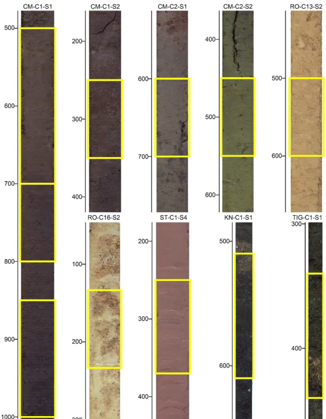
Cores were obtained from floodplain sites in the upper Severn, Wye and lower Boyne catchments and target elements were Si, K, Ti, Rb and Zr for the Holocene flooding study (Table 1 and Figure 1). The Zr/Rb ratio (Dypvik and Harris, 2001;Chen et al., 2006; Kylander et al., 2011) has previously been used as a grain size proxy in the upper Severn to produce a Late Holocene flood chronology (Jones et al., 2012). Si, K and Ti can potentially form alternative grain size proxy ratios (e.g. Oldfield et al., 2003; Chawchai et al., 2016). Cores were collected from the Avoca catchment and target elements were Pb, Cu and Zn for the contamination study. The core sections used for testing were selected as representative of the range of grain sizes, organic contents and sediment source areas present in the cores in the two studies. Test sections were limited to 100-200 mm in length to reduce the time required for multiple XRF scans of each section.
Figure 1. Test sections in cores from the flooding study and the contamination study. The scale for each core gives the depth in mm below the top of the individual section (including the casing), rather than the total depth below the ground surface.
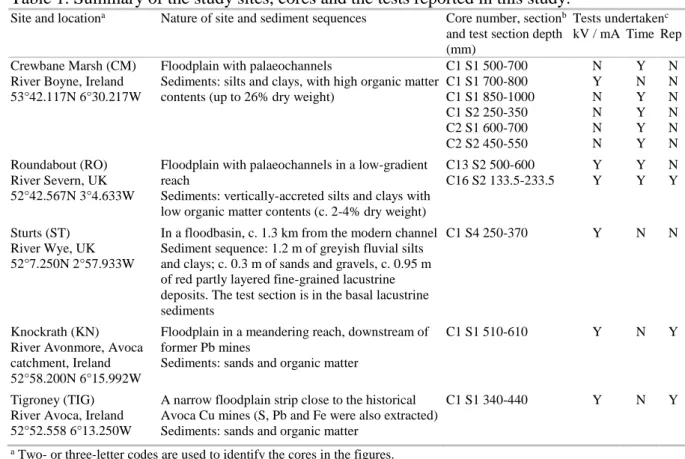
Table 1. Summary of the study sites, cores and the tests reported in this study.
Site and locationa Nature of site and sediment sequences Core number, sectionb
and test section depth (mm)
Tests undertakenc
kV / mA Time Rep Crewbane Marsh (CM)
River Boyne, Ireland 53°42.117N 6°30.217W
Floodplain with palaeochannels
Sediments: silts and clays, with high organic matter contents (up to 26% dry weight)
C1 S1 500-700 C1 S1 700-800 C1 S1 850-1000 C1 S2 250-350 C2 S1 600-700 C2 S2 450-550 N Y N N N N Y N Y Y Y Y N N N N N N Roundabout (RO) River Severn, UK 52°42.567N 3°4.633W
Floodplain with palaeochannels in a low-gradient reach
Sediments: vertically-accreted silts and clays with low organic matter contents (c. 2-4% dry weight)
C13 S2 500-600 C16 S2 133.5-233.5 Y Y Y Y N Y Sturts (ST) River Wye, UK 52°7.250N 2°57.933W
In a floodbasin, c. 1.3 km from the modern channel Sediment sequence: 1.2 m of greyish fluvial silts and clays; c. 0.3 m of sands and gravels, c. 0.95 m of red partly layered fine-grained lacustrine deposits. The test section is in the basal lacustrine sediments
C1 S4 250-370 Y N N
Knockrath (KN) River Avonmore, Avoca catchment, Ireland 52°58.200N 6°15.992W
Floodplain in a meandering reach, downstream of former Pb mines
Sediments: sands and organic matter
C1 S1 510-610 Y N Y
Tigroney (TIG) River Avoca, Ireland 52°52.558 6°13.250W
A narrow floodplain strip close to the historical Avoca Cu mines (S, Pb and Fe were also extracted) Sediments: sands and organic matter
C1 S1 340-440 Y N Y
a Two- or three-letter codes are used to identify the cores in the figures. b C = core, S = section.
c kV / mA – tests varying tube voltage and current; Time – tests varying XRF exposure time; Rep – repeatability of scanning
results
Cores for the flooding study were collected in metre sections in 50 mm diameter plastic tubes using a handheld percussion corer. Cores for the contamination study were collected with a hand auger and subsampled using 18 mm wide plastic u-channels in metre lengths.
XRF core scans were performed using the Itrax instrument at University College Dublin, which has a 100 m beam width, with a Mo anode X-ray tube. Samples were covered with 1.5 μm thick polyethylene film during scanning. Tests of the effects of varying tube voltage, current and exposure time on SNRs and of measurement repeatability were carried out on the sections shown in Table 1 and Figure 1. Scanning intervals were 500 m for cores in the flooding study and 1 mm for the contamination study.
SNRs were calculated for each target element in each XRF spectrum using the method of Ernst et al. (2014), which does not attempt to account for overlaps between peaks. In this method, the signal (S) is calculated as the total counts in detector channels within the peak range (TC) minus the XRF background (BG).
𝑆 = 𝑇𝐶 − 𝐵𝐺 (1)
The XRF background is the mean of the mean pre-peak counts per channel (PP1) and mean post-peak counts per channel (PP2) multiplied by the number of channels within the peak range (C).
𝐵𝐺 = 𝐶 × (𝑃𝑃1+𝑃𝑃2
2 ) (2)
The noise (N) is the square root of the XRF background:
𝑁 = √𝐵𝐺 (3)
Further explanation and a worked example are given by Ernst et al. (2014). This method was originally developed for XRF spectra from glass fragments, characterized by near-linear increases in background from low to high energies. Wet sediment produces spectra with a higher, non-linear background which increases to a maximum and then declines, potentially resulting in an over- or underestimation of SNRs. With the exception of the Zr peak, as a result of its proximity to the incoherent scatter peak, the effect is likely to be relatively minor because the curvature of the background beneath individual element peaks is low.
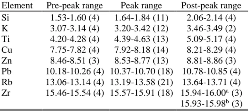
The channels (the energy range in keV) used for each element peak and for the pre-peak and post-peak background were determined by inspection of the sum of spectra for all test scans (Table 2). For Zr, two post-peak background ranges were identified, because of the change in shape of this peak with increasing tube voltage. A program created with Perl was used to calculate SNRs for each target element for all spectra in each test section. For each target element, the program extracted the counts in the relevant detector channels from the text files
recorded for each spectrum, performed the calculations and wrote the results for each calculated variable to a single output file for all spectra in the test section. Percentiles of the SNR distribution were calculated for each element within each test section.
Five combinations of tube voltage and current were tested initially: 30 kV 30 mA, 30 kV 50 mA, 40 kV 30 mA, 40 kV 40 mA and 50 kV 30 mA. 40 kV 35 mA was later added to this list because the 40 kV 40 mA combination appeared likely to result in detector saturation for some samples. Tests on the Crewbane Marsh, the Sturts, Knockrath and Tigroney cores also included 30kV 40 mA.
Table 2. Energy ranges in keV and number of channels (in brackets) used to calculate signal-to-noise ratios.
Element Pre-peak range Peak range Post-peak range Si 1.53-1.60 (4) 1.64-1.84 (11) 2.06-2.14 (4) K 3.07-3.14 (4) 3.20-3.42 (12) 3.46-3.49 (2) Ti 4.20-4.28 (4) 4.39-4.63 (13) 5.09-5.17 (4) Cu 7.75-7.82 (4) 7.92-8.18 (14) 8.21-8.29 (4) Zn 8.46-8.51 (3) 8.53-8.77 (13) 8.81-8.86 (3) Pb 10.18-10.26 (4) 10.37-10.70 (18) 10.78-10.85 (4) Rb 13.06-13.14 (4) 13.19-13.58 (21) 13.64-13.71 (4) Zr 15.46-15.54 (4) 15.57-15.91 (18) 15.94-16.00a(3) 15.93-15.98b(3) a for scans at 30 kV tube voltage.
b for scans at 40 kV or 50 kV tube voltage.
Exposure times of 10, 15, 20, 30, 60 and 120 seconds were tested in the flooding study, resulting in measurement times for a 100 mm section and a 500 m step size of c. 0.6, 0.9, 1.2, 1.7, 3.4 and 6.7 hours. The variable scan times resulted in substantial differences in the degree of heating of the samples and the likelihood of progressive desiccation during the series of test scans. Results are plotted as the increase in median SNR with increasing exposure time for each test section, and each combination of tube voltage and current used (Figure 4). Tests of exposure time were not undertaken for the contamination study.
Repeatability of XRF scan results was assessed using a set of nine successive scans. The Roundabout Core 16 test section was scanned at 40 kV 35 mA for 30 seconds and two repeatability tests were conducted on the Knockrath and Tigroney test sections at 30 kV 50 mA 5 s and at 50 kV 30 mA 5 s. Results are given for both signal calculations on the raw spectra and the modelled peak areas calculated by the Q-Spec program. Results for the Roundabout Core 16 test section were post-processed using Q-Spec, with a maximum of ten iterations for model fitting. Modelled peak areas for the spectrum at 158.5 mm depth in test scan 8 were excluded from calculation of the mean and standard deviation (Figure 5) because of a poor fit to the recorded spectrum (MSE>100). The standard deviation was calculated for each measurement and the mean standard deviation was calculated for the whole test section (cf. International Organization for Standardization, 1994).
3. Signal-to-noise ratios
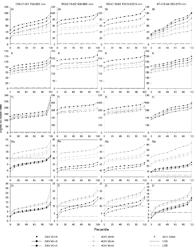
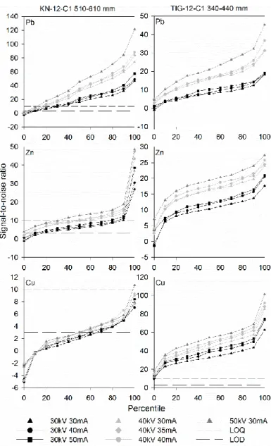
SNRs were greatest for Ti (>100) and K (>57) and least for Zr (<29) and Rb (<64) in the flooding study (Figure 2). As tube voltage was increased from 30 kV to 50 kV, median SNRs were multiplied by factors of 0.57 (Si), 0.85 (K), 0.98 (Ti), 3.05 (Rb) and 1.85 (Zr) (Table 3). An increase in the background level and a decrease in peak area produced the decrease in SNRs for the lighter elements. Increasing tube current from 30 mA to 50 mA increased median SNRs by factors of 1.26 (Si), 1.21 (K), 1.21 (Ti), 1.25 (Rb) and 1.24 (Zr). SNRs ranged from 0 to a maximum of 101 for Cu, 49 for Zn and 121 for Pb (Figure 3). Median SNRs increased by factors of 1.57 (Cu), 2.01 (Zn) and 2.78 (Pb) as tube voltage was increased from 30 kV to 50 kV. Increasing tube current from 30 mA to 50 mA increased median SNRs by factors of 1.18 (Cu), 1.21 (Zn) and 1.33 (Pb). The increase in median SNRs with increased tube voltage rises with increasing energy of the peak measured for an element, with the exception of Zr. The change in SNRs with an increase in tube current from 30 mA to
50 mA is similar for the seven target elements measured using their K peaks, but for Pb, measured using its L peak, it is noticeably larger.
Table 3. Factors by which median signal-to-noise ratios are increased with increasing tube voltage and tube current. The standard deviation is given in brackets beneath each factor.
Voltage Flood chronologies a Floodplain contamination c
increased from Si K Ti Rb Zr Cu Zn Pb 30 kV to 40 kV 0.750 (0.071) 0.938 (0.021) 1.020 (0.029) 2.096 (0.092) 1.657 (0.055) 1.320 (0.007) 1.605 (0.051) 2.013 (0.082) 40 kV to 50 kV 0.752 (0.044) 0.908 (0.020) 0.965 (0.033) 1.455 (0.041) 1.114 (0.041) 1.192 (0.101) 1.253 (0.080) 1.381 (0.062)
Current Flood chronologies b Floodplain contamination c
increased from Si K Ti Rb Zr Cu Zn Pb 30 mA to 40 mA 1.209 (0.064) 1.121 (0.023) 1.121 (0.005) 1.140 (0.022) 1.073 (0.044) 1.187 (0.003) 1.119 (0.028) 1.136 (0.043) 40 mA to 50 mA 1.108 (0.053) 1.096 (0.033) 1.099 (0.013) 1.066 (0.016) 1.134 (0.026) 0.996 (0.071) 1.085 (0.066) 1.171 (0.071)
a = Mean of sections CM C1 S1 700-800, RO C13 S2 500-600, RO C16 S2 133.5-233.5 and ST C1 S4 250-370. b = Mean of sections CM C1 S1 700-800 and ST C1 S4 250-370.
c = Mean of sections KN C1 S1 510-610 and TIG C1 S1 340-440
All SNRs for Si, K and Ti were greater than the LOQ. For the remaining elements the proportion of SNRs below both LOD and LOQ decreases with increasing tube voltage and current. Maximum percentages of measurements below the LOD and LOQ are 14.4% and 99.5% for Rb at Crewbane Marsh and 19.9% and 99.2% for Zr at the Sturts. 98% of Cu SNRs are below the LOQ in the Knockrath test section. Up to 89.1% of Zn SNRs at Knockrath and 74.6% for Pb in the Tigroney core are below the LOQ.
Figure 2. Change in SNRs with tube voltage and current for Si, K, Ti, Rb and Zr in XRF scans of test sections from the Crewbane Marsh (left column; CM C1 S1) , Roundabout (middle columns; RO C13 S2 and RO C16 S2) and Sturts (right column; ST C1 S4) sites performed at 500 µm resolution and 30 seconds exposure time. The distribution of values in the measurements for each test section in each scan is expressed as percentiles. Apparently negative SNRs occur where the ‘total counts’ for the peak are less than the ‘background’, resulting in a negative ‘signal’.
Figure 3. Change in SNRs with tube voltage and current for Cu, Zn and Pb in XRF scans of test sections from the Knockrath and Tigroney sites performed at 1 mm resolution. Apparently negative SNRs occur where the ‘total counts’ for the peak are less than the ‘background’, resulting in a negative ‘signal’.
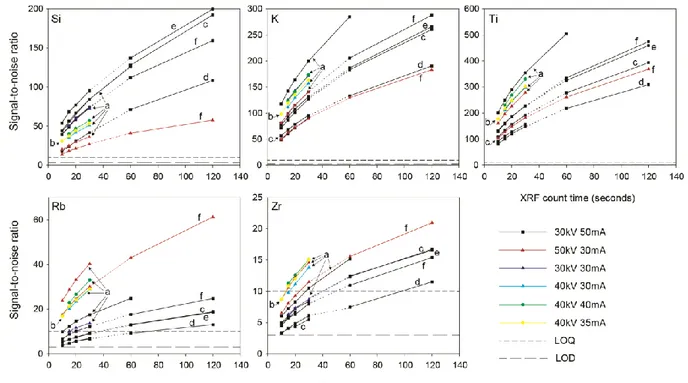
For K, Ti, Rb and Zr median SNR is increased by a factor of 1.23 at 15 seconds, 1.42 at 20 seconds and 1.74 at 30 seconds, 2.48 at 60 seconds and 3.50 at 120 seconds relative to the SNR for a 10 second exposure time for all combinations of tube voltage and current (Figure 4 and Table 4), in line with expected increases in SNRs proportional to the square root of the exposure time (Ernst et al. 2014). SNRs for Si increase by factors of 1.27 (15 seconds), 1.51
(20 seconds), 1.91 (30 seconds), 2.88 (60 seconds) and 4.23 (120 seconds), relative to the median for a 10 second exposure time.
Table 4. Factors by which median signal-to-noise ratios are increased with increasing exposure time. The standard deviation is given in brackets beneath each factor.
Exposure time increased from Si K Ti Rb Zr 10 to 15 secondsa 1.270c (0.038) 1.223c (0.018) 1.229c (0.011) 1.233c (0.042) 1.225c (0.032) 10 to 20 secondsa 1.515c (0.081) 1.415c (0.030) 1.427c (0.028) 1.442c (0.050) 1.397c (0.039) 10 to 30 secondsa 1.910c (0.173) 1.740c (0.056) 1.748c (0.039) 1.744c (0.055) 1.729c (0.054) 10 to 60 secondsb 2.882d (0.521) 2.518d (0.114) 2.500d (0.092) 2.481d (0.057) 2.423d (0.105) 10 to 120 secondsb 4.232d (0.908) 3.570d (0.181) 3.542d (0.138) 3.531d (0.076) 3.376d (0.141)
a = Mean of sections CM C1 S1 500-700, CM C1 S1 850-1000, CM C1 S2 250-350, CM C2 S1 600-700, all
scanned at 30 kV 50 mA, CM C2 S2 450-550 and RO C13 S2 500-600, scanned at 30 kV 50 mA and at 50 kV 30 mA, and RO C16 S2 133.5-233.5, scanned at 40 kV 35 mA.
b = Mean of sections CM C1 S1 580-700, CM C1 S2 270-350, CM C2 S1 620-700 and CM C2 S2 500-550, the
latter scanned at both 30 kV 50 mA and 50 kV 30 mA.
Figure 4. Change in median SNRs with exposure time for Si, K, Ti, Rb and Zr in XRF scans of test sections from the Crewbane Marsh and Roundabout sites. The test section used for each analysis is indicated by lower case letters on the graphs: a, RO C13 S2; b, RO C16 S2; c, CM C1 S1; d, CM C1 S2; e, CM C2 S1; f, CM C2 S2. Shortened test sections were used in some cases for scans at 60 and 120 seconds. Dashed lines connect the results from scans of these shortened test sections to the results for the full test section measured at shorter
exposure times. Median SNRs of Rb and Zr below the LOQ indicate the unsuitability of the profiles for interpretation at the selected exposure time.
4. Repeatability of scan results
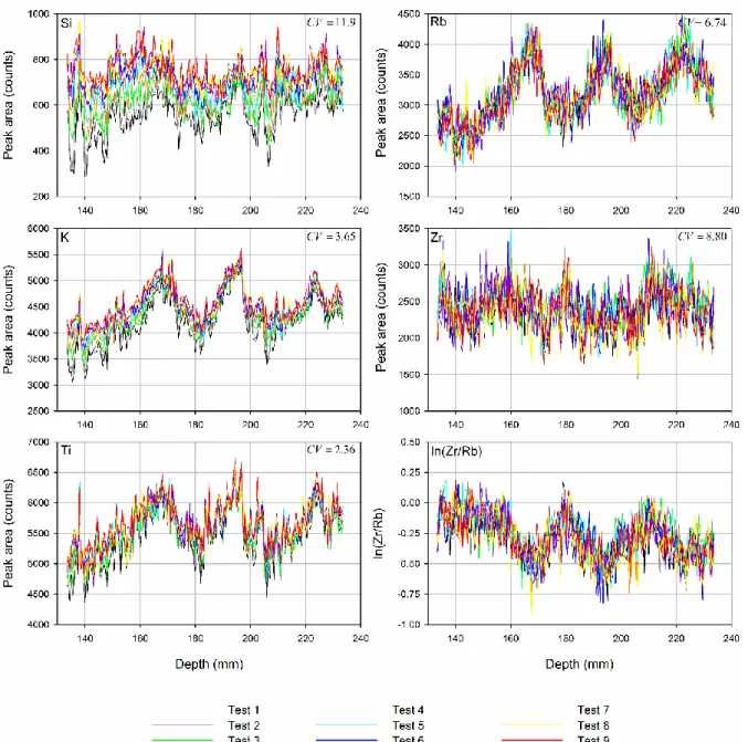
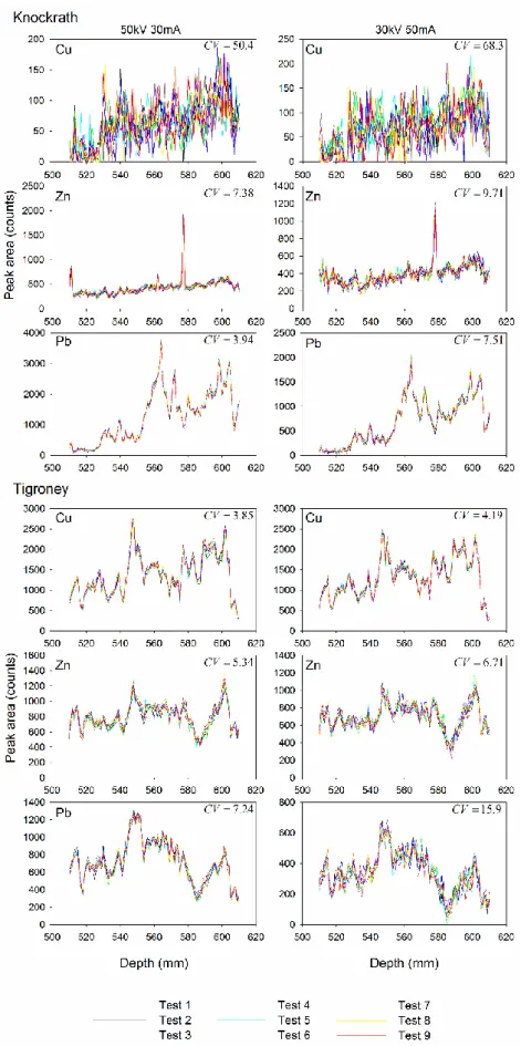
Profile shape is most consistently reproduced for Ti in the flooding study (Figure 5). Major peaks and troughs are consistently reproduced between scans for K, Rb and ln(Zr/Rb) and to a lesser extent Zr. For Si, X-ray fluorescence intensity increases progressively through the first six scans and similar patterns are also apparent for K and Ti. The greatest increases were observed for the lowest initial intensities. Profile shape is consistently reproduced in the repeat scans in the contamination study for Cu and Zn at Tigroney and for Pb at both sites, with the main features also consistently reproduced for Zn at Knockrath (Figure 6), but profile shape for Cu at Knockrath is dominated by noise.
Figure 5. Repeatability of scan measurements in the Core RO C16 S2 test section for Si, K, Ti, Rb, Zr and ln(Zr/Rb) at 40 kV 35 mA and 30 seconds. Test numbers indicate the order in which the scans were performed to demonstrate the effects of progressive changes in the sample on the results for Si, K and Ti. The mean coefficient of variation for the test section is given on the graph for each element.
Figure 6. Repeatability of scan measurements in the Knockrath and Tigroney test sections for Cu, Zn and Pb at 50 kV 30 mA and at 30 kV 50 mA. The mean coefficient of variation for the test section is given on each graph.
Si had the highest coefficient of variation for modelled results in the flooding study and Ti the lowest, followed by K, while values for Rb and Zr were moderate. Zr shows a substantial reduction in coefficient of variation from the signal calculation data (13.09%) to modelled peak intensities. For Cu the coefficient of variation is substantially higher at Knockrath than at Tigroney while for Pb and Zn the opposite is the case. Mean standard deviations were higher for modelled results (Ti 132.2, Rb 215.8, Zr 211.0) than for the signal calculations (Ti 121.4, Rb 187.2, Zr 190) for the flooding study. The model-fitting process is a source of variability in the modelled results. The modelling of non-linear background beneath element peaks and of overlaps between element peaks, which are not considered in the signal calculation method, may contribute to this effect. Mean standard deviations were greater for signal calculation data than for modelled results for the contamination study (e.g. 39 and 30 for Zn, 77.7 and 51.0 for Pb at Knockrath scanned at 50kV 30 mA). The short exposure time resulted in a high degree of variability between the counts in adjacent channels within the spectrum which is smoothed out by the model.
5. Discussion
The value of testing the effects of varying tube voltage, tube current and exposure time on SNRs of target element peaks is demonstrated by the differences between SNRs obtained using different instrument parameters. The results indicate the benefit of selecting instrument parameters for particular target elements especially where they are likely to be present at low concentrations. The choice of X-ray tube voltage is likely to have a greater impact than of tube current on data quality. Careful selection of these parameters for XRF core scans of any sediment type may produce significant improvements in SNRs without increasing the time taken for the scan. However, selecting optimal tube voltage and current may be difficult
where target elements have peaks across the range of energies measured in the XRF spectrum. For example, if Si and Zr are both target elements in a study in which each core can only be scanned once, tube voltage can be optimised for either one or the other of these elements or a tube voltage selected between these two optimal values. In each case, SNRs for one or both elements will be less than the maximum attainable within this range of tube voltage values. The varying proportions of measurements that fall below the LOD and LOQ show the value of examining measured XRF spectra when evaluating and interpreting the results of XRF core scans.
The method used by Ernst et al. (2014) provides a rapid means of assessing whether element concentrations are above or below the LOD and LOQ in a single spectrum, of evaluating the distribution of SNRs within a section and of comparing scan results for a range of Itrax micro-XRF parameters when scanning cores of lacustrine and marine sediments, as well as floodplain sediment cores as demonstrated in this study. These calculations can be automated using a simple computer program. The method for estimating background counts assumes a linear background (Ernst et al., 2014), but the background beneath the Zr peak at 40 kV and 50 kV is curved because it is close to the Mo incoherent scatter peak. The low SNRs for Zr at 30 kV are likely to be accurate while the higher SNRs for scans at 40 kV and 50 kV are underestimates. This reduced the apparent effect of increasing tube voltage on Zr. An estimate of the actual SNR values for Zr at 40 kV and 50 kV was obtained by substituting the modelled result for the calculated signal, and subtracting this value from the total counts to estimate the true background. This gives median SNRs for Crewbane Marsh, Roundabout Core 16 and the Sturts of 12.5, 19.2 and 10.5 at 40 kV and 19.9, 27.2 and 16.0 at 50 kV respectively. This gives an increase in median SNRs of a factor of 3.25 as tube voltage is increased from 30 kV to 50 kV, slightly higher than the factor calculated for Rb and
consistent with the increasing magnitude of factors for peaks towards the higher energy part of the spectrum.
The factors in Tables 3 and 4 can be used to estimate the change in SNRs that could be obtained by adjusting instrument parameters for floodplain cores, avoiding the need for a full set of instrument parameter tests for a new site for these target elements. These factors may potentially be applicable to other sediment types but, if not, could be estimated in the manner used in this study for marine and lacustrine samples, for example. The factors in Tables 3 and 4 were calculated using median SNRs but also provide a useful approximation of the changes that result from alteration of instrument parameters for the majority of the SNR distribution. The 10th percentile of the distribution, which avoids outliers at the tail of the SNR
distribution, could be used to determine whether particular values of tube voltage, current and exposure time are likely to deliver measurements above the LOQ for the majority of the element profile. Although Huang et al. (2016) concluded that increasing Itrax XRF exposure time gives insignificant improvements in accuracy, Figure 4 demonstrates that for elements such as Rb and Zr increasing exposure time can substantially increase the proportion of measurements with SNRs greater than the LOQ.
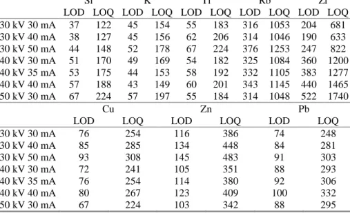
Suggested heuristics for assessing XRF core scan data quality use threshold values of counts for peak area that are the same for all elements considered (e.g. minimum 500 counts (Brown, 2015)). To compare the usefulness of such heuristics with the SNR method, regression of modelled results on SNRs was used to estimate the values of the LOD and LOQ for each combination of tube voltage and current (Table 5). The results show ranges of up to an order of magnitude in the values of LODs and LOQs of the different elements and of between 1.2 and 2.7 times the lowest value of the LOD and LOQ for the different combinations of tube
voltage and current for single elements in these floodplain sediments. These results suggest that heuristics based on a single threshold value are unsuitable for assessing data quality of an element profile. It is recommended that SNRs be routinely calculated for each target element in each XRF spectrum for all types of sediment to assess profile suitability for interpretation using the LOQ. Depending on sample composition and target elements this may require the use of more sophisticated methods of calculation, which account for peak overlap and non-linear background, to produce accurate results. The values in Table 5 also suggest that an evaluation of the quality of XRF core scan data in some previously published studies may find unexpectedly low SNRs for some element profiles, or parts of profiles, that have been used to infer environmental change, particularly for trace elements. If an assessment of SNRs were conducted in such cases, it may be found that some inferences drawn from the data were less well supported than previously thought or, if based on a single element profile, were not supported at all.
Table 5. Limits of detection (LOD) and quantification (LOQ) in counts for each combination of tube voltage and current estimated in floodplain sediments using regression of modelled results on signal-to-noise ratios. Linear regression was used for each element except K, for which a second order polynomial provided a better fit to the data. Exposure times were 30 seconds for the flooding study and 5 seconds for the floodplain contamination study.
Si K Ti Rb Zr
LOD LOQ LOD LOQ LOD LOQ LOD LOQ LOD LOQ 30 kV 30 mA 37 122 45 154 55 183 316 1053 204 681 30 kV 40 mA 38 127 45 156 62 206 314 1046 190 633 30 kV 50 mA 44 148 52 178 67 224 376 1253 247 822 40 kV 30 mA 51 170 49 169 54 182 325 1084 360 1200 40 kV 35 mA 53 175 44 153 58 192 332 1105 383 1277 40 kV 40 mA 57 188 43 149 60 201 343 1145 440 1465 50 kV 30 mA 67 224 57 197 55 184 314 1048 522 1740 Cu Zn Pb
LOD LOQ LOD LOQ LOD LOQ
30 kV 30 mA 76 254 116 386 74 248 30 kV 40 mA 85 285 134 448 84 281 30 kV 50 mA 93 308 145 483 91 303 40 kV 30 mA 72 241 105 351 88 293 40 kV 35 mA 76 254 114 380 92 306 40 kV 40 mA 80 267 123 409 100 332 50 kV 30 mA 67 224 103 342 88 295
The increase in Si, K and Ti intensities in successive scans of the Roundabout Core 16 test section suggests that the sample moisture content may be progressively reduced during the set of scans as a result of sample heating, in spite of the film covering the sediment surface, although it is possible that changes to other components within the sediment are responsible for the increase in element intensities. Fluorescence emitted by the lighter elements, including Si and K, and also Ti, is absorbed by water within the sediment, reducing element intensities in the XRF spectrum (Tjallingii et al., 2007; Wilhelms-Dick et al., 2012; MacLachlan et al., 2015). The reduction in the intensity of the fluorescence from these elements as a result of absorption by interstitial water is dependent on sediment water content (Kido et al., 2006). The cause of this increase in fluorescence intensity of the lighter elements requires further investigation and, if it is confirmed to be the result of changing water content, a correction for varying moisture content may be required in these cores (see for example Boyle et al., 2015).
For the elements with the highest SNRs in these floodplain sediments, coefficients of variation are below 5% for a 30 second exposure time, as reported by Jarvis et al. (2015) in their study. In the test sections with the highest concentrations of contaminant Pb or Cu in the Avoca catchment, coefficients of variation below 5% are attained with an exposure time of only 5 seconds. The confidence with which profile shape can be interpreted depends not only on the coefficient of variation but also upon the range of values, rather than the mean value, within the profile. The nature of the profile shape changes that can be interpreted is also affected by these factors: repeat scans of Zr indicate that sustained changes in element intensity, both gradual and abrupt, are consistently replicated between scans while rapidly reversed changes of similar magnitude are not (compare the profile below 200 mm with the section around 185 mm depth for test 9 in Figure 5). Repeat measurements of ln(Zr/Rb) in the test section indicate that the centimetre-scale changes in this ratio constitute a signal but the
millimetre-scale changes appear to be noise, which may affect interpretation of grain size proxy ratios for producing flood records.
The tests of tube voltage, tube current, exposure time and repeatability reported above have supported identification of the cores in which ln(Zr/Rb) and other geochemical grain size proxies can be used, of which grain size proxy is most suitable in each case and of instrument parameters that will provide good data quality in the flooding study. In the floodplain contamination study, these tests have demonstrated the potential for using the Itrax instrument, with the optimised tube voltage and current, for rapid assessment of downcore variations in contaminant metal concentrations in historically mined catchments. While the values given in Tables 3, 4 and 5 may not necessarily be applicable to sediment from all environments, the methods used in this study could be applied to produce comparable sets of values for lacustrine, marine and other types of sediment analysed using the Itrax core scanner.
6. Conclusion
SNRs estimated from XRF core scan spectra, and the LOQ, provide an objective method for both assessing instrument parameter suitability for meeting investigation objectives and establishing element profile suitability for reconstructing environmental changes. Selecting instrument parameters, notably X-ray tube voltage, for specific target elements can produce a substantial improvement in SNRs of these element peaks. SNRs should be used in preference to heuristics based on a value of counts for assessing whether scan results can be meaningfully interpreted. Element level variations within the majority of test sections are substantially greater than the variability in the results for individual measurements.
Acknowledgements
We are grateful to landowners and farmers in the Severn, Wye, Boyne and Avoca valleys for allowing us to take cores on their land. We also thank Ciara Fleming and David Colgan for assistance in the field. We wish to thank Eamonn Hynes for writing the program used to calculate signal-to-noise ratios.
Funding
This work was supported by a Marie Curie Actions Intra-European Fellowship (project number 300623). The Itrax XRF core scanner at University College Dublin was funded by a HEA Equipment Renewal Grant.
Declarations of interest: none
References
Boyle, J.F., Chiverrell, R.C., Schillereff, D., 2015. Approaches to water content correction and calibration for μXRF core scanning: comparing X-ray scattering with simple regression of elemental concentrations. In: Croudace, I.W., Rothwell, R.G. (Eds.) Micro-XRF Studies of Sediment Cores. Springer, Dordrecht, pp. 373-390.
Brown, E.T., 2015. Estimation of biogenic silica concentrations using scanning XRF: Insights from studies of Lake Malawi sediments. In: Croudace, I.W., Rothwell, R.G. (Eds.) Micro-XRF Studies of Sediment Cores. Springer, Dordrecht, pp. 267-277.
Chawchai, S., Kylander, M.E., Chabangborn, A., Löwemark, L., Wohlfarth, B., 2016. Testing commonly used X-ray fluorescence core scanning-based proxies for organic-rich lake sediments and peat. Boreas 45, 180-189.
Chen, J., Chen, Y., Liu, L., Ji, J., Balsam, W., Sun, Y., Lu, H., 2006. Zr/Rb ratio in the Chinese loess sequences and its implication for changes in the East Asian winter monsoon strength. Geochimica et Cosmochimica Acta 70, 1471-1482.
Dypvik, H., Harris, N.B., 2001. Geochemical facies analysis of fine-grained siliciclastics using Th/U, Zr/Rb and (Zr+Rb)/Sr ratios. Chemical Geology 181, 131-146.
Ernst, T., Berman, T., Buscaglia, J., Eckert-Lumsdon, T., Hanlon, C., Olsson, K., Palenik, C., Ryland, S., Trejos, T., Valadez, M., Almirall, J.R., 2014. Signal-to-noise ratios in forensic glass analysis by micro X-ray fluorescence spectrometry. X-ray Spectrometry 43, 13-21.
Huang, J.-J., Löwemark, L., Chang, Q., Lin, T.-Y., Chen, H.-F., Song, S.-R., Wei, K.-Y., 2016. Choosing optimal exposure times for XRF core-scanning: Suggestions based on the analysis of geological reference materials. Geochemistry, Geophysics, Geosystems 17, 1558-1566.
International Organization for Standardization, 1994. ISO 5725-2 Accuracy (trueness and precision) of measurement methods and results - Part 2: Basic method for the determination
Jarvis, S., Croudace, I.W., Rothwell, R.G., 2015. Parameter optimisation for the ITRAX core scanner. In: Croudace, I.W., Rothwell, R.G. (Eds.) Micro-XRF Studies of Sediment Cores. Springer, Dordrecht, pp. 535-562.
Jones, A.F., Macklin, M.G., Brewer, P.A., 2012. A geochemical record of flooding on the upper River Severn, UK, during the last 3750 years. Geomorphology 179, 89-105.
Kido, Y., Koshikawa, T., Tada, R., 2006. Rapid and quantitative major element analysis method for wet fine-grained sediments using an XRF microscanner. Marine Geology 229, 209-225.
Kylander, M.E., Ampel, L., Wohlfarth, B., Veres, D., 2011. High-resolution X-ray fluorescence core scanning analysis of Les Echets (France) sedimentary sequence: new insights from chemical proxies. Journal of Quaternary Science 26, 109-117.
MacLachlan, S.E., Hunt, J.E., Croudace, I.W., 2015. An empirical assessment of variable water content and grain-size on X-ray fluorescence core-scanning measurements of deep sea sediments. In: Croudace, I.W., Rothwell, R.G. (Eds.) Micro-XRF Studies of Sediment Cores. Springer, Dordrecht, pp. 173-185.
Oldfield, F., Wake, R., Boyle, J., Jones, R., Nolan, S., Gibbs, Z., Appleby, P., Fisher, E., Wolff, G., 2003. The late-Holocene history of Gormire Lake (NE England) and its catchment: a multiproxy reconstruction of past human impact. The Holocene 13, 677-690.
fluorescence core- scanning measurements in soft marine sediments. Geochemistry, Geophysics, Geosystems 8, Q02004.
Wilhelms-Dick, D., Westerhold, T., Röhl, U., Wilhelms, F., Vogt, C., Hanebuth, T.J.J., Römmermann, H., Kriews, M., Kasten, S., 2012. A comparison of mm scale resolution techniques for element analysis in sediment cores. Journal of Analytical Atomic Spectrometry 27, 1574-1584.