Library of model components for process simulation relevant to production activities, Prototype 1 versions.

(1)

HAL Id: hal-02818052

https://hal.inrae.fr/hal-02818052

Submitted on 6 Jun 2020

HAL is a multi-disciplinary open access archive for the deposit and dissemination of sci-entific research documents, whether they are pub-lished or not. The documents may come from teaching and research institutions in France or abroad, or from public or private research centers.

L’archive ouverte pluridisciplinaire HAL, est destinée au dépôt et à la diffusion de documents scientifiques de niveau recherche, publiés ou non, émanant des établissements d’enseignement et de recherche français ou étrangers, des laboratoires publics ou privés.

Trevisan

To cite this version:

M. Donatelli, A.E. Rizzoli, F.K. van Evert, B. Rutgers, Christian Dupraz, et al.. Library of model components for process simulation relevant to production activities, Prototype 1 versions.. [Technical Report] 27, 2007. �hal-02818052�

(2)

System for Environmental and Agricultural Modelling;

Linking European Science and Society

Report no.: 27 June 2007 Ref: D3.2.18

ISBN no.: 90-8585-115-7 and 978-90-8585-115-8

Library of model components for process simulation

relevant to production activities, Prototype 1

versions

Donatelli, M, Rizzoli, A.E., van Evert, F.K., Rutgers, B., Trevisan, M.

et al.

(3)

SEAMLESS integrated project aims at developing an integrated framework that allows ex-ante assessment of agricultural and environmental policies and technological innovations. The framework will have multi-scale capabilities ranging from field and farm to the EU25 and globe; it will be generic, modular and open and using state-of-the art software. The project is carried out by a consortium of 30 partners, led by Wageningen University (NL). Email: seamless.office@wur.nl

Internet: www.seamless-ip.org

Authors of this report and contact details

Name: Marcello Donatelli Partner acronym: CRA-ISCI

Address: Via di Corticella, 133 – 40128 Bologna, Italy E-mail:m.donatelli@isci.it

Name: Andrea Rizzoli Partner acronym: IDSIA

Address: Manno-Lugano, Switzerland E-mail: andrea@idsia.ch

Name: Frits van Evert, Ben Rutgers Partner acronym: PRI

Address: Wageningen, The Netherlands E-mail:frits.vanevert@wur.nl

For the AgroManagement component:

Name: Marcello Donatelli Partner acronym: CRA-ISCI

Address: Via di Corticella, 133 – 40128 Bologna, Italy E-mail: m.donatelli@isci.it

For the AgroChemicals component:

Name: Marco Trevisan, Andrea Sorce, Matteo Balderacchi, Andrea Di Guardo

Partner acronym: CRA-UNICATT Address: Piacenza, Italy

E-mail: marco.trevisan@unicatt.it

For the Crop component:

Name: Frank Ewert, Peter Leffelaar, Eelco Meuter, Myriam Adam

Partner acronym: WUR-PPS Address: Wageningen, The Netherlands

E-mail: frank.ewert@wur.nl

For the Soil Carbon and Nitrogen component:

Name: Jo Smith, Pia Gottschalk Partner acronym: UNIABDN

Address: Aberdeen, UK E-mail:jo.smith@abdn.ac.uk

For the Soil Water and Runoff components:

Name: Marco Acutis, Patrizia Trevisiol, Antonella Gentile

Partner acronym: CRA-UNIMI Address: Milano, Italy

E-mail: marco.acutis@unimi.it

For the Weather components:

Name: Marcello Donatelli, Gianni Bellocchi, Laura Carlini

Address: Bologna, Italy Partner acronym: CRA-ISCI

(4)

For the Grasses component:

Name: Michel Duru, Pablo Cruz, Myriam Adam Partner acronym: INRA Address: Toulouse, France

E-mail: michel.duru@toulouse.inra.fr

For the Vineyards/Orchards components:

Name: Christian Gary, Kamal Kansou, Jacques Wery Partner acronym: INRA Address: Montpellier, France

E-mail: christian.gary@cirad.fr

For the Agroforestry component:

Name: Christian Dupraz, Kamal Kansou Partner acronym: INRA

Address: Toulouse, France E-mail: dupraz@ensam.inra.fr

For theSoil Water 2 component:

Name: Erik Braudeau Partner acronym: CIHEAM-IRD

Address: Montpellier, France E-mail: erik.braudeau@ird.fr

Name: Pierre Martin Partner acronym: CIHEAM-CIRAD

Address: Montpellier, France E-mail: pierre.martin@cirad.fr

Disclaimer 1:

“This publication has been funded under the SEAMLESS integrated project, EU 6th Framework Programme for Research, Technological Development and Demonstration, Priority 1.1.6.3. Global Change and Ecosystems (European Commission, DG Research, contract no. 010036-2). Its content does not represent the official position of the European Commission and is entirely under the responsibility of the authors.”

"The information in this document is provided as is and no guarantee or warranty is given that the information is fit for any particular purpose. The user thereof uses the information at its sole risk and liability."

Disclaimer 2:

Within the SEAMLESS project many reports are published. Some of these reports are intended for public use, others are confidential and intended for use within the SEAMLESS consortium only. As a consequence references in the public reports may refer to internal project deliverables that cannot be made public outside the consortium.

When citing this SEAMLESS report, please do so as:

Donatelli, M, Rizzoli, A.E., van Evert, F.K., Rutgers, B., Trevisan, M. et al. 2007. Library of model components for process simulation relevant to production activities, Prototype 1 versions, SEAMLESS Report No.27, SEAMLESS integrated project, EU 6th Framework Programme, contract no. 010036-2, www.SEAMLESS-IP.org, 47 pp., ISBN no. 90-8585-115-7 and 978-90-8585-115-8.

(5)

(6)

General part

Objective within the project

Provide a library of discrete software units implementing models / utilities for use both by third parties and to build the Agricultural Production and Externalities Simulator (APES)

General Information

Task(s) and Activity code(s): T3.2 – A3.2.9

Input from (Task and Activity codes): T3.2 – A3.2.1/2/3/5/7

Output to (Task and Activity codes): T3.2 - A3.2.1/2/3/5/7/9 – WP5

Related milestones: M3.2.1

Executive summary

In systems analysis, it is common to deal with the complexity of an entire system by considering it to consist of interrelated sub-systems. This leads naturally to consider models as consisting of sub-models. Such a (conceptual) model can be implemented as a computer model that consists of a number of connected component models. Component-oriented designs actually represent a natural choice for building scalable, robust, large-scale applications, and to maximize the ease of maintenance in a variety of domains, including agro-ecological modelling.

The modular approach was chosen to develop Agricultural Production and Externalities Simulator (APES). APES is a modular simulation system targeted at estimating the biophysical behaviour of agricultural production systems in response to the interaction of weather, soils and different options of agro-technical management. Although a specific, limited set of components is available in the first release, the system is being built to incorporate, at a later time, other modules which might be needed to simulate processes not included in the first version. The processes are simulated in APES with deterministic approaches which are mostly based on mechanistic representations of biophysical processes. The criteria for selecting modelling approaches are based on the need for: 1) accounting for specific processes to simulate soil-land use interactions, 2) input data to run simulations, which may be a constraint at EU scale, 3) simulation of agricultural production activities of interest (e.g. crops, grasses, orchards, agroforestry), and 4) simulation of agro-management implementation and its impact on the system.

This report presents the current state of development of the model components being developed for APES and for third parties use. The intended use and modelling capabilities of each component are summarized.

(9)

Scientific and societal relevance

Creating a library of model components is a key part of developing a flexible simulation system that can be extended according to operational needs, and of sharing knowledge making available the relevant models for operational use. The modelling solutions and the implementation technology used are a realization of a goal being shared in the scientific community for more than a decade.

The envisioned impact is both on improving the use of resources by providing a way to avoid duplications, and by making available building blocks for quicker tool development, in order to match the demand from institutions and extension services.

(10)

Specific part

1 Introduction

In systems analysis, it is common to deal with the complexity of an entire system by considering it to consist of interrelated sub-systems. This leads naturally to think of models as made of sub-models. Such a (conceptual) model can be implemented as a computer model composed of a number of connected component models. An implementation based on component models has at least two major advantages. First, new models can be constructed by connecting existing component models of known and guaranteed quality together with new component models. This has the potential to increase the speed of development. Secondly, the predictive capabilities of two different component models can be compared, as opposed to compare whole simulation systems as the only option. Further, common and frequently used functionalities, such as numerical integration services, visualisation and statistical ex-post analyses tools, can be implemented as generic tools and developed once for all and easily shared by model developers.

As a consequence of the above, in the last decade there has been an increasing demand for modularity and replaceability in biophysical model development (e.g. Jones et al., 2001; David et al., 2002; Donatelli et al., 2003, 2004), aiming both at improving the efficiency of use of resources and at fostering higher quality of modelling units via specialization of model builders in a specific domain. The modular approach developed in the software industry is based on the concept of encapsulating the solution of a modelling problem in a discrete, replaceable, and interchangeable software unit. Such discrete units are called components. A software component can be defined as “a unit of composition with contractually specified interfaces and explicit context dependencies only. A software component can be deployed independently and is subject by composition by third parties” (Szypersky et al., 2002). Component-oriented designs actually represent a natural choice for building scalable, robust, large-scale applications, and to maximize the ease of maintenance in a variety of domains, including agro-ecological modelling (Argent, 2004). The concept of developing modular systems for biophysical simulation has lead to the development of several modelling frameworks (e.g. Simile, ModCom, IMA, TIME, OpenMI, SME, OMS, as listed in Argent and Rizzoli, 2004, and Rizzoli et al., 2004), which allow making use of components by linking them either together or to a simulation engine. In fact, three major parts of the implementation of models are usually prototype specific, resource intensive, and prevent transferability: (1) data input/output procedures (e.g. input/output data handling, file management), (2) common services (e.g. state variables integrator, simulation events handler) and (3) graphical user interfaces (GUI). Modelling frameworks can play a key role to address these issues. First, the framework allows segregating the application-specific parts of simulations from the code employed to accomplish common tasks, thus greatly enhancing code reuse (Hillyer et al., 2003). Second, by defining the elements of the framework that actually contain the model implementation and how those elements are used, a designer can be presented with a clear path from conceptual model to simulation (Hillyer et al., 2003). Furthermore, avoiding the reimplementation of common services allows the concentration of resources on the development of simulation components.

Developing a simulation system adopting the component-oriented paradigm poses specific challenges, both in terms of 1) biophysical model linking, and 2) implementation architecture.

(11)

About the former, the component-based architecture demands for defining and implementing sub-systems which minimize the need for links to other components, minimizing also the need for repeated communication across components. Even when a system to be simulated is divided into sub-systems which minimize the need of communication across them, data exchange prior to integration within a time step is needed, hence requiring an articulated interfaced which allows for such calls. Another conceptual problem, often attributed to component-based systems as intrinsically and potentially prone to mix and match “everything”, is shifted to components themselves using semantically rich interfaces which ensure that the linked variables are the correct ones. To illustrate the concept, if a component makes available a variable characterized by units, range of use, type and description, and another component requires the same variable as an input, the link can be considered correct if a check of the variable attributes can be successfully performed, whereas the correctness of using the variable as an input must be investigated within the component itself. The principle of applying “parsimony” is of course still valid in model building. For instance, there is no point in coupling two components in which the possible strong assumptions (and thus the limitations) of the former impose an unnecessary burden on the possibly extensive modelling capabilities of the latter; this, however, is a concept that applies both to monolithic and component based systems development. As always, it is the goal of both model application and system analysis which must suggest model choices, and this is independent of the type of implementation.

With regards to implementation architecture and use of modelling frameworks, there are two major problems: 1) the framework design and implementation must be optimized to balance carefully its flexibility and its usability to avoid incurring either a performance penalty or users having too steep a learning curve, and 2) developing components for a specific framework constrains their use to that framework.

In essence, two main options are available to overcome such problems. The most immediate is developing inherently reusable components (i.e. non framework specific), which can be used in a specific modelling framework by encapsulating them using dedicated classes called “wrappers”; such classes act as bridges between the framework and the component interface. The disadvantage of this solution is the creation of another “layer” in the implementation, which adds to the already implemented machinery in the framework. The appropriateness of this solution, both as ease of implementation and overall performance, must be evaluated case by case. The first prototypes of components developed in SEAMLESS for use in APES are based on this option, that is, developing non framework specific components which can be linked to different modelling frameworks, among which Modcom (Hillyer et al., 2003) is the one used in the current pre-release of APES. Other components under development, not available yet as discrete software units, are implemented as Modcom classes.

Regardless of the choice of developing framework specific or intrinsically reusable components, there is a basic choice which must be carefully evaluated prior to that and which is related, in general terms, to the framework as a flexible modelling environment to build complex models (model linking), but also to the framework as an efficient engine for simulation, calibration and simulation of model components (model execution).

Modern software technologies allow building flexible, coherent and elegant constructs, but that comes at a performance cost. Without even introducing Object Oriented Programming (OOP) and the meaning of the features cited later in this sentence, which is definitely beyond the scope of this report, it seems important to point out that the use of object-oriented programming constructs, which actually enhance flexibility, modularity and reuse of software, all nice things, require the compiler to use virtual methods calls, dynamic dispatching, and so on. All these operations are resource intensive and in some cases, they can heavily affect the code performance, and this becomes evident in applications in which such use is done thousand times every simulation step. Even if compiler technology and

(12)

implementation solutions are progressing rapidly to overcome the problems by enhancing dynamic code generation (e.g. Richter, 2005; Duffy, 2005; Golding, 2005; Pobar, 2005; Erisman 2006), the problem is not about re-designing or re-factoring software; instead, it is about the general strategy to follow. Be aware that we do not mean that such features should not be used, instead it addresses that using them at run-time is very costly. In other terms, the full use of OOP in the phase of building applications based on biophysical models is an extremely valuable resource, as it is to extend applications and to provide an effective architecture of applications themselves, but it probably should be minimized for use of biophysically based models at run-time. An alternative option is introduced in the next paragraph.

The second option to overcome the problems deriving from modelling framework architecture and use, as defined in the previous page, is far more interesting and can be very effective also with respect to other desirable features in a modelling system, such as complete transparency (the ability of a model to be a self-documenting construct), reproducibility, and verification of models as components of scientific argumentation (Muetzelfeldt and Massheder, 2003). It involves defining models declaratively (as opposed to imperative implementation given by coding), using for instance as declarative language a dedicated definition based of the extended mark-up language (XML), and then producing platform- and framework-specific implementation of either single components or even of the whole simulation system. Making reference to the discussion at the end of the previous paragraph, code generation in this case allows optimizing code, using the less expensive, more direct options to link both models being implemented and existing libraries. In fact, appropriateness of links, matching of types, all is done during the phase of model building, hence it is not needed to “keep alive” resource-intensive mechanisms to allow both for flexibility and extensibility in the phase of model building at run-time, that is when such mechanisms are not needed anymore. The modelling environments Simile (Muetzelfeldt and Massheder, 2003) and Modelica (http://www.modelica.org/) are examples of such architectures to move from model building to operational use. Modern platforms (.NET and Java) provide extremely powerful features for code generation (e.g the NET namespaces System.Reflection.Emit and System.Codedom).

Visual environment software tools allow the conceptual model to be translated into declarative code. This is very important as it allows the modeller to concentrate on the simulation approach, which is described via a graphical language (or via a language than can be easily visualized with an icon-based approach), rather than forcing the modeller to write code, which will necessarily include dependencies on the functioning of the whole simulation system. The use of visual modelling tools, which allows a formal description of models, is by definition cross-language and cross-platform because it provides a standard description of the model that can be easily and automatically translated into different computer languages. Finally, the visual approach allows the development of models and simulation systems that are auto-documented. However, as yet there are only the first prototypes of software that allows, to some extent, switching between textual and graphical representations of a model. These have not yet found favour among model developers, except in principle. The reasons are in part due to habits and in part to functionalities, for instance related to the use of arrays, which can be fairly simply managed using an imperative language (for developers used to coding) but are rather more difficult to handle in a visual representation. Furthermore, it has not yet been clarified how to deal with debugging.

What has emerged in the first 18 month of the project, opposite to past experience when implementation has often being the most challenging task, is that the major effort is thinking in “modular”, “multiple choices”, modelling terms. Elaborating on model modularization will have positive consequences also on implementations different than the one used in the prototype 1, to the extent of being a sound foundation also for making models available using

(13)

a declarative language. The use of declarative modelling is one of the key methodologies chosen for SEAMLESS, and it is consequently a goal to develop the infrastructure needed to make a full operational use of it. This is the priority for the prototype 2 in terms of software implementation, as partial development of the set of tools needed will not allow operational use of declarative modelling, and will not convince modellers to use the declarative modelling implementation paradigm.

(14)

2 The library of components

Components, as defined in the introduction, are discrete software units to be used for composition, hence, components cannot be used in isolation. The interface that a component makes available and the steps to follow to use it, all consequences of its design and implementation, are then of primary importance for its use. Further, the reason for adopting a component-based paradigm for implementing models as computer programs is to achieve specific functionalities not available with monolithic structures. Consequently, component architecture and implementation are crucial in developing a component base system for biophysical simulation.

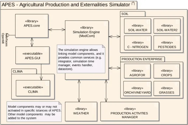
The modelling domain of each component and the subdivision of the modelling system in sub-systems are presented in the following figure, where the main components of APES are shown. To meet the requirements of the system (see 2.1.1) a finer granularity was sometimes chosen, i.e. by subdividing a component into more than one discrete software unit.

APES - Agricultural Production and Externalities Simulator

CLIMA PRODUCTION ENTERPRISE SOIL «library» Simulation Engine (ModCom)

The simulation engine allows linking model components, and it provides common services (e.g. integrator, simulation time manager, events handler, datastore). «library» CROPS «library» WEATHER «library» PESTICIDES

Model components may or may not activated in specific istances of APES. Other model components may be added to the system

«library» PRODUCTION ACTIVITIES MANAGER «library» ORCH/VINEYIARD «library» SOIL-WATER2 «library» SOIL-WATER «library» GRASSES «executable» APES.GUI «library» APES.core Op e n M I In te rf a c e s «library» AGROFOR «library» C - NITROGEN «executable» CLIMA

Fig. 1 APES component diagram. APES is composed of three main groups of software units:

the graphical user interface and the core services component to run Modcom; the simulation engine Modcom, and the model components. Model components can be grouped as soil components, production enterprise components, weather and agricultural management. Note that an alternate option for simulating soil water (SOIL WATER 2) is being developed to provide a first test for components replaceability.

Several criteria have driven the selection of a sub-set of components for prototype 1, starting from time constraints, which forced to concentrate on a subset of actions to maximize chances to match the deadline. Such criteria can be grouped as 1) due to simulation input/output needs, and 2) due to technical needs. Such criteria are listed below.

(15)

1) Criteria due to simulation input/output needs. In SeamFrame, APES is linked to the Production Enterprise Generator, the Production Technique Generator, and the Technical Coefficients Generator (see deliverable 3-2-19). More specifically, the former two provide inputs to APES, whereas the latter uses its outputs. The three generators mention are also under development and needed to test a basic set of inputs (to be supplied to APES) and outputs (to be received from APES). Further, the test cases analyses planned for the first prototypes also required some specific outputs to be transformed in indicators and to be used in the analysis. Consequently, components selection was driven by the need of:

• Make available simulation water and nitrogen limited production;

• Make available simulation of processes which lead to main possible externalities of the system: soil erosion, runoff, nitrogen dynamics in the soil, agrochemicals fate; • Make available the simulation event driven of agricultural management;

• Test links from components beyond the technical aspect, that is, testing the process of building a consistent input-output matrix and using semantically rich interfaces; • Have concrete realizations to discuss criteria for model selection within component

and then component matching

• Provide an articulated example of parameter needs

• Provide an articulated example of models implemented to derive abstractions for model testing, thus leading to designing proper tools for the purpose

2) Criteria due to technical needs. Whether the abstractions and general concepts of a modelling framework are consolidated, moving from simple proofs of concept to actual, articulated applications needs to be tested and worked out not only with respect to implementation details, but also testing aspects related to multi-team work. The criteria for selecting components for prototype 1 consequently were:

• Implement various components to test different types of connections: for instance, all components are connected to agro-management and weather, agro-chemicals and soil carbon-nitrogen needs soil water, crop should be able to run, for potential production, with the weather component only, soil water might be able to simulate a bare soil with the weather components only;

• Link different components from the point of view of matching inputs-outputs from the technical point (e.g. arrays, units) and at various times during simulation (across and within time steps);

• Implement “one per type”, meaning including a crop component (grasses / vineyards / orchards / agroforestry will basically fill the same “slot”), a soil water component (components replaceability will be tested using soil water 2), a soil carbon and nitrogen component, an agro-chemicals component, an agro-management component, a weather component, in order to start:

o Building proper graphical user interfaces (e.g. to show soil profiles for water, nitrogen, agro-chemicals outputs; to test agricultural management configurations input and output);

o Testing input/output procedures (access to input sources, various forms of simulation outputs persistence)

(16)

• Provide articulated samples to allow designing and testing of the relevant part of the knowledge base

• Evaluate the impact of using relatively new IT technologies with teams with different expertise

Within components, beyond what stated in the introduction, a mandatory criteria for model selection is that single models must be peer reviewed to build the foundation of confidence not only in APES, but also in the content of the knowledge base to be built. Developing a component for a specific domain could also be seen as making a review of modelling approaches available as peer reviewed sources, and make them available also for use by third parties. If a new modelling approach is needed because no peer reviewed model is available for a specific purpose, the modellers involved in the project may develop new approaches, in this case submitting a paper to review.

The following section presents the architecture (section 2.1) of the components currently available (section 2.2) as first prototypes, while a third section (section 2.3) presents other components being developed, some already used in the current APES release, others to be included in the coming releases.

2.1 Component architecture

2.1.1 Component requirements

The solution of biophysical modelling problems can be implemented with different designs and different technologies. Developing a design and selecting a technology should be the result of a careful definition of requirements. The requirements below were defined for model components:

Functional requirements

• Estimate/generation of variables via different models; • Estimate parameters from observational data;

• Provide data at run time, accessing either observational or generated data, and making available model outputs;

• Provide quality checks on data imported; • Provide quality checks on outputs produced; Non-functional requirements

• Ease of use: the components must be usable by clients easily: impact on technology and on documentation;

• Extensibility: the capability of easily adding alternate processing capabilities to the ones of the component from the side of the component user, without needing to recompile the component, and using the same interface;

• Reusability: the practical possibility of using the component in different software systems; ease of use and solution to a common modelling problem are the keywords; • Replaceability: the capability of being replaced by a different component respecting

the same contract. “Different” here means either a newer version of the same component, or an implementation from a different party;

(17)

• Documentation: models, software design, code;

• Unit tests: units tests for each public method, input-output tests reported on documentation.

Technological requirements

• Language: C# (.NET platform); • Documentation: HTML-style, PDF.

2.1.2 Ontology

The components contain information extracted from a public ontology. Information consist of concepts (variables in this case, which can be seen as instances of the concepts) and of several attributes for each variable, encapsulated using the VarInfo type available in the Preconditions component (see 2.2.5). The description of the VarInfo type follows, with some comments:

• varName: the name chosen for a variable. The variable name uniquely identifies the variable with its scope. Note that the naming convention used, although sometimes not correct with respect to English, is used to keep similar/related variables close in lists ranked alphabetically. For instance, instead of extraterrestrialRadiation and hourlyExtraterrestrialRadiation, we called the variables extraterrestrialRadiation and extraterrestrialRadiationHourly.

• description: the information to complement what might not be unequivocally understandable from meaningful variable names.

• default value: a default value assigned to the variable. This is used to set up initial conditions (when applicable), or to provide a value for parameters (parameters will have the same metadata structure).

• minValue, maxValue: minimum and maximum values attached to the variable. They are used to restrict the range of variability (in order to prevent the client from using unreasonable values) and perform pre- and post condition tests. Note that a variable may be estimated from other variables via a model. In this case, the minValue and maxValue of the latter variables allows the range of the derived variable to be computed.

• units, varType: units and enumeration types. They are used to link components to the simulation engine, and in case of the units, to perform consistency checks. Among these attributes the properties with respect to data flow are not included as they are not an intrinsic attribute of the variable. In other words, a variable can be an input in a model, and an output in another model.

The use of this information is in the domain classes described below. The components also contain internal information about parameters and variables, using the same VarInfo type. Such information is defined in the component and used as described in the paragraph pre post conditions).

The information above was used to populate a shared ontology, which is implemented in the project as a web based application available at:

http://seamless.idsia.ch/seamontology/chooser/chooser.php?page=Variables

A model interface is defined as a collection of variable definitions. Collections of variables that are associated with particular domains define the Domain Classes (e.g. we could define the SoilDomainClass as the collection of all measurements that are measured on Soil). Such collections can be manually entered by a user or they can be automatically built, using the built-in reasoning features of an ontology. The definition of domain classes in the component

(18)

interface allows abstracting the dependency of the model from the data and fostering the extensibility of models via design patterns.

Having defined a domain class in the ontology, an OWL file can be parsed to generate the source code of the model interface or the domain class respectively. An application to generate C# code of domain classes has been developed (Domain Class Coder,

http://craisci.icamodelling.it/dcc/). Using domain classes, a modeler can exploit the knowledge structured in the ontology in different modeling frameworks or different programming languages. The adoption of an ontology-driven approach for defining a model interface has clear advantages as it enables the reusability of models in a more easy way, while common problems related to poor semantics of model interfaces can be effectively tackled. Currently, the APES ontology is being populated.

2.1.3 Components design

Different designs have being used in the first, exploratory development of components for APES, basically limiting the requirements to the use of a .NET language (all have used C#). The reason was to facilitate as much as possible the development of the first release of APES by taking advantage of work that had already been carried out for a different purpose. The design traits summarized in this paragraph have been adopted, with small differences, in the components described in 2.2.

The general requirement meant to be realized via the design choices made was to produce intrinsically reusable components, that is not targeted specifically to a given modelling framework. To be truly reusable a component must have limited dependencies, be fully documented, and require a modest effort to be re-used. More capabilities could have been obtained, say by making a large use of inheritance; instead, the design chosen makes use of interfaces which specify what a class or the component must do, not how. This increases flexibility which in turn favors replaceability. Also, components are “light-weight”: they do not carry dependencies to whole frameworks to be used. The specific design choices made are briefly discussed in the following paragraphs.

2.1.3.1 Model granularity

A model can be defined as a conceptualization of a process. This is one possible definition of a model, relevant to the work of developing components for biophysical simulation. A model can be implemented in a class, providing the estimation/generation of a variable (or a set of interrelated variables), obtaining a fine level of granularity. There might be more than one way to estimate/generate a variable. If two different models estimate variable A, those two models are alternatives to estimate variable A even if they have different input requirements and different parameters. As a consequence, the two models must be available as separate units, and their input, parameters and output must be defined. Such units are here called “strategies”, from the related design pattern introduced below.

A way to have available in a component all models, via the same call, including alternate approaches, is the implementation of the design pattern Strategy (Mesketer, 2004). The design pattern Strategy offers the user of the component different algorithms by encapsulating them in a class called Context. Different algorithms, which are alternative options to do the same thing, are called, as introduced above, strategies. When building a biophysical model component this allows in principle to offer alternate options to estimate a variable or, more in general, to model a process. This often needed feature in the implementation of biophysical models, if implemented using the design pattern Strategy, comes with two very welcomed benefits from the software side: 1) it allows an easier maintenance of the component, by facilitating adding other algorithms, 2) it allows to add easily further algorithms from the client side, without the need for recompiling the

(19)

component, but keeping the same interface and the same call. The basic point here is that a strategy (a model class) encapsulates a model, the ontology of its parameters, and the test of its pre/post conditions (see 2.1.3.3). It can be used either directly as a strategy (in this case we call it “simple strategy”, where simple indicates that is does not use other strategies as part of its implementation), or it can be used as a unit of composition, as described below.

A composite strategy differs from a simple strategy because it needs other (simple) strategies to provide its output(s). A sequence of calls might be implemented inside a composite class. The list of inputs is given but includes all the inputs of all classes involved (except those which are matched internally). The list of outputs includes all outputs produced by each strategy and the ones specific of the composite class (if any). The list of parameters needed includes the ones of the classes associated and the ones (if any) defined in the composite class; when the value of a parameter is set, if the parameter belongs to an associated class, it is set on that class. The test of pre/post conditions makes use of the methods available in each simple strategy class associated, plus the new tests specified in the composite class. If a violation of pre/post condition occurs in one of the associated classes, the message informs not only about the violation occurred, but also in what class occurred. Composite strategies do not differ in their use compared to simple strategies. An example of simple and composite strategies is given by Villa et al. (2006). Composite strategies too can be added to the components without requiring a re-compilation of their code, thus providing a way to extend component models in full autonomy by third parties. Composite strategies are solutions to modelling problems at a coarser granularity (in principle) with respect to simple strategies. As an example, a composite strategy may be built to simulate “crop potential production” and be developed composing simple strategies such as “light interception”, “crop development”, “leaf area expansion”, etc. In other terms, a composite strategy is a “closed” solution which makes use of selected models of finer granularity as units of composition (simple strategies, see previous paragraph). Such a closed solution is not meant to be proposed as the unique solution for a specific modelling problem. Making reference to the example above about “crop potential production” two composite strategies may use different simple strategies to simulate “light interception” if they target the simulation of either homogeneous canopies or wide-row spacing crops. Whether such diversity in light interception models might not cause noticeable differences in outputs when simulating potential yield, it may lead to sharp differences when simulating water-limited production in arid environments. Further, two alternate approaches to model light interception say for “homogeneous canopies” could be implemented in two composite strategies, and this would allow for comparison of modelling approaches at fine granularity. This kind of composite models will provide a sound foundation to select modeling approaches to be used at operational level.

The formalization of models in basic units of composition (simple strategies) and in aggregated units (composite strategies), providing the same interface, and decoupling interfaces and data from modelling equation as discussed in the next paragraph, provides the design infrastructure to link and populate a knowledge base. The use of semantically rich interfaces fosters safe reusability of components as discussed in the introduction. Finally, simple and composite strategies are discrete units of code which can be directly used either to build components, or even “full” simulation models to be used stand alone, in the latter case still preserving the benefits of a modular system as described in the introduction.

2.1.3.2 Decoupling implementation of interfaces and data from model

equations

Targeting model component design to match a specific interface requested by a modelling framework decreases its reusability. This can partly explain why modeling frameworks,

(20)

although in theory a great advance with respect to traditional model code development, are rarely adopted by groups other than the ones developing them.

A possible way to overcome this problem is to adopt a component design which targets intrinsic reusability and interchangeability of model components (e.g. Donatelli et al., 2004; Donatelli et al., 2005). This may lead, in the worst cases, to the need for a wrapper class (specific to a modeling framework) as proposed by the Adapter pattern (Gamma et al. 1994) that makes possible the migration to other modelling frameworks.

A key design criterion, which enhances reusability and interchangeability, and which allows concurrent development of both components and clients, is separating the model equation component interface and its implementations, in different software units (D’Souza and Wills, 1999; Cheeseman and Daniels, 2000; Löwy, 2003). Self-standing interfaces decouple clients and providers. This is known as the Bridge pattern (Gamma et al., 1994; Mesketer, 2004) and it allows defining units of reusability (model component implementations and model component interfaces) and units of interchangeability (model component implementations alone).

In practical terms related to component development in APES, specifying data-structures (domain classes) for different domains via a shared ontology allows concurrent development of the components which will use their own domain classes and other from other components as parameters in their interface. Once the specific software units with data structures and interfaces are implemented, linking and replacing components can be much simpler (Rizzoli et al., 2005). Such separation is implemented in the AgroManagement, AgrochemicalsFate, SoilWater, and SoilErosionRunoff components (see section 2.2). When the SoilWater2 component (see section 2.3) is available, it will be possible to replace SoilWater with SoilWater2 without requiring any change in other components.

2.1.3.3 Common features of model components

Model components share a set of features to minimize the effort needed to learn how to use them, and to take advantage of common features. For instance, the application Model Component Explorer (see 2.1.4) allows discovering interfaces, domain classes, inputs etc. because of the above mentioned common features.

Pre and post conditions tests

Implementing the test of pre- and post-conditions is the central idea of the Design-by-Contract approach (DBC). In DBC software, entities have obligations to other entities based upon formalized rules between them. A functional specification, or 'contract', is created for each module. Program execution is then viewed as the interaction between the various modules as bound by these contracts. In general, routines have explicit preconditions that the caller must satisfy before calling the routine, and explicit post-conditions that describe the conditions that the routine will guarantee to be true after the routine finishes. When implementing biophysical models, the implementation of the DBC approach not only ensures the correct functionality of the software, but it also specifies what are the limits of use of our model, which is knowledge about the model itself. Also, it allows data of uncertain quality to be used: if an input (either an exogenous variable or the output of another component) is out of the range expected, an exception can be fired, both informing the user of the problem and allowing for exception handling. The DBC approach is implemented via a utility component developed for the purpose, called Preconditions (see 2.2.6).

Unit tests

In computer programming, a unit test is a procedure used to verify a particular module of source code is working properly. The idea about unit tests is to write test cases for all

(21)

functions and methods so that whenever a change causes a regression, it can be quickly identified and fixed. The goal of unit testing is to isolate each part of the program and show that the individual parts are correct. Unit testing provides a strict, written contract that the piece of code must satisfy. Beyond the general benefits which derive from unit tests, implementation in software development, implementing unit tests to test model implementation and making available the relevant input-outputs in the documentation allows the user of the components to have sample application results for the specific model.

Models and software design & use documentation

Each component has a HTML-style help which contains detailed documentation about the models implemented, and information about the design and use of the component. The documentation provided allows re-implementation of all the models of the component, although the characteristics of reusability of the component make it much easier to use, rather than to duplicate it. Another HTML-style file made available for each component is the code documentation, following the standard of the MSDN - .NET documentation.

Exception handling

Exception handling is a programming language construct designed to handle runtime errors or other problems (exceptions) which occur during the execution of a computer program. Handling exceptions is of crucial importance in a component based system as it prevents the system from crashing and it allows users (the applications / subsystems using the components) to know precisely the source of the error. Components handle exceptions and provide a custom message informing users which component and class are the source of the error.

Maximize API ease of use

One of the key elements for component adoption by third parties is the simplicity of default usage cases via the application public interface (API). The usage model for component-oriented design follows a pattern of instantiating a type (a class) with a default or relatively simple constructor, setting some instance properties, and finally, calling some simple instance method. This is called the Create-Set-Call pattern (Cwalina and Abrams, 2006), and it has been implemented in the components. Source code examples for components use provided show example of such usage.

2.1.4 Discovering component and model interfaces

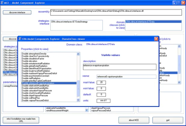
The Model Component Explorer (MCE http://craisci.icamodelling.it/mce/) is a Windows application to inspect model components to discover interfaces, domain classes, VarInfo values, simple and composite strategies, and their parameters, inputs and outputs.

Taking as an example the assembly CRA.clima.et.interfaces.dll in Fig. 2, ETData is a Domain Class and ETDataVarInfo is the relevant VarInfo class. All model strategies are available in the component CRA.clima.et.dll. Currently, not all components can be explored using the MCE).

The interface and the domain classes are discovered by selecting an assembly via the button Discover Interfaces. The screen image of Fig. 2 shows also the content of the Domain Class. Note that by clicking on a property in the list, the VarInfo attributes are shown.

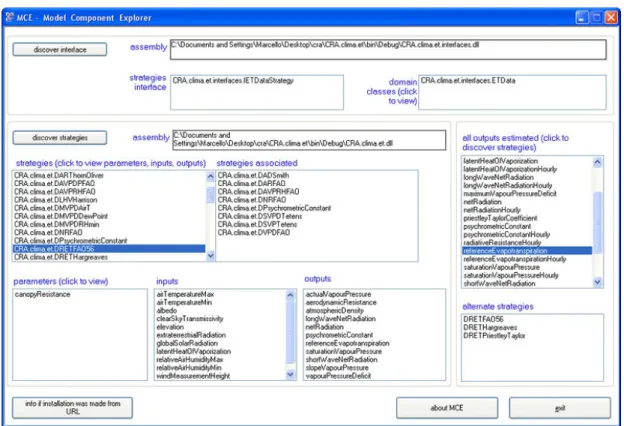
By selecting a model component via the button Discover Strategy, all the strategies are shown, and all outputs produced by the component are also listed. Selecting a strategy causes the display of the relevant parameters, inputs, and outputs. If an output is selected on the list right to the list of the strategies, in the list box below all the strategies (one or more) which produce that output are shown (Fig. 3).

(22)

If a composite strategy is selected (a composite strategy is associated with other strategies), the associated strategies are shown. If the list box associated strategies is empty, that means that the strategy being inspected is a simple strategy. If a parameter is selected, its VarInfo values are shown

Fig. 2 Inspecting domain classes and VarInfo values of a component via the Model

(23)

Fig. 3 Discovering strategies in a model component via the Model Component Explorer.

DREFAO56 is a composite strategy which is built using the simple strategies listed in the box “strategies associated” (see 2.1.3.1 for details).

2.2 Components available

Components available for download include dynamic link libraries, help and code documentation, and source code examples for their use. They are all available for free download via web as specified in appendix B.

All model components implement a dependency to the “impact” data structures of the component AgroManagement (see the following paragraph) to be able to recognize published agro-management events, thus being able to implement the relevant impact.

The following paragraphs contain summaries of the models implemented in the components. Full documentation is available in the PDF version of the help files provided, and it includes the relevant references which are not reported in following summaries to avoid duplication.

2.2.1 AgroManagement

The AgroManagement component is designed to implement production management actions within the system. An agricultural activity is defined, in this context, as a production enterprise (e.g. a crop rotation, an orchard) associated with a production technique (e.g. irrigated, high nitrogen fertilization, minimum tillage). Such an integrated system must be implemented in a way that imitates as closely as possible farmers’ behaviour. Limiting the drivers of the decision making process to the biophysical system implies that each action must be triggered at run time via a set of rules, which can be based on the state of the system, on constraints of resources availability, or on the physical characteristics of the system. However, simulating management in a component-based system poses challenges in defining a framework which must be reusable and able to account for a variety of agricultural

(24)

management technologies applied to different enterprises. Finally, the implementation of management must allow using different approaches to model its impact on different model components.

The AgroManagement component formalizes the decision making process via models called rules, and it formalizes the drivers of the implementation of the impact on the biophysical system via set of parameters encapsulated in data-types called impacts. Each operation must have a rule to be applied at run time; when the rule is satisfied, a set of parameters is made available to model components for the implementation of the impact. The component is easily extendable for both rules (which have the structure of strategies, hence rules encapsulate the attributes for each parameter, allow for testing of pre-conditions, and use the same interface implemented to allow the extensibility of the component) and impacts, so that the use of the AgroManagement component allows different modelling approaches to be used. Furthermore, the information on the biophysical system is passed via a data-type called states, which can also be extended. This is important as the current data-type includes the information needed by the rules currently implemented; newly implemented rules might require further variables which can then be added. The output (in terms of management actions to be applied as resulting from rules evaluated at run-time) drivers, to provide a simulation output (e.g. to output to a text file, to an XML file, and to a database, all currently available) can be fully customized by the user as well by adding new ones without recompiling the component.

The rule-based model is characterized by 3 main sections: • Inputs: states and time

• Parameters (values are compared to rules via the rule model) • A model which returns a true/false output

Rules can be based on relative date or based on a set of state variables and are implemented as a class encapsulating its parameters declaration and test of pre-conditions (this also allows management configuration files to be validated via pre-condition tests).

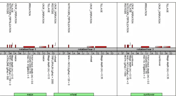
Parameters are needed by model components to implement the impact of management. There are few parameters which are common to a generic management event (e.g. management type) and to a specific management event (e.g. water amount for irrigation, tillage depth for tillage). Other parameters (are needed by specific management approaches (e.g. implement type can be needed by a specific approach to model tillage, as opposed to other approaches to model tillage which do not need such information) and generally at least partially differ even within specific management event types. An example of graphical representation of a management configuration, for a two- years rotation, is shown in the figure below.

(25)

Fig. 4 Graphical representation of agro-management scheduled actions in a two years

rotation. For simulations longer than 3 years the sequence is repeated. Red bars are actions scheduled at a relative (to year) date; red rectangles are actions scheduled in a time window, if other conditions are met; white to red gradient rectangles are actions scheduled with an ending date but associated to a phenological event (the width of gradient boxes is arbitrarily fixed as 30 days in the graphical representation).This type of graphical representation of agro-management configuration files will be available via a specific utility being currently tested.

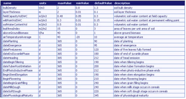
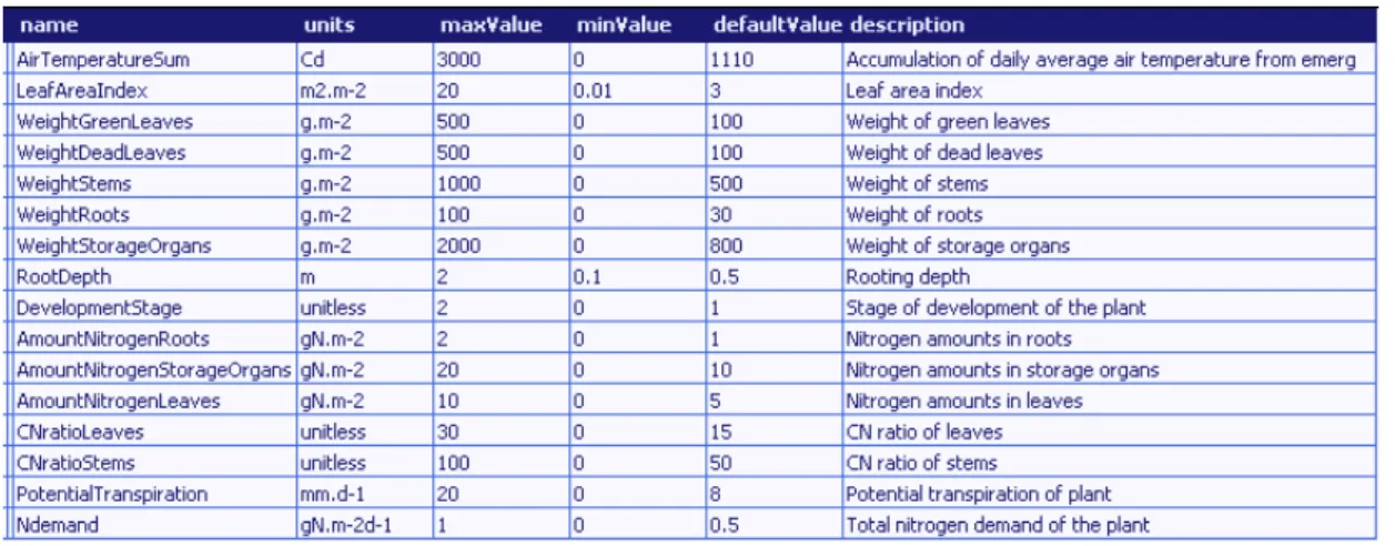
The following table shows the VarInfo attributes of inputs in the use of the component in the release APES v 0.3; rule and impacts parameters are detailed in the documentation and provided via an XML file. Not all dates of phenological events are used in the current version of APES, but the current structure allows for synchronizing management to detail phenological models.

(26)

Table 1 AgroManagement inputs (implementation in APES v 0.3).

2.2.2 AgroChemicalsFate

The AgroChemicalsFate component predicts the fate of agrochemicals in the environment. The model considers 5 compartments where pesticide is stored: canopy surface, plant, available fraction of the soil, aged fraction of the soil and bound fraction of the soil, even though it is possible by strategies to exclude the bound and aged fractions. The available fraction is partitioned in 3 phases: gas, liquid, and solid.

Models are implemented in four composite strategies: • Air

• Crop • Canopy • Soil

The “air” models consider the processes that occur before the pesticide reaches the soil, and they simulate the processes of drift and plant interception.

The differentiation between the virtual compartments “crop” and “canopy” is related to the different processes simulated: on “canopy” the agrochemicals are subject to transformation and can mobilize, whereas “crop” is a sink of agrochemicals. Neither toxicity of accumulated chemicals on the plant, nor the impact on plant products quality, is estimated.

From the surface, the chemical may enter the soil system, transported by infiltrating water and is partitioned among the gas, liquid and solid phases of the soil. The soil compartment is divided in two parts, the first represents the process over the soil surface, the second describes the soil profile. Chemicals are degraded in the soil profile by chemical, photochemical and microbial processes and might be taken up by plant roots.

The component has to be linked to other components to run and to describe the behaviour of pesticides in the modelled system. It is well known that the main determinant of pesticide flow through the soil profile is advection. It is necessary, therefore, that the component reads information about water content and water fluxes from the soil water component. Soil has to provide also temperature because several processes are affected by it. The crop strategy

(27)

requires information about the crop, in particular about ground cover to estimate crop interception of pesticides during application.

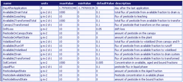
The following tables show the VarInfo attributes of inputs and outputs in the use of the component in the release APES v 0.3.

Table 2 AgrochemicalFate inputs (implementation in APES v 0.3)

Table 3 AgrochemicalFate outputs (implementation in APES v 0.3)

2.2.3 SoilWater and SoilErosionRunoff

The SoilWater component describes the infiltration and redistribution of water among soil layers, the changes of water content, fluxes among layers, the effective plant transpiration and soil evaporation, and the drainage if pipe drains are present. Two algorithms have been selected to simulate the water dynamics, a cascading algorithm and a cascading with travel time among layers. The cascading method simulates the soil as a sequence of tanks that have a maximum and a minimum level of water, fixed respectively at the field capacity (FC) and wilting point (WP). Water in excess of the water content at FC for a given layer is routed into the lower layer, and if all the profile has reached FC, the water in excess is removed from the soil as percolation. The main advantage of this approach is the simplicity and the calculation speed. The main difficulties are that the model has not a strong physical background, because the concept of field capacity is a practical approximation and represents a simplification of soil water holding features, and because the time needed to water to move between layers is not considered. Other relevant difficulties of this approach is the impossibility to have soil

(28)

water contents greater than FC and lower than WP (the latter with exception of the evaporative layer), and the possibility to have allowed movement of water only downwards. This approach is not suitable where there are layers of different texture or a water table, even if it is possible to use some approximation to simulate the capillary rise. The cascading method with travel time is an extension of the simple cascading method, taking into account the time needed to percolate the layer. Tillage simulation is done following the approach of the models Wepp and SWAT, where each type of equipment used on the soil has specific parameters and a coefficient for the intensity of tillage (mixing among layers), for surface roughness after tillage, ridge high and distance This allows for the simulation of the evolution of bulk density in time, because a simple model of soil settling after tillage was also developed. Currently, all the variables are simulated with a daily time step, but the algorithms and software structure are ready to work with an hourly or shorter time step.

The SoilErosionRunoff component simulates dynamically water runoff and soil erosion. In detail, it represents the runoff volume, the amount of soil eroded, the interception by vegetation, and the water available for infiltration. This component has been structured in a hierarchical way with the above-described Water component, but has its own data-type and related interfaces. As for the Water component, all the variables are simulated using a daily time step, but the algorithms and software structure are already designed to work with an hourly or shorter time step.

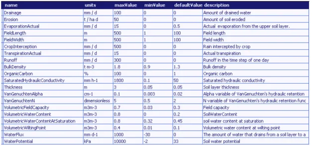
The following tables show the VarInfo attributes of inputs and outputs in the use of the component in the release APES v 0.3.

Table 4 SoilWater/ErosionRunoff inputs (implementation in APES v 0.3)

(29)

2.2.4 Weather

Weather components implement several strategies, from peer reviewed sources, to estimate variables subdivided in five domains. Emphasis is placed in sharing and making available for operational use modelling knowledge produced by research. Weather components can be considered as a realization of a part of “Numerical recipes in agro-ecology” as proposed by Leffelaar et al. (2003), implemented using an updated technology. The reason for the subdivision in components is to make it easier to re-use and maintain the models. The reference to the peer reviewed sources of the models is available in the documentation.

2.2.4.1 AirTemperaure

The generation of daily maximum (Tmax, °C) and minimum (Tmin, °C) air temperatures is considered to be a continuous stochastic process with daily means and standard deviations, possibly conditioned by the precipitation status of the day (wet or dry). Three alternative methods are implemented for generating daily values of Tmax and Tmin, all based on the assumption that air temperature generation is a weakly stationary process. The multi-stage generation system is conditioned on the precipitation status with two approaches. Residuals for Tmax and Tmin are computed first, than daily values are generated - independently (Richardson-type) or with dependence of Tmax on Tmin (Danuso-type). A third stage, that adds an annual trend calculated from the Fourier series, is included in Danuso-type generation. Another approach even accounts for air temperature-global solar radiation correlation. A third approach generates Tmax and Tmin independently in two stages (daily mean air temperature generation first, Tmax and Tmin next), making use of an auto-regressive process from mean air temperatures and solar radiation parameters. Daily values of Tmax and Tmin are used to generate hourly air temperature values, according to alternative methods. Sinusoidal functions are largely used to represent the daily pattern of air temperature. Six approaches, are used to generate hourly values from daily maximum and minimum temperatures. A further approach derives hourly air temperatures from the daily solar radiation cycle. Mean daily values of dew point are estimated via empirical relationships with Tmax and Tmin and other variables. A diurnal pattern (hourly time step) of dew point is also modelled via two alternative methods.

2.2.4.2 Evapotranspiration

Evapotranspiration for a reference crop (ET0) is calculated from alternative sets of inputs and for different canopies, conditions and time steps, using one-dimensional equations based on aerodynamic theory and energy balance. A standardized form of the Penman-Monteith equation is used to estimate daily or hourly ET0 for two reference surfaces. According to FAO Irrigation and Drainage Paper n. 56, the reference surface is a 0.12-m height (short crop), cool-season extensive grass such as perennial ryegrass or tall fescue . A second reference surface, recommended by the American Society of Civil Engineers, is given by a crop with an approximate height of 0.50 m (tall crop), similar to alfalfa. The Priestley-Taylor equation is useful for the calculation of daily ET0 for conditions where weather inputs for the aerodynamic term (relative humidity, wind speed) are unavailable. The aerodynamic term of the Penman-Monteith equation is replaced by a dimensionless empirical multiplier. As an alternative when solar radiation data are missing, daily ET0 can be estimated using the Hargreaves equation. An adjusted version of this equation, according to Allen et al. is given. Stanghellini revised the Penman-Monteith model to represent conditions in greenhouse, where air velocities are typically low (<1.0 m s-1_{). A multi-layer canopy is considered to} estimate hourly ET0, using a well-developed tomato crop, grown in a single glass, Venlo-type greenhouse with hot-water pipe heating. The Stanghellini model includes calculations of the solar radiation heat flux derived from the empirical characteristics of short wave and long

(30)

wave radiation absorption in a multi-layer canopy. A leaf area index is used to account for energy exchange from multiple layers of leaves on greenhouse plants. The constituent equations of the Stanghellini model are in accordance with the standards of the American Society of Agricultural Engineers.

2.2.4.3 Rain

The occurrence of wet or dry days is considered to be a stochastic process, represented by a first-order Markov chain as described by Nicks et al. The transition from one state (dry or wet) to the other (dry or wet) is governed by transition probabilities, as characterized monthly by analyzing historic long-term daily precipitation data for the site. According to the multi-transition model of Srikanthan and Chiew, the daily precipitation amounts are divided into up to seven states - dry or wet from 1 (lowest rainfall) to 6 (highest rainfall). On days when precipitation is determined to occur the precipitation amount is generated by sampling from alternative probability distribution functions. Most approaches are based on the two-state transition model for dry/wet days. The Gamma distribution is used to model precipitation amounts for the last state (highest level of rainfall) in the multi-state transition probability matrix of Srikanthan and Chiew, while a linear distribution is applied for the other states. The pattern of Gamma plus linear distribution across various occurrence states exhibits a combined J shaped function.

Short-time rainfall data are generated by disaggregating daily rainfall into a number of discrete events, then deriving the characteristics (amount, duration and starting time) for each event. Four approaches have been implemented to disaggregate daily rainfall into six hour or shorter periods (as small as 10 minutes). The method described by Arnold and Williams uses a 0.5-hour time resolution and assumes that daily rainfall falls in only one event. The peak location is generated first according to a broken linear distribution. The other 0.5-hourly amounts are generated from an exponential distribution and relocated on both sides of the peak. The other methods are more flexible and able to capture bursts of storm occurring discontinuously over the day. In the approach by Meteoset an autoregressive process and a Gaussian daily profile model are combined to simulate the possibility of precipitation at any hour. Two options are available to generate sub-daily precipitation events for varying time steps. The cascade-based disaggregation method of Olsson breaks each time interval into two equally sized sub-intervals. The total amount is redistributed into two quantities according to two multiplicative weights from a uniform distribution: 24-hour rain into two 12-hour amounts, 12-hour amount into 6-hour amounts, and so on until 1.5-hour resolution is achieved. The approach by Connolly et al. allows disaggregation of daily rainfall into multiple events on a day, and the simulation of time-varying intensity within each event: (1) distinct storms are assumed independent random variables from a Poisson distribution, (2) the storm origins arrive according to a beta distribution, (3) storms terminate after a time that is simulated by a simplified gamma distribution, (4) each storm intensity is a random value exponentially distributed, (5) time from the beginning of the event to peak intensity is given by an exponential function, (6) peak storm intensity for each event is also determined from an exponential function, (7) internal storm intensities are represented by a double exponential function.

2.2.4.4 SolarRadiation

Solar radiation outside the earth’s atmosphere is calculated at any hour using routines derived from the solar geometry. Daily values are an integration of hourly values from sunrise to sunset. The upper bound for the transmission of global radiation through the earth’s atmosphere (i.e., under conditions of cloudless sky), can be set to a site-specific constant or estimated daily by diverse methods.