New statistical methods to assess the effect of time-dependent exposures in case-control studies

New statistical methods to assess the effect of time-dependent

exposures in case-control studies

par

Zhirong Cao

Faculté de médecine

Mémoire présenté à la Faculté des études supérieures en vue de l’obtention du grade de maîtrise

en sciences biomédicales

Décembre, 2008

Université de Montréal

Faculté des études supérieures

Ce mémoire intitulé

New statistical methods to assess the effect of time-dependent

exposures in case-control studies

présenté par

Zhirong Cao

a été évalué par un jury composé des personnes suivantes :

Président-rapporteur : Jean Lambert

Directeur de recherche : Karen Leffondré

Membre du jury: Andrea Benedetti

First of all, I would like to express my deepest gratitude to my supervisor, Dr. Karen Leffondré, who gave me endless support, intense supervision, and patience. She has always been encouraging and helping me through my graduate study. I would not have completed my study without her help.

I would like to thank Willy Wynant. I thank you for your friendly advices, encouragement and reviewing my thesis.

Thanks are due to Dr. Jack Siemiatycki for his insightful discussion in epidemiology.

I would also like to thank Jerome Asselin for his consistently immediate assistance with technical details and data management issues.

I would like to acknowledge the financial support in the form of scholarships from the National Sciences and Engineering Research Council of Canada (NSERC), Canadian Institutes for Health Research (CIHR), and the Fonds de la Recherche en Santé du Québec (FRSQ).

Last, but not least, I would like to dedicate this thesis to my parents, my husband and my children, for their love, patience, and understanding—they allowed me to spend most of the time on this thesis.

Résumé et mots clés

Contexte. Les études cas-témoins sont très fréquemment utilisées par les

épidémiologistes pour évaluer l’impact de certaines expositions sur une maladie particulière. Ces expositions peuvent être représentées par plusieurs variables dépendant du temps, et de nouvelles méthodes sont nécessaires pour estimer de manière précise leurs effets. En effet, la régression logistique qui est la méthode conventionnelle pour analyser les données cas-témoins ne tient pas directement compte des changements de valeurs des covariables au cours du temps. Par opposition, les méthodes d’analyse des données de survie telles que le modèle de Cox à risques instantanés proportionnels peuvent directement incorporer des covariables dépendant du temps représentant les histoires individuelles d’exposition. Cependant, cela nécessite de manipuler les ensembles de sujets à risque avec précaution à cause du sur-échantillonnage des cas, en comparaison avec les témoins, dans les études cas-témoins. Comme montré dans une étude de simulation précédente, la définition optimale des ensembles de sujets à risque pour l’analyse des données cas-témoins reste encore à être élucidée, et à être étudiée dans le cas des variables dépendant du temps.

Objectif: L’objectif général est de proposer et d’étudier de nouvelles versions du

modèle de Cox pour estimer l’impact d’expositions variant dans le temps dans les études cas-témoins, et de les appliquer à des données réelles cas-témoins sur le cancer du poumon et le tabac.

Méthodes. J’ai identifié de nouvelles définitions d’ensemble de sujets à risque,

potentiellement optimales (le Weighted Cox model and le Simple weighted Cox

model), dans lesquelles différentes pondérations ont été affectées aux cas et aux

témoins, afin de refléter les proportions de cas et de non cas dans la population source. Les propriétés des estimateurs des effets d’exposition ont été étudiées par simulation. Différents aspects d’exposition ont été générés (intensité, durée, valeur cumulée d’exposition). Les données cas-témoins générées ont été ensuite analysées avec différentes versions du modèle de Cox, incluant les définitions anciennes et nouvelles des ensembles de sujets à risque, ainsi qu’avec la régression logistique conventionnelle, à des fins de comparaison. Les différents modèles de régression ont ensuite été appliqués sur des données réelles cas-témoins sur le cancer du poumon. Les estimations des effets de différentes variables de tabac, obtenues avec les différentes méthodes, ont été comparées entre elles, et comparées aux résultats des simulations.

Résultats. Les résultats des simulations montrent que les estimations des nouveaux

modèles de Cox pondérés proposés, surtout celles du Weighted Cox model, sont bien moins biaisées que les estimations des modèles de Cox existants qui incluent ou excluent simplement les futurs cas de chaque ensemble de sujets à risque. De plus, les estimations du Weighted Cox model étaient légèrement, mais systématiquement, moins biaisées que celles de la régression logistique. L’application aux données réelles montre de plus grandes différences entre les estimations de la régression

logistique et des modèles de Cox pondérés, pour quelques variables de tabac dépendant du temps.

Conclusions. Les résultats suggèrent que le nouveau modèle de Cox pondéré propose

pourrait être une alternative intéressante au modèle de régression logistique, pour estimer les effets d’expositions dépendant du temps dans les études cas-témoins

Mots clés. Modèle de Cox pondéré, variables dépendant du temps, étude cas-témoins, régression logistique, exposition cumulée, intensité d’exposition, simulation, tabac, cancer.

Summary and keywords

Background: Case-control studies are very often used by epidemiologists to assess

the impact of specific exposure(s) on a particular disease. These exposures may be represented by several time-dependent covariates and new methods are needed to accurately estimate their effects. Indeed, conventional logistic regression, which is the standard method to analyze case-control data, does not directly account for changes in covariate values over time. By contrast, survival analytic methods such as the Cox proportional hazards model can directly incorporate time-dependent covariates representing the individual entire exposure histories. However, it requires some careful manipulation of risk sets because of the over-sampling of cases, compared to controls, in case-control studies. As shown in a preliminary simulation study, the optimal definition of risk sets for the analysis of case-control data remains unclear and has to be investigated in the case of time-dependent variables.

Objective: The overall objective is to propose and to investigate new versions of the

Cox model for assessing the impact of time-dependent exposures in case-control studies, and to apply them to a real case-control dataset on lung cancer and smoking.

Methods: I identified some potential new risk sets definitions (the weighted Cox model and the simple weighted Cox model), in which different weights were given to

cases and controls, in order to reflect the proportions of cases and non cases in the source population. The properties of the estimates of the exposure effects that result from these new risk sets definitions were investigated through a simulation study.

Various aspects of exposure were generated (intensity, duration, cumulative exposure value). The simulated case-control data were then analysed using different versions of Cox’s models corresponding to existing and new definitions of risk sets, as well as with standard logistic regression, for comparison purpose. The different regression models were then applied to real case-control data on lung cancer. The estimates of the effects of different smoking variables, obtained with the different methods, were compared to each other, as well as to simulation results.

Results: The simulation results show that the estimates from the new proposed

weighted Cox models, especially those from the weighted Cox model, are much less biased than the estimates from the existing Cox models that simply include or exclude future cases. In addition, the weighted Cox model was slightly, but systematically, less biased than logistic regression. The real life application shows some greater discrepancies between the estimates of the proposed Cox models and logistic regression, for some smoking time-dependent covariates.

Conclusions: The results suggest that the new proposed weighted Cox models could

be an interesting alternative to logistic regression for estimating the effects of time-dependent exposures in case-control studies.

Keywords: Weighted Cox model, time-dependent variables, case-control study, logistic regression, cumulative exposure, exposure intensity, simulation, smoking, cancer.

Table of contents

Acknowledgements... iii

Résumé et mots clés... iv

Summary and keywords... vii

Table of contents... ix

List of tables... xi

List of figures... xiii

List of acronyms and abbreviations ... xiv

1

Introduction...1

2

Literature review...4

2.1 Overview of epidemiological study design... 5

2.2 Overview of logistic regression ... 7

2.3 Overview of survival analysis... 9

2.3.1 Survival and hazard functions... 9

2.3.2 Parametric survival models... 10

2.3.3 The Cox semi-parametric model... 12

2.3.4 Adaptation of Cox’s model to case-control study... 15

3

Objectives ...19

4

Methods...22

4.1 New proposed Cox models ... 23

4.2 Simulation study ... 27

4.2.1 Overview... 27

4.2.2 Generation of the source population ... 27

4.2.3 Simulation of case-control studies... 30

4.2.5 Data analytical models... 33

4.2.6 Summary statistics to evaluate the performance of the different analytical models ... 34

4.3 Real data analysis:... 35

4.3.1 Data source... 35

4.3.2 Method to handle missing smoking data ... 36

4.3.3 Description of smoking intensity trajectories over time ... 39

4.3.4 Data analytical models... 41

5

Results...49

5.1 Results from simulations... 50

5.2 Results from real data analysis ... 54

5.2.1 Description of real data... 54

5.2.2 Patterns of smoking intensity... 56

5.2.3 Results from regression models... 58

6

Conclusion and discussion ...66

7

References...71

8

Appendix...75

8.1 Questionnaire on smoking ... 76

List of tables

Table I. Characteristics of the Exponential, Weibull, and Gompertz distributions . .. 11 Table II: definitions of weights in risk sets of models used for subject j at risk at aget_i

: ... 26 Table III : Summary of simulation scenarios in Model 1, hazard depended on

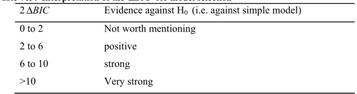
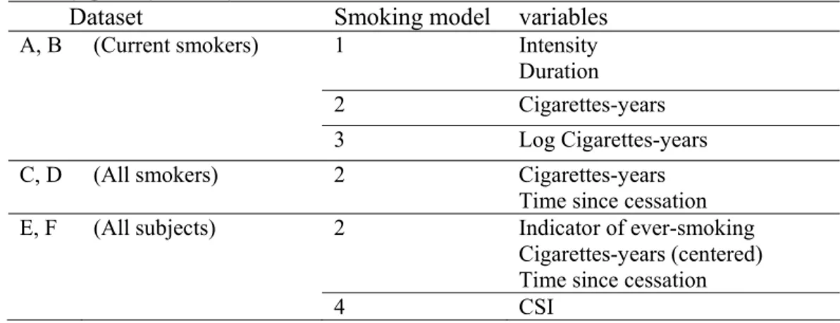
intensity and past duration separately... 32 Table IV: Summary of simulation scenarios for Model 2, where the hazard depended on the value cumulative exposure*... 32 Table V: Summary of smoking variables in the case-control study, Montréal, Quebec, Canada, 1996-2001. ... 36 Table VI: Comparison of the distribution of smoking intensities (n, mean, standard deviation) before and after imputation to handle missing smoking intensity at each of the four ages (25, 40, 50, 60 years) in the case-control study, Montréal, Quebec, Canada, 1996-2001. ... 38 Table VII : interpretation of logged Bayes factor (2 BIC_Δ ) for model selection ... 41 Table VIII: Summary of sub-datasets from a case-control study, Montréal, Quebec, Canada, 1996-2001. ... 42 Table IX: Summary of the smoking models used to analyse the data from the case-control study, Montréal, Quebec, Canada, 1996-2001. ... 45 Table X: lifetime probability of developing lung cancer and probability of developing lung cancer within the next 10 years by age group, Canada... 46 Table XI: Age-conditional probabilities of developing lung cancer in the future and the weights for each age categorical for weighted Cox model in the analysis of

Montreal case-control study... 47 Table XII: Results from simulations of the proposed Cox models and conditional logistic regression (CLR) for estimating the effects _βof intensity I(t) and duration

D(t) (Model 1), based on the 1000 simulations. ... 52 Table XIII: Results from simulations of all the Cox models and conditional logistic regression (CLR) for estimating the effect βof cumulative exposure† (Model 2), based on 1000 simulations... 53

Table XIV: Demographic characteristics of subjects at the time of

diagnosis/interview, Montréal, Quebec, Canada, 1996-2001. ... 54 Table XV: Smoking-related characteristics of subjects in a case-control study of environmental exposure and cancer at the time of diagnosis/interview, Montréal, Quebec, Canada, 1996-2001... 55 Table XVI: Percentages of patterns of intensity change over-time for current smokers in a case-control study, Montréal, Quebec, Canada, 1996-2001. ... 58 Table XVII: Smoking effect estimates from the Cox models and standard

unconditional logistic regression (LR), using Model 1 in current smokers, Montréal, Quebec, Canada, 1996-2001... 63 Table XVIII: Smoking effect estimates from the Cox models and standard

unconditional logistic regression (LR), using Model 2, Montréal, Quebec, Canada, 1996-2001. ... 64 Table XIX: Smoking effect estimates from the Cox models and standard

unconditional logistic regression (LR), using Models 3 and 4, Montréal, Quebec, Canada, 1996-2001. ... 65 Table XX: Questions that were asked in the questionnaire regarding smoking history in the case-control study of lung cancer, Montréal, Quebec, Canada, 1996-2001. .... 76 Table XXI. Mean of the 1,000 estimates, corresponding confidence interval, and relative bias for the adapted Cox model and conditional logistic regression. ... 77

List of figures

Figure 1: Different patterns of smoking intensity change over time for three

hypothetical subjects who have the same value of cigarette-years... 3 Figure 2 : Exposure pattern of a hypothetical subject j diagnosed or selected at age tj,

with an increasing intensity over lifetime... 28 Figure 3: The intensity at different age represented by the intensity at the reported age... 36 Figure 4: make up of the intensity at some age with missing data ... 38 Figure 5: Trajectory of intensity for current male smokers in a case-control study, Montréal, Quebec, Canada, 1996-2001. ... 56 Figure 6: Trajectory of intensity for current female smokers in a case-control study, Montréal, Quebec, Canada, 1996-2001. ... 57

List of acronyms and abbreviations

CSI comprehensive smoking index CCDPC Centre for Chronic Disease Prevention and Control CLR Conditional logistic regression LR logistic regression

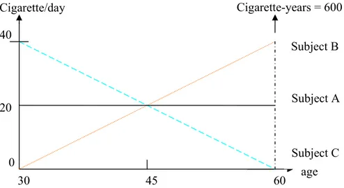
Case-control studies, which consist in sampling subjects who have the disease of interest (the cases) and subjects free of disease (the controls) at the time of study, are very often used by epidemiologists to assess the impact of specific past exposure(s) on the disease of interest[1]. Many of these exposures such as smoking history may be represented by several time-dependent covariates [2], and new methods are needed to accurately assess their effects. Indeed, conventional logistic regression, the standard method to analyze case-control data, does not directly account for changes in covariate over time. For example, in studies investigating the impact of smoking, smoking history is often represented in the regression model by a cumulative exposure variable, cigarette-years, which is the product of 1) the average smoking intensity over lifetime, and 2) the total duration of smoking at the time of diagnosis for cases and at the time of interview for controls. Such a cumulative variable does not allow discrimination between subjects who indeed have cumulated the same amount of smoking, but who smoked with different patterns of intensity over lifetime, as illustrated with the three different hypothetical patterns in Figure 1. In this figure, the three subjects have cumulated 600 cigarette-years over their lifetime, but with very different patterns of intensity over time. Using cigarette-years in a standard logistic regression model to represent smoking history would assume that these three subjects have exactly the same risk of developing the disease at the age of 60 years, with respect to their past smoking consumption. However, since the effect of cigarettes smoked t years ago is likely to decrease as t increases [3], one could assume that subject B with increasing intensity has probably a higher risk at the age of 60,

compared to subject C who has decreasing intensity. By contrast, at ages earlier than 45 years, one could assume that subject B had a lower risk than subject C.

Such patterns over lifetime are difficult to model in a standard logistic regression model. One possibility could be using different variables to represent different periods of past exposures. However, one would have then to face with the problem of arbitrary choice of these periods, and potential multi-colinearity between the resulting covariates. By contrast, survival analytic methods such as the Cox proportional hazards (PH) model [4] can directly incorporate time-dependent covariates representing the individual entire exposure history. However, these methods were originally proposed for prospective data, and their application to retrospective designs requires some careful manipulation of risk sets [5, 6]. The optimal definition of risk sets for the analysis of case-control data remains unclear and has to be investigated in the case of time-dependent variables [7].

Figure 1: Different patterns of smoking intensity change over time for three hypothetical subjects who have the same value of cigarette-years.

Cigarette/day 40 0 30 45 60 20 age Cigarette-years = 600 Subject A Subject C Subject B

2.1 Overview of epidemiological study design

Two important types of epidemiological studies for generation hypotheses are cohort studies and case-control studies. The principles of these two epidemiological designs are briefly outlined below (for more details see e.g. [8] and [9]).

Cohort studies

In a cohort study, a group of individuals who are exposed to a certain condition are followed over time, and compared with another group unexposed to that condition. One measure of interest is the incidence rate, which is number of new disease cases per population at risk. The incidence rates for exposed and non-exposed subjects are calculated separately. The relative risk is the ratio of the incidence rate of exposed subjects to non-exposed subjects and is used to measure the association between exposure and disease.

Population based case-control studies

In a case-control study, subjects with the event/disease (cases) are selected, and then the history of exposure and/or other characteristics is recorded by interview or any other sources. A comparison group (control group) of subjects without the event/disease is assembled from the source population, and the history of controls is recorded as well as for cases. In these studies, individuals with the disease (the cases) are over-sampled. Thus, the percentage of people who has disease is greater in the study than in the source population. The percentage of subjects with the disease in the source population can not be estimated from a case-control study, so the relative risk can not be estimated. However, the odds ratio (OR) can always be estimated in a

case-control study. For a rare disease, the odds ratio (OR) approximates relative risk. Matching between cases and controls is sometimes performed in case-control studies. This ensures that the matchingfactors, such as age or sex, are equally distributed between cases and controls [10]. Both individual matching (one or more controls matched to each specified case) and frequency matching (groups of controls matched to groups of cases) are used.

Nested case-control studies

Since collecting covariate information for all individuals in a cohort may be very expensive, and time-consuming, Langholz [5] shows that the nested case-control design, which is cohort sampling design, is a useful alternative to a full cohort study. Nested case-control studies are case-control studies done in the population of an ongoing cohort study. The case-control study is thus said to be “nested” inside the cohort study. In the nested case-control design, each case is compared to a small sample of individuals (controls) selected form the risk set at the time of case’s event. The collection information includes all cases and only the sampled controls.

Advantages and disadvantages of cohort and case-control studies

Cohort studies allow complete information on the subject’s exposure(s), and estimate incidence rates as well as relative risk. Since cohort studies need a large number of subjects to follow up, they are expensive to carry out and are not suited for rare diseases study. Case-control studies are relatively inexpensive as compared with

cohort studies, so they permit the studies of rare diseases. However, the information on past exposure is usually based on interview, and may be prone to measurement errors because of recall bias. Nevertheless, many case-control studies collect huge information on past exposures, and appropriate statistical methods are needed to account for all this information.

While cohort studies are often analysed using survival analyses methods, case-control data are almost always analysed using logistic regression. In the following sections, I briefly present these two analytical approaches.

2.2 Overview of logistic regression

Logistic regression is a part of generalized linear models [11]. Logistic regression allows the investigation of the relationship between a binary response variable Y, such as presence/absence or success/failure, and a set of explanatory variables X. The outcome variable Y follows a Bernoulli distribution with a probability of “success” P(Y=1|x)= _{π(x), which is given by :}

) ' exp( 1 ) ' exp( ) ( X X x β α β α π + + + = (2.1)

where α is the intercept and β is the vector of regression coefficients. Equation 2.1 can also be written:

∑

+

=

+

=

⎥

⎦

⎤

⎢

⎣

⎡

−

=

x

X

x

x

x

'

)

(

1

)

(

ln

)

(

logit

α

β

α

β

π

π

π

which shows that the logistic regression model assumes that the effects of all Xj are

linear on the logit of _{π. For each X}j, exp(βj) corresponds to the OR for Xj. The latter

result explains the popularity of logistic regression in epidemiology.

Let y be the indicator, taking the value 1 if the subject i has the event, and 0 _i

otherwise. The regression coefficients are estimated by maximizing the likelihood function:

[

]

∏

Note that Prentice showed that we can analyze retrospective data as if they were prospective [12].

Conditional logistic regression

Conditional logistic regression is used to analyse individually matched case-control studies. Conditional logistic regression works in nearly the same way as regular logistic regression, except one needs to specify which individuals belong to which matched set (i.e. strata).

The theory is similar: one can derive a conditional likelihood and maximize it. From a practical perspective, the only difference is the need to specify the matched set to which each person belongs. When each matched set consists of a single case and a single control, the conditional likelihood is given by:

(

)

[

]

(

)

[

]

∏

where xi1 and xi0 are the vectors of explanatory variables of the case and the control,

respectively, of the ith matched set.

2.3 Overview of survival analysis

Survival analysis is a popular data analytical approach for studies in which outcome variable of interest is time until an event occurs (referred to as time-to-event). Time means years, months, or days from the beginning of follow-up of a subject until an event occurs; alternatively, time can also refer to the age of a subject when an event occurs. Event means death, disease incidence, recovery (e.g. return to work) or any designated experience of interest that may happen to a subject.

Censoring is a key analytical problem in survival analysis, since one may ignore the survival time for some subjects. Censoring may occur when a person does not experience the event before the study ends, or a person is lost to follow-up during the study period. There are three types of possible censoring schemes, right censoring, interval censoring and left censoring. All along this thesis, I consider only the case of right censoring.

2.3.1 Survival and hazard functions

Let the random variable T denotes the survival time, and f(t) its density probability function:

t t t T t P t f t Δ Δ + < ≤ =_Δlim_→ ( ) ) ( 0 (2.5)

F(t) denotes the cumulative distribution function

). ( )

(t PT t

F _{= ≤} (2.6) The survival functionS(t) is therefore written

) ( 1 ) ( ) (t P T t F t S _{= > = −} . (2.7) The hazard function h(t) is given by

) ( ) ( ) | ( lim ) ( 0 St t f t t T t t T t P t h t Δ = ≥ Δ + < ≤ = → Δ . (2.8)

h(t)_Δt is the probability to have the event of interest between t and t + _Δt,

conditionally on being still at risk at time t, i.e. not having experienced the event before t. The cumulative hazard function is finally given by

∫

. )) ( log( ) ( ) ( ' ) ( ) ( ) ( dt t S d t S t S t S t f t h = =− =− (2.10)

2.3.2 Parametric survival models

When using parametric survival models, one assumes that the survival time variable T follows a known distribution that depends on a finite number of unknown parameters. The most popular distributions are the Exponential distribution, the Weibull distribution and the Gompertz distribution. Table I gives their characteristics [13].

Maximum likelihood estimation is used to estimate the unknown parameters of the parametric distributions. Let ti be the survival or censoring time of subject i, and di

the indicator, taking the value 1 if the subject i has the event at time ti, and 0

otherwise. The likelihood function under general non-informative censoring has the form ( )

∏

=

x

S

t

x

t

f

L

)

(

)

(

)

(

_θ

Table I. Characteristics of the Exponential, Weibull, and Gompertz distributions [13].

Distribution

Characteristic Exponential Weibull Gompertz Parameter Scale parameterλ>0 Scale parameterλ>0

Shape parameter v>0 Scale parameterλ>0 Shape parameter ) , (_{−∞ ∞} ∈ α Hazard function h0(t)=t 0( )= −1 v vt t h λ h0(t)=exp(αt) Cumulative hazard function t t H₀( )_{=λ H (t)=λt}v 0 0( )=α (exp(αλ)−1) λ t H Density function ) exp( ) ( 0 t t f _{=λ −λ} ) ( ) ( 1 0 v v _{esp t} vt t f λ λ − =

− exp( )exp( (1 exp( )

) ( 0 αλ α λ αλ λ − = t f Survival

function S₀(t)₌exp(_−λt) _S0(_t) _esp( _tv)

λ − = 0() exp( (1 exp(αλ) αλ − = t S

2.3.3 The Cox semi-parametric model

Since it is difficult to specify a priori correct assumption concerning the nature or the shape of the underlying survival distribution as required with parametric approaches, the Cox semi-parametric model is rather used in practice. This proportional hazards (PH) model, which was introduced by Cox [4], is the most popular regression model used for analyzing survival data. It consists in a product of a term depending on time and a term depending on the covariates

) ' exp( ) ( ) (tx h₀ t x h _{= β} (2.12) where X=X₁,X₂,...,X_p is the vector of the p explanatory/predictor variables, and

) ( 0 t

h the baseline hazard function, which does not have to be specified. The Cox model is a semi-parametric model because of the non parametric function h₀(t) and the parametric function exp( x_β' ).

The most important feature of the model is the proportional hazards (PH) assumption. Let consider two subjects i and j who differ in their covariates value for x1, but have

the same value for other covariates. The hazard ratio for x1 between these two

subjects will be

(

)

[

]

exp

x

x

HR

₌

_β

₋

time. That is why the Cox model is called the PH model. Note that the variables can be time-dependent as explained below. What can’t be time-dependent with the PH assumption is their effect _β.

Partial likelihood

The regression parameters in the Cox PH model are estimated by maximizing a partial likelihood, developed by Cox [4, 14]. The Cox partial likelihood is based on the observed order of events and is constructed by comparing the hazard of the subject i who fails at time ti to the hazard of all subjects j at risk just before that time ti. The Cox partial likelihood is given by

( )

_{∏ ∑}

(

₍

)

₎

β

β

β

where Ri is the risk set at time ti made of the group of subjects at risk for failure just

before ti. The above equation is correct if no ties occur at any of the failure times, i.e.

each failure occurs at a distinct time. We can use either Breslow [15] or Efron [16] approximations if there are ties in the data set, since the exact method can be time-consuming.

Extension of the Cox PH model for time-dependent variables

The values of some covariates, such as intensity of exposure, may change over time for some subjects. Covariates can thus be either fixed or time-dependent. It is possible to incorporate time-dependent covariates in the Cox model:

( )

( )

[

( )

]

h _{= 0}( )exp _β' (2.15) Note that such a model no longer satisfies the “strict” PH assumption and is sometimes called extended Cox model, see Fisher [17]. However, even if a covariate is time-dependent, its effect _{β may be constant over time, which is in agreement with}

the PH assumption. The regression coefficients can be estimated through the time-dependent partial likelihood [18].

( )

_{∏ ∑}

(

₍

( )

_{( )}

)

₎

β

β

β

In Cox’s model, the time axis (or time-scale) T, has to be defined when we build the risk sets. Many authors have frequently used time-on-study or calendar time as the time-scale, because Cox’s model was developed originally for clinical applications, where individuals are generally followed up since the initiation of treatment until death. However, a previous simulation study [19] that simulated cohort data, showed positive bias for dependent covariates when using on-study as the time-scale, and when the baseline hazard was not an exponential function of age [19]. By contrast, no bias was observed when using age as the time-scale.

In many epidemiological studies, the effect of age needs to be tightly controlled because the incidence of the disease of interest depends strongly on age. This is the case for example in aging research. In such situations, using age as the time-scale allows direct adjustment for age, without having to model its effect with any linear function or arbitrary categorization. Note that in aging research, using age as the time-scale often requires left truncation [20]. For example, if the objective of the study is to investigate the risk of dementia as a function of age, the age at dementia

should be left-truncated if subjects enter the study at different ages (delayed entry) and are included in the study only if they are free of dementia at the age at entry into the study. The subjects are considered to be at risk of dementia only from the age at entry into the study. Another reason to prefer age as the time-scale in some studies is when the beginning of follow-up is not defined by any relevant meaningful specific event but just corresponds to the entry into the study. In such situations, the most natural time-scale is age rather than time-on-study. Similarly, in the context of case-control analyses, age is the most natural time scale.

2.3.4 Adaptation of Cox’s model to case-control study

As I presented before, case-control designs are widely used in epidemiology, especially for rare disease studies. Logistic regression is the common tool to estimate the effect of covariates on the risk of disease in such studies but it does not efficiently use the information on covariates which varies over time. The Cox model with time-dependent covariate can handle such exposures that may vary over time. But the question is how to manipulate the risk sets when the Cox model is applied to such case-control data.

Dr. Leffondré’s simulation study [7] investigated how the accuracy of the point estimates of Cox’s model depends on the operational definition of risk sets and/or on some aspects of the time-varying exposure. This study simulated a hypothetical population-based matched case-control study that was conducted in years 1995-2000, among subjects aged 55-69 years. A population of size N=3000 subjects was first

generated, with 200 subjects born each year from 1931 to 1945. A permutation algorithm [21, 22] was used to generate survival times conditional on time-dependent covariates. Two different types of time-dependent covariates were investigated: one continuous covariate representing the duration of exposure, and one binary covariate representing the current status of exposure. In addition to these time-dependent covariates, each true Cox model included a binary fixed-in-time covariate, representing for example the sex of subjects. The cases included all subjects who had an event between years 1995 and 2000. For each case, a single control was selected among subjects who were still at risk at the age of case’s event and were born the same year as the case.

Three alternative definitions of modified risk sets ( R~ ) were considered in the Cox partial likelihood (2.15). In the first risk sets definition, R~_iincluded the case failed at time t and only his matched control who was randomly selected at that time _i t . The i

partial likelihood resulting from that definition of risk sets is actually equivalent to the usual conditional logistic likelihood for 1-1 matched case-control data [6]. In the second risk sets definition, R~_iincluded the case failed at time t , his matched control _i

at t , and all future cases and their controls failed or selected after _i t . The model _i

resulting from this risk set definition was referred to the ‘naïve Cox model’. Since this model was likely to induce an under-estimation bias because of over-representation of future cases in each risk set, another risk set definition was considered. The third definition of risk set R~_i, which was referred to the ‘adapted

Cox model’, excluded all future cases from the ‘naïve Cox model’. Thus, while the naïve Cox model used entire covariate history for all cases and controls, the adapted Cox model used the entire covariate history for controls only. By contrast, in the conditional logistic analysis, only one value per covariate (assessed at the time of event for cases and at the time of selection for controls) contributed to the analysis.

In this simulation study, several scenarios were investigated. As expected, the results showed that the naïve Cox model induced a systematic serious under-estimation of all the regression parameters by 40%-50%, depending on the scenarios. By contrast, the adapted Cox model induced a systematic over-estimation of all effects, but the amount of relative bias was much smaller than the naïve Cox model. Indeed, for the fixed-in-time covariate, the amount of relative bias varied within 3%-17%, depending on the scenarios. (See Table XXI in the Appendix). For the time-dependent binary covariate representing the current exposure status, the relative bias was equal to 7%-13%, while for the continuous covariate representing the duration of exposure, it was equal to 12%-22%.

Logistic regression yielded quite accurate results for the effect of the fixed in-time covariate (sex), and for the effects of the two time-dependent covariates when only one of them was included in the model (Scenarios 1-4, Table XXI in the Appendix). However it over-estimated the effect of the time-dependent covariates when both of them were included in the model and when at least one of them had a weak effect (Scenarios 5, 7, 8, Table XXI in the Appendix). For example, it under-estimated the

weak effect of duration by as much as 27%-38% in the models that adjust for current exposure. This bias was much stronger than that from the adapted Cox model. It seems, therefore, that logistic regression has difficulties in separating the impact of current exposure from that of exposure duration, over-estimating the former and under-estimating the latter. The superiority of the adapted Cox model over logistic regression might be due to the fact that the adapted Cox model used additional information on past values of both variables among controls.

Overall, the results of this simulation study suggested that a better definition of risk set for the Cox analysis of case-control data should be intermediate between those from 1) the Naïve Cox model which included all future cases and systematically under-estimated the effects of exposure, and 2) the adapted Cox model which excluded future cases and systematically over-estimated the effects.

The literature review, presented in Chapter 2, indicates that the conventional logistic model, which is widely used in case-control analyses, does not directly account for changes in the covariate values over time. On the other hand, some adaptations of Cox’s model for case-control studies still needed to be improved and evaluated using simulated and real data. Thus, in this thesis, I attempted to propose and validate new versions of Cox models for case-control data. I expected that this approach would yield better results than the conventional logistic regression model and the recently proposed “adapted Cox model” [7] (see section 2.3.4), for estimating the effect of time-dependent variables in case-control studies.

To this aim, the following specific objectives were addressed:

• To propose new weighted Cox models for analysing case-control data with time-dependent exposures;

• To compare their point estimates to that from conventional logistic regression, for estimating the effects of different time-dependent aspects of smoking history on the risk of lung cancer, using data from a case-control study undertaken in Montreal.

• To interpret the results of the real data analysis in light of those obtained in a simulation study.

The simulation study was conducted in parallel to my thesis, by Willy Wynant, under the supervision of Dr. Karen Leffondré. Although I did not do the programming of

this simulation study, I contributed to all the discussions about its development. Moreover, since the results of this simulation study are essential to understand and interpret my own results on real data, I decided to incorporate them in the main body of my thesis.

I first identified some potential new risk sets definitions, which were adapted from the Naïve and the adapted Cox models proposed in Leffondré et al (2003) [7]. The properties of the estimators of the exposure effects that resulted from these new risk sets definitions were then investigated using data from a real case-control study on lung cancer. The exposure of interest all along this thesis was smoking history, which may be represented by various time-dependent covariates (e.g. intensity, duration, cumulative exposure). The case-control data were analysed using different versions of Cox’s models corresponding to existing and new definitions of risk sets, as well as with logistic regression model, for comparison purpose. The results from the real data analysis were compared to those from a simulation study.

The method section is organized as follows. Section 4.1 presents the new proposed Cox models, section 4.2 presents the methods used to generate the data for the simulation study, and Section 4.3 presents the methods used to analyze the real data. The simulation study is presented before the real data analysis in order to further help the interpretation of the real data results.

4.1 New proposed Cox models

The Cox models that I propose in this thesis are based on the results of the two previous versions investigated in Leffondré et al. [7], i.e. the naïve Cox model and the adapted Cox model. As mentioned in Section 2.3.4, the naïve version, which included at each failure time all future cases and all future controls, systematically

under-estimated the effect of all covariates. By contrast, the adapted version, which excluded future cases as opposed to the Naïve one, induced a systematic over-estimation.

I propose two new definitions of risk setsR(ti) for the Cox models, which are intermediate between the naïve version and the adapted version. The general principle is to apply different weights to cases and controls in each risk set, such that the new risk sets reflect the actual composition of the full (unknown) risk set of the source population.

Suppose N (unknown) subjects are at risk of developing the disease at age _i t in the _i

source population and p is the age-conditional probability to develop that disease at i

age t or at a later age in that population. Among those _i N subjects at age _i t , _i N_ip_i

subjects will develop the disease at age t or later (the population cases), and _i

(

)

i p

N 1₋ subjects will never develop the disease at age t or later (the pure _i

population controls). The case:pure control ratio at age t in the source population is _i

therefore given by p_i:

(

)

Denote n_cases(t_i) and n_controls(t_i) the number of cases and controls in the case-control risk set at age t . Specifically, _i ncases(ti) is the number of subjects who have been

subjects who have been randomly selected as a control at age t or at a later age i

(future controls). The case:control ratio in the case-control risk set at age t is _i

therefore given by n_cases(t_i):n_controls(t_i) or

) ( ) ( : 1 i cases i controls t n t n (4.2) In order to get in each case-control risk set at age t , a case:control ratio similar to the _i

population ratio (4.1), I propose to weight each case and controls as follows:

⎪ ⎩ ⎪ ⎨ ⎧ ≥ × − ≥ = i i controls i cases i i i i j t j t n t n p p t j t j j t age at control a as selected a is subject the if ) ( ) ( 1 t age at diagnosed case a is subject the if 1 ) ( ω (4.3)

Since the age-conditional probability of developing the disease p might be difficult _i

to estimate in some applications, I also proposed a simple weighted Cox model. In that

simple weighted Cox model, I used lifetime probability p to develop the disease of

interest instead of the age-conditional probabilityp . The weights used in the simple _i weighted Cox model are therefore not time-dependent, and are given by

⎪ ⎩ ⎪ ⎨ ⎧ ≥ × − ≥ = i controls cases i i j _{j t} n n p p t j t j j t age at control a as selected a is subject the if 1 t age at diagnosed case a is subject the if 1 ) ( ω (4.4) where n_cases and n_controls are the total number of cases and controls in the case-control study, respectively.

In simulation studies, the true age-conditional probability p and the true lifetime i

probability p can be directly calculated from the population data (for details, see section 4.2.5). For a real population based case-control study, the population data is unknown, but the probabilities of developing the disease can be estimated from relevant national health statistics (for details on lung cancer, see section 4.3.4). The results of standard logistic regression which is the conventional method for case-control study are present in this thesis for comparison purposes.

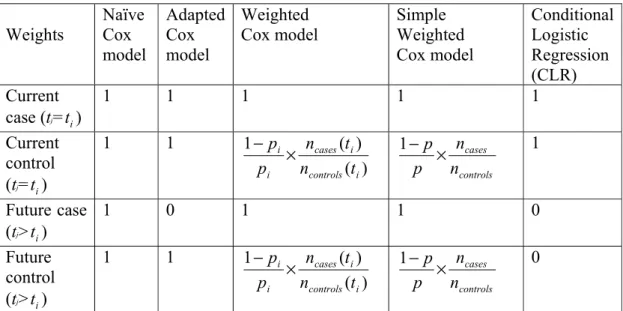
The details of definitions of weights in risk sets of Cox models are summarized in Table II.

Table II: definitions of weights in risk sets of models used for subject j at risk at aget_i : Weights Naïve Cox model Adapted Cox model Weighted Cox model Simple Weighted Cox model Conditional Logistic Regression (CLR) Current case (tj=t ) _i 1 1 1 1 1 Current control (tj=t ) _i 1 1 ) ( ) ( 1 i controls i cases i i t n t n p p × − 1 controls cases n n p p × − 1 Future case (tj>t ) _i 1 0 1 1 0 Future control (tj>t ) _i 1 1 ) ( ) ( 1 i controls i cases i i t n t n p p × − 1 controls cases n n p p × − 0

p: the life time probability of developing the disease of interest in the source

population.

i

p : the age-conditional probability of developing the disease of interest at age t or at _i

All the weighted Cox models were implemented by using the coxph function in the R statistical software. This function can directly handle such weights and relies on the robust sandwich variance estimator proposed by Binder [23].

4.2 Simulation study

4.2.1 Overview

To assess the performance of the Cox model with the new risk sets definitions, we carried out a series of simulations. First a hypothetical population was generated, and then a case-control study within that population was simulated. Several scenarios were investigated, and for each scenario the generating of population and case-control data was repeated 1000 times. The coding of the simulations was elaborated by Willy Wynant, who was Dr. Leffondré’s research assistant.

4.2.2 Generation of the source population

Source populations of size N=1000 subjects were generated. For each subject, several covariates were generated based on the empirical distributions of smoking variables observed in our real data. These data came from a large population-based case-control study of lung cancer undertaken in Montréal, Quebec, Canada, in 1996-2001 (for details see section 4.3.1). In all our simulation scenarios, all subjects were currently exposed at failure (i.e. diagnosis in real data) or censoring and we focussed our attention to three aspects of exposure: the cumulative value of exposure, the intensity and the duration of exposure. Note that the first aspect of exposure is a combination of the two others. We did not generate any non-time dependent exposure in our

simulation study since logistic regression performs well for estimating the effect of such exposures [7].

1. The age at exposure initiation, Aj, j=1,…,N, was generated from lognormal

distribution such that the age at exposure initiation had a mean _{μ = log(16.1)} and a standard deviation _{σ = log(4.1).}

2. The intensity at exposure initation, X0j, j=1,…,N , was generated from lognormal

distribution such that the intensity initiation had a mean _{μ = log(37.5) and a} standard deviation _{σ = log(20.0).}

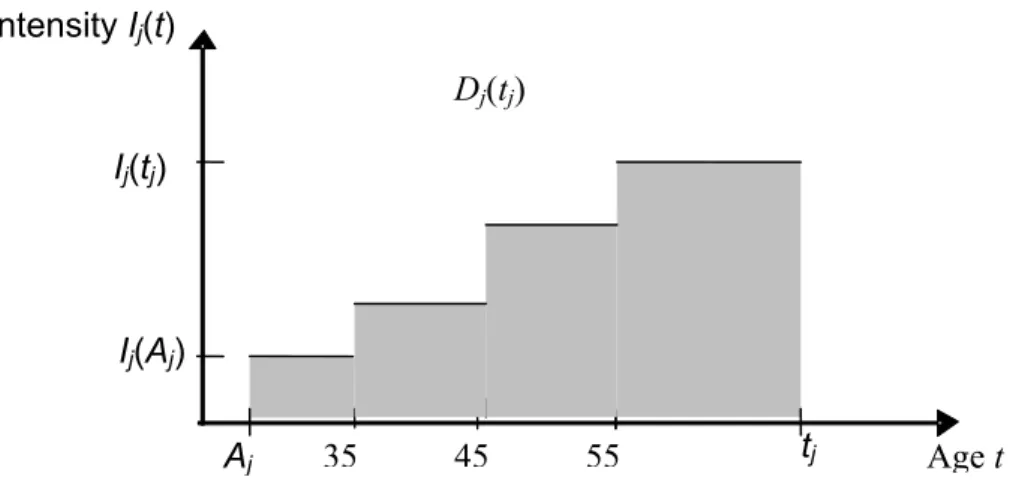
3. To reflect our real data on smoking intensity, where all subjects were asked to report their average number of cigarettes smoked per day at age 25, 40, 50, and 60 years, we generated an intensity of exposure according to a step function with predefined age intervals, as illustrated in Figure 2.

Figure 2 : Exposure pattern of a hypothetical subject j diagnosed or selected at age tj, with an

increasing intensity over lifetime. The value of the cumulative intensity at age tj, Ej(tj), equals to

the gray area under the curve. Where Aj is the smoking initial age, Ij(Aj) is smoking intensity at

the initial age, Ij(tj) is the intensity at age tj, Dj(tj) is the smoking duration at age tj which is equal

to tj minus Aj. Age t Ij(tj) Dj(tj) Aj 35 45 55 Ij(Aj) Intensity Ij(t) tj

Therefore, we assumed that the intensity of exposure was a monotone increasing or decreasing step function. Thus, we first generated a discrete variable to define the pattern of intensity over time: constant, increasing, or decreasing intensity, with probabilitiesq₁ , q₂ , or q , respectively. These 3 percentages varied depending on the scenario. Then, we assumed that the rate of increase or decrease at each step was constant over time within subject. For each subject j, its rate _τj of increase or decrease was generated from a

lognormal distribution with mean _{μ=0.4 and standard deviation σ=0.085 for} increasing intensity, and mean _{μ=0.1 and standard deviation σ =0.075 for} decreasing intensity.

4. Use a permutational algorithm to assign each subject j defined by the set of variables (X0j, Aj, τj) a survival time ti. See details below.

Permutational algorithm to generate survival times conditional on

time dependent covariates

To generate survival time conditional on time-dependent covariates, we used a permutational algorithm, which was first proposed by Abrahamowicz [21] and validated by MacKenzie [22]. Our algorithm consisted of the following steps:

• Simulation of survival times Ti*, i=1,…,N, assuming Gompertz distribution with

mean _{μ = 67.1 and standard deviation σ = 6.0.}

• Right censoring time Ci, i=1,…,N, was generated from uniform distribution

U[35,upper], where upper was defined so that 10% of survival ages Ti* were

• Sort the N tuples (ti, δi), where δi = I{ Ti*≤ Ci} is the indicator of

non-censoring and t_i = min(Ti*,Ci) is the survival time.

• Create the vector of current covariates values Xj(t ) for each subject j at each i

failure time t , i.e. past duration D_i j(t ), current intensity Ii j(t ) and cumulative i

exposure Ej(t ), as illustrated in Figure 2. i

• Randomly pair the vector of current covariates values Xj(t ) and (_i t , _i δ_i)

(j=1,…,N; i=1,…,N), according to probabilities based on the partial likelihood, from the earliest observed time t to the last time. If _{i δ}i = 1, then

randomly select an individual from the risk set R(t_i), with probability equal to his/her contribution to the partial likelihood at that time t . The subject who _i

will be selected in such a way will then be considered as the subject who fails at that time. Otherwise, if _δi = 0 and the censoring is independent of covariates

(as we assume here), then select an individual by simple random sampling from the risk setR(t_i). This subject will then be considered as the subject who is censored at that time.

4.2.3 Simulation of case-control studies

In each generated source population, we simulated a hypothetical population-based case-control study that was 1:1 age-matched case-control study. The cases were all the subjects who had event in the source population. Since we generated source populations of 1000 subjects, and that in average about 10% of these subjects had an

event, each case-control dataset was made of about 100 cases. For each case, a single control among subjects who were still at risk at the age of case’s event was randomly selected. This resulted in about 100 cases and 100 controls in each case-control data set. The set of potential controls for a given case included all future cases and controls, as well as past controls provided they were still at risk at the age of case’s event. Thus, if a subject was selected as a control, for example at age of 45 years, he could also be selected as a control again, e.g. at age 50, and had an event at age 55, for example. However in this case, in order to consider these subjects as different subjects, they were assigned a distinct ID number.

4.2.4 Summary of the different scenarios investigated

Several different scenarios were considered, each based on the proportional hazards model for the true effects of covariates on the hazard. With respect to exposure, we focus on distinguishing the effects of two aspects of exposure which may make distinct etiologic contributions: intensity and duration of exposure. In model 1 (see Table III), the hazard depended on current intensity and past duration, which were represented by two separate covariates. The distribution of the patterns of change in intensity over time varied across scenarios: in scenario 1, all subjects had decreasing intensity over time (q₁= 0%, q₂=0%,and q = 100%); in scenario 2, all subjects had ₃

increasing intensity over time (q = 0%, ₁ q =₂ 100%,and q = 0%); and in scenarios 3, 3 60% of the subjects had constant intensity, 25% had increasing intensity, and 15% had decreasing intensity over time (q₁= 60%, q₂= 25%,and q = 15%). For the 3

effects of intensity (βI) and duration (βD) on the hazard, we assumed βI = 0.02 and βD

= 0.05 or βI = 0.03 and βD = 0.08 in each scenario.

Table III : Summary of simulation scenarios in Model 1, hazard depended on intensity and past duration separately.

Intensity patterns of subjects¶ (%) True effect β Scenario No 1 q q₂ q₃ Intensity βI Duration βD 1 0 0 100 0.02 0.03 0.05 0.08 2 0 100 0 0.02 0.03 0.05 0.08 3 60 25 15 0.02 0.03 0.05 0.08

¶ q₁, q₂ and q₃ are the proportions of subjects who have a constant, increasing and decreasing intensity over lifetime in the source population.

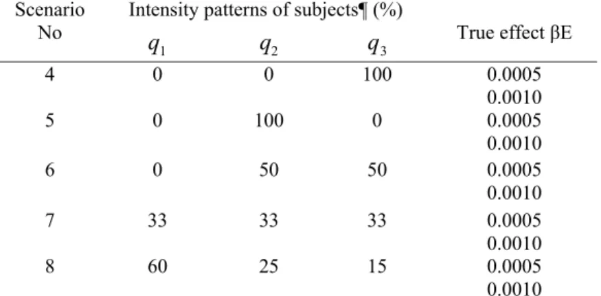
In Model 2 (scenarios 4-8, see Table IV), the hazard depended on the value of cumulative exposure, which was calculated as the area under the curve of intensity over time (see Figure 2). As in scenarios 1-3 for Model 1, the distribution of the patterns of change in intensity over time (q , ₁ q ,₂ and q ) varied across scenarios 4-8, ₃

and the true effect (βE) was equal to 0.005 or 0.010.

Table IV: Summary of simulation scenarios for Model 2, where the hazard depended on the value cumulative exposure*.

Intensity patterns of subjects¶ (%) Scenario

No

1

q q₂ q₃ True effect βE 4 0 0 100 0.0005 0.0010 5 0 100 0 0.0005 0.0010 6 0 50 50 0.0005 0.0010 7 33 33 33 0.0005 0.0010 8 60 25 15 0.0005 0.0010

¶ q₁, q₂ and q₃ are the proportions of subjects who have a constant, increasing and decreasing intensity over lifetime in the course population.

* Cumulative exposure was calculated as the area under the curve of intensity over time, as illustrated in Figure 2.

4.2.5 Data analytical models Logistic regression models

For the aim of comparison, logistic regression was used since it is the conventional method for case-control studies. Because individual matching was used in the simulation study, matched-pair analysis (e.g., conditional logistic regression) was used, and the matching variable itself cannot be analysed, e.g. age. As illustrated in the last column of Table II in the section 4.1, a standard conditional logistic regression procedure can be equivalent to a weighted Cox model, in which a weight of one is assigned to the two subjects (case and its control) at t , while a weight of i

zero is assigned to the rest subjects.

Existing Cox models

The two existing Cox models, i.e. the naïve version and the adapted version (See section 2.3.4 and Table II) were used in the simulation study, for the aim of comparison.

New proposed weighted Cox models

Since the source population was known in this simulation context, the weights of the risk sets of the two new models introduced in Section 4.1 were estimated from the generated population data. The age-conditional probabilities p were the proportions _i

of cases who had the events at age t or at a later age t > i t in the source population; i

and the lifetime probability p was the proportion of cases in the source population. Since it was a 1:1 age-matched case-control study, the ratio ncases / ncontrols was

systematically equal to one. Similarly, the case-control ratio in each risk set at any age t , _i n_cases(t_i)/n_controls(t_i), was systematically equal to one. Thus, the weights in equations (4.3) and (4.4) become:

⎪ ⎩ ⎪ ⎨ ⎧ ≥ − ≥ = i i i i i j t j p p t j t j j t age at control a as selected was subject the if 1 t age at failed case a was subject the if 1 ) ( ω (4.5) and ⎪ ⎩ ⎪ ⎨ ⎧ ≥ − ≥ = i i i j t j p p t j t j j t age at control a as selected was subject the if 1 t age at failed case a was subject the if 1 ) ( ω (4.6) Since the ages at event were precise enough in the simulation study, there were no ties among the survival times to handle in all the Cox models.

4.2.6 Summary statistics to evaluate the performance of the different analytical models

As mentioned in Section 4.2.1, all the scenarios were repeated 1000 times. The mean

βˆ of the 1000 estimated regression coefficientsβˆ , which is the log hazard ratio for

Cox’s models and the log odds ratio for logistic models, and the relative bias

β β βˆ )/

( ₋ were calculated for each scenario investigated. The ratio between the mean of the 1000 standard errors (SE) and the empirical standard deviation (SD) of the 1000 estimates was calculated to assess the accuracy of the variance estimators.

The coverage rate of the 95% confidence interval (CI) of the estimates,_βˆ± 961. ×SE, was calculated. The power of the Wald test was also calculated.

4.3 Real data analysis:

4.3.1 Data source

Study design

The real data that I used to investigate the performance of the new versions of the Cox models came from a large population-based case-control study of lung cancer undertaken in Montréal, Quebec, Canada, 1996-2001. The objective of this case-control study was to investigate the association between lung cancer and environmental and occupational exposures. It included both males and females, aged 35-75. Controls were frequency matched to cases on sex and age [24]. For the present analysis, our exposure of interest is smoking history, which was represented by different variables as explained below.

Smoking information

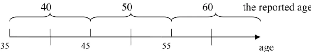
The information on smoking history available in the real case-control data are described in Table V. Each smoker was required to report average number of cigarettes smoked per day in average in the whole smoking period, and also at aged 25, 40, 50, and 60 years. To investigate the effect of smoking history in the Cox’s models, I assumed that those smoking intensities were constant around these ages 25, 40, 50, and 60 years. The smoking intensity was then represented as a time-dependent variable. For example: the average number of cigarettes smoked per day reported for

aged 40 represented the intensity from ages 35 to 45, the average number of cigarettes smoked per day reported for aged 50 was used to represent the intensity from ages 45 to 55, and the reported smoking intensity for aged 60 was used for the intensity after ages 55, as illustrated in Figure 3. Since this case-control study only included subjects aged from 35 to 75, the intensity at aged 25 was never used.

Table V: Summary of smoking variables in the case-control study, Montréal, Quebec, Canada, 1996-2001.

Variable name Type of variable

Smoking status Categorical (never smoker,

current smoker, ex-smoker)

Age at initiation continue (years)

Total duration continue (years)

Time since cessation continue (years)

Average number of cigarettes smoked per day over lifetime Average number of cigarettes smoked per day at age 25 Average number of cigarettes smoked per day at age 40 Average number of cigarettes smoked per day at age 50 Average number of cigarettes smoked per day at age 60

continue (cig/day)

Figure 3: The intensity at different age represented by the intensity at the reported age.

4.3.2 Method to handle missing smoking data

In all the analyses, I removed the subjects who were smokers but had not reported the average amount smoked cigarettes per day (11 subjects out off total 2190 subjects).

40 50 60

35 45 55 _age

Therefore, all smokers had the average smoking intensity over lifetime in the dataset of my analysis, however not all smokers had all intensities at the four reported ages. I did some imputation to handle these missing data. The method of imputation is described below.

One reason of the missing data is that some subjects started smoking later, or stopped smoking earlier than some reported ages. For example, if a subject started smoking at age 30, and quitted smoking (or was diagnosed with lung cancer) at age 55, he did not have reported intensities at age 25 and 60. Since in such a situation, the ages with missing value were out off the smoking period of that subject, the missing data did not influence the analyses when I represented intensity as a time dependent variable in the Cox models.

However, the situation was different if the missing intensity was inside the smoking period. For example, if a subject started smoking at age 30, and was diagnosed/interviewed at age 59, then the subject reported the average number of cigarettes smoked per day only at age 40 and 50. Since these two average numbers of cigarettes smoked per day can only represent the smoking intensity from age 35 to 55, there was a gap of the intensity from age 55 to 59. This kind of missing intensity at some age was caused by the definition of the range around each reported age, and could not be considered as missing at random.

To handle this kind of missing data, I used the intensity reported at the closest earlier age to represent the missing intensity at the later age, as illustrated in Figure 4, where

the intensity from age 55 to 59 was presented by the intensity at age 50. If no intensity was reported at a younger age, the average number of cigarettes smoked per day during the whole smoking period was used.

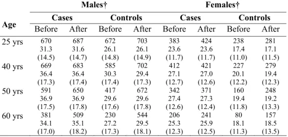
Table VI: Comparison of the distribution of smoking intensities (n, mean, standard deviation) before and after imputation to handle missing smoking intensity at each of the four ages (25, 40, 50, 60 years) in the case-control study, Montréal, Quebec, Canada, 1996-2001.

Males† Females†

Cases Controls Cases Controls

Age _{Before After Before After Before After Before After}

25 yrs 670 31.3 (14.5) 687 31.6 (14.7) 672 26.1 (14.8) 703 26.1 (14.9) 383 23.6 (11.7) 424 23.6 (11.7) 238 17.4 (11.0) 281 17.1 (11.5) 40 yrs 669 36.4 (17.3) 683 36.4 (17.4) 585 30.3 (17.4) 702 29.4 (17.3) 412 27.1 (12.7) 421 27.0 (12.6) 227 20.1 (12.2) 279 19.4 (12.3) 50 yrs 591 36.9 (17.5) 650 36.9 (17.8) 417 29.6 (17.6) 672 29.6 (17.8) 342 27.4 (12.6) 371 27.3 (12.4) 160 19.4 (11.8) 248 19.2 (13.3) 60 yrs 381 34.1 (17.0) 509 35.1 (18.2) 230 27.2 (17.3) 544 29.5 (18.1) 206 25.3 (12.3) 241 25.9 (12.5) 80 18.1 (11.3) 157 18.5 (13.5) † Among current and ex-smokers.

Figure 4: make up of the intensity at some age with missing data

The impact of the imputation on the distribution of the four reported smoking intensities is illustrated in Table VI. The data shown in this table suggest that the

40 50

35 45 55 _age

reported age

59