HAL Id: hal-02150163
https://hal.archives-ouvertes.fr/hal-02150163
Submitted on 21 Oct 2019
HAL is a multi-disciplinary open access
archive for the deposit and dissemination of
sci-entific research documents, whether they are
pub-lished or not. The documents may come from
teaching and research institutions in France or
abroad, or from public or private research centers.
L’archive ouverte pluridisciplinaire HAL, est
destinée au dépôt et à la diffusion de documents
scientifiques de niveau recherche, publiés ou non,
émanant des établissements d’enseignement et de
recherche français ou étrangers, des laboratoires
publics ou privés.
Distributed under a Creative Commons Attribution| 4.0 International License
An efficient strategy for large scale 3D simulation of
heterogeneous materials to predict effective thermal
conductivity
Xiaodong Liu, Julien Réthoré, Marie-Christine Baietto, Philippe Sainsot,
Antonius Adrianus Lubrecht
To cite this version:
Xiaodong Liu, Julien Réthoré, Marie-Christine Baietto, Philippe Sainsot, Antonius Adrianus
Lu-brecht. An efficient strategy for large scale 3D simulation of heterogeneous materials to predict
effective thermal conductivity. Computational Materials Science, Elsevier, 2019, 166, pp.265-275.
�10.1016/j.commatsci.2019.05.004�. �hal-02150163�
An
efficient strategy for large scale 3D simulation of heterogeneous
materials
to predict effective thermal conductivity
Xiaodong Liu
a, Julien Réthoré
a,⁎, Marie-Christine Baietto
b, Philippe Sainsot
b, Antonius Adrianus Lubrecht
ba Research Institute in Civil Engineering and Mechanics (GeM), CNRS UMR 6183, École Centrale de Nantes, 1 rue de la Noë, 44321 Nantes Cedex 3, France b Univ Lyon, INSA-Lyon, CNRS UMR5259, LaMCoS, F-69621, France
The behavior of heterogeneous materials (e.g. composite, polycrystalline) is one of the most challenging subjects for researchers. Imaging techniques based on X-ray tomography permit one to obtain the inner structure of these materials. To account for such detailed information and understand the material behavior, the use of tomo-graphic images as an input for numerical simulations is becoming more and more common. The main difficulty is the computational cost, mesh generation in the context of finite element simulations and the large discontinuities of the material properties, which can lead to divergence. The subject of this paper is to resolve these problems and understand the behavior of a material with high heterogeneity. The application of a MultiGrid method coupled with homogenization technique is proposed. The MultiGrid method is a well known method to increase convergence speed. The homogenization technique is applied to compute the coarse grid operators of the MultiGrid process. The combination of the two methods can efficiently deal with large property variations. Hybrid MPI/OpenMP parallel computing is used to save computational time. The influence of material het-erogeneity is analyzed as well as the ratio of material properties for the thermal conduction. The effective thermal conductivity of material is illustrated.
1. Introduction
The use of composite materials in many industrial fields has become more and more wide spread during the last decade. It is well known that many composite materials exhibit an excellent mechanical beha-vior. However, due to the complex structures and variable components of composite materials, it is not simple to understand their properties, which limits the application of these materials. Traditional experiments permit to globally characterize some of their properties. Nevertheless, it can just reduce this problem but not solve it fully. The characterization of the thermal properties of a composite material is an example.
Homogenization techniques have been developed to obtain effective thermal and mechanical properties of heterogeneous materials
[8,26,14]. The limitation of this method is that except for periodic materials, for which (under periodic boundary conditions) the predic-tion is robust, only upper and lower bounds of the effective properties can be obtained. For instance, for materials with high heterogeneity or with an irregular structure, this method has a poor performance. More importantly, the manufacturing process can neither ensure a defect-free material nor an exact geometry of the phases e.g. cast iron. In addition,
many materials, e.g. polycrystalline materials, have an intricate struc-ture. To sum up, one needs the real inner structure of the material to understand its behavior.
Fortunately, imaging techniques based on X-ray tomography show the inner structure of materials[13]. With these details, one can better understand the material behavior. Motivated by the secret of the ma-terial behavior, e.g. mechanical and thermal properties, using real to-mographic images as an input to perform numerical simulations is under development. Much work has been devoted to this subject. The work of Lengsfeld et al.[19]and Bessho et al.[2]presented the nu-merical simulation of bone tomography. They studied mechanical problems e.g. hip fractures of the human femur, using Finite Element Methods (FEM). Ferrant et al. [11], Michailidis et al. [20] and Proudhon et al. [23] also applied FEM simulations to tomographic images of industrial materials to analyze their properties. As we saw previously, FEM is widely used for this kind of simulations. Never-theless, the mesh generation of FEM needs human intervention, which is time consuming. The work of Gu et al.[15]that introduced a 3D simulation of the elastic behavior of a laminated composite material, proposed to use a Finite Difference Method (FDM), to take one voxel per
⁎Corresponding author.
E-mail address:[email protected](J. Réthoré).
grid to avoid heavy human work in the meshing step, and to use the MultiGrid (MG) method to accelerate the convergence speed. Besides numerical simulation, for instance, another choice to understand the material behavior, is to use tomographic techniques during the ex-periment. e.g. the work of[25]studied the heat conductivity for ma-terials with complex structures. However, to experimentally measure the heat conductivity of materials is still difficult, especially, for ma-terials with a complicated structure. e.g. composite mama-terials. It is still a challenge due to several kinds of problems e.g. thermal diffusion, thermal expansion during the experiment, material anisotropy.
Motivated by these practical considerations, the development of a standard process to obtain the effective thermal conductivity of het-erogeneous materials received considerable attention. This work takes the tomographic image as an input to a thermal conduction simulation to study the material thermal behavior and to obtain its effective con-ductivity.
The remainder of this paper is organized as follows. Section2 re-views the background, equations and some fundamentals of FEM. Section3presents the strategy for an efficient large scale simulation; Matrix Free FEM, MG method, homogenization techniques and parallel computing are illustrated in this section. Applications and results of this work are described in Section4. A discussion and conclusion section is provided in Section5.
2. Problem statement 2.1. Governing equations
Thermal conduction can be treated by a heat equation according to the first law of thermodynamics (i.e. conservation of energy):
∂ ∂ − ∇ ∇α = ρc T t ·( T) q̇ p v (1) where:
•
ρis mass density of material•
cpis specific heat capacity•
T is temperature•
t is time•
∇ denotes the gradient operator•
α is the thermal conduction coefficient which is a second order tensor•
q ̇v is the volumetric heat source.Since the focus of this work is thermal conductivity, it is considered that there is no extra source and the thermal field does not depend on time. The heat Eq.1becomes a typical Poisson equation:
∇ ∇·(α T)=div(α∇T)=0 (2) The tomographic images used in this study are cubicΩ∈ R3. Two
kinds of boundary conditions are applied on∂Ω as illustrated inFig. 1:
•
Dirichlet boundary condition (i.e. prescribed temperature) onΓ1andΓ2
•
Neumann boundary condition (i.e. prescribed heat flux) on the other four surfaces.which can be written as Eq.3: ⎧ ⎨ ⎩ = = ∇ = α T T T T T n 0 on Γ on Γ · on the other surfaces
0 1
1 2
(3) 2.2. Finite element discretization
FEM is one of the most common methods to discretize Ω and solve
the governing equations. However, the images representing the inner structure of the material have a very complex shape. The use of stan-dard meshes conforming to the phase geometry, requires much human work, as mentioned before and stated in the work of many researchers, e.g. Lengsfeld et al.[19], Bessho et al.[2], Ferrant et al.[11], Michai-lidis et al. [20], Proudhon et al. [23]and Nguyen et al. [21]. The strategy to use one node per voxel in the image has been chosen to avoid this difficulty. That means to assign the material property in each voxel on each elementary node. As the domain Ω is cubic and each voxel is cubic, 8-node cubic elements are chosen to discretize Ω.
Multiplying Eq.(2)with a test function and integrating over Ω, one obtains:
∫
div(− ∇α T φ d) Ω=0Ω (4)
whereφis the test function.
Applying integration by parts, the formula reads:
∫
∫
− ∂ α∇ →T n φ dS· + α∇ ∇T· φ dΩ=0
Ω Ω (5)
where− ∇ →α T n· is the heat flux in the outward normal direction→n on the boundary. Eq.5can be summarized as:
∫
∂ α∇ →T n φ dS· =∫
α∇ ∇T· φ dΩΩ Ω (6)
Employing finite element discretization, one gets:
∑
→≈→= = T Th T φ i N i i 1 (7)where→Th={ ,T T1 2,…, }Tn is an approximate solution of T N, denotes the number of unknowns and φi is the shape functions of 8-node cubic elements, which is the same as the test function.
Finally, Eq.(6)can be written as:
∫
∫
∑
∇ ∇ =∑
∇ → = = ∂ α α T φ· φ dΩ ( T φ n φ dS)· i N i i j i N i i j 1 Ω 1 Ω (8)After using Gauss integration on the integral above,αused in the FEM equation becomes the conductivity in each Gauss integration point
αg. It is obtained by the interpolation with shape functions, and, de-scribed as:
∑
= = αg α φ· s s s g 1 8 , (9) where s denotes the shape function assigned with each elementary node,φs g, the value of shape functions at Gauss integration points andαs elementary node conductivity.From Eq.(8), one obtains a system of equations: →=→
T f
L h (10)
whereLis a matrix which is often referred to as the stiffness matrix,→Th
is a vector containing all unknowns (temperature at each node) and→f
is the right hand side vector.
The aim is to solve Eq.(10)to obtain the unknownsTi.
3. Implementation 3.1. Iterative solution
The best known solution algorithms for Eq.(10)are direct solvers and iterative solvers. For the direct solver, one has to assemble the stiffness matrix, which requires a large memory. The largest image that will be computed in this application is an image containing
× ×
2049 2049 2049voxels, which means that the number of elements is 20483(i.e. more than eight billion elements). Supposing one uses cubic
elements with 8 Gauss integration points, the size of global sparse matrix is2049×2049×2049×27×8bytes≈1.69TB. It is impossible to have such a huge memory space available on a normal computer. The size of the stiffness matrix does not allow one to assemble the whole matrix. It forces one to use an iterative solver without assembling the stiffness matrix, which is often called the Matrix Free Finite Element Method (MF-FEM). The work of Carey and Jiang[7]invented MF-FEM. For instance, this method is developed and widely used, especially, for parallel computing (see e.g. Tezduyar et al.[28]). Flaig and Arbenz[12]
also developed a matrix-free MultiGrid solver for tomographic image simulation. In this work, one proposes to use a MF-FEM with the di-agonal value of the stiffness matrix to accelerate the convergence rate. 3.2. MultiGrid and homogenization
The iterative single level Jacobi solver applied previously can quickly decrease the high frequency components of the error, but for low frequency errors, it does a poor job. The convergence speed di-minishes rapidly as presented inFig. 5a.
It is well know that the MG method is one of the most efficient ways to increase the convergence rate. The idea of MG is to construct several levels or grids. Then, iterative relaxations are carried out at each level, high-frequency errors can be eliminated on fine grids and low-fre-quency errors can be eliminated on coarse grids (e.g. work of[5,6]). With this method, one can solve the slowness problem of single level Jacobi relaxation due to the presence of low-frequency errors. The work of Biboulet et al.[3]shows the efficiency of using a MG method on the FEM. However, they assembled the stiffness matrix which, is very ex-pensive for large scale problems.
Nevertheless, a standard MG method is not adapted for problems with high heterogeneity. It has a very poor convergence performance, when large variations of the material properties are to be considered, or rather, high temperature gradients on coarse grids are involved. These variations make the linear prolongation and restriction operators al-most ineffective. However, the material property on a coarse grid is unknown and it is should be chosen to avoid the poor performance of classical coarse grid and inter-grid operators.
To resolve these problems, one needs new coarse grid operators, prolongation operators and restriction operators. Several researchers have investigated this problem, such as the work of Alcouffe et al.[1]
for 2D, Hoekema et al.[17]for 3D, Engquist and Luo[9]and Engquist and Luo[10]. These researchers proposed several methods to alleviate the poor convergence of the standard MG method. But the problem is that the implementation of these ideas is not simple. The computational time and memory cost are the two other limitations. Based on the work of Alcouffe et al.[1]and Sviercoski et al.[27], some new operators for the MG method are proposed in this paper.
Sviercoski et al.[27]proposed to use a Cardwell and Parsons (CP) bounds type homogenization to get the analytical coarse grid operator. The idea is to compute the upper and lower CP bounds of the material property on each coarse grid from the finest grid. After that, the average
of the arithmetic and geometric averages of the CP bounds, is supposed to be the effective property on each coarse grid. With this strategy, one can obtain the diagonal components of the material property tensor, which is already sufficient for isotropic materials. For anisotropic ma-terials, they proposed a method to calculate the off-diagonal compo-nents of the property tensor. With the effective material property tensor, the coarse grid operator on each level can be easily obtained by the equation below:
∫
= ∇ α ∇ LH ϕi ¯ ϕ dΩ H H j H Ω (11) where,ϕiH and ϕ jH are test functions on each coarse grid,α¯H is the effective material property tensor of coarse grid.
The weak point of Sviercoski et al.[27]is that, the CP bounds on each coarse gird has to be computed from the finest grid. It requires too much computational time when using many grids. Therefore, one proposes to use different homogenization bounds which can be com-puted level by level.
Among different homogenization methods, the Voigt approximation is one of the best-known methods. In addition, it can be computed re-cursively. It is also referred to as the arithmetic mean:
∑
= = = α α N xxHV k k N xxh h 1 h (12) whereαxxHV is the diagonal component ofαHV which is the average obtained by Voigt homogenization on coarse gridl−1,αxxh is the di-agonal component of αhwhich is the material property on the fine grid l,x=1, 2, 3,Nhis the number of nodes on level l, which has the same volume as one element on levell−1.Another approximation often used is the Reuss approximation. Equally, it can be obtained recursively, It is also known as the harmonic mean:
∑
= = = − α N α xxHR h k k N xx h 1 1 h (13) whereαxxHRis the diagonal component ofαHRwhich is the average ob-tained by Reuss homogenization at the gridl−1.Instead of the CP bounds, the Voigt-Reuss (VR) bounds are used in this work. Thus the effective material property tensor can be obtained recursively. The assumption is that the effective value lies within the arithmetic and geometric averages of the VR bounds.
Definition: The effective material property tensorα¯His the average of the arithmetic and the geometric average of the VR bounds. Which is presented as:
= +
α 1 α α
2( )
xxH xxa xxg (14)
where,αxxHis the diagonal component of α¯ ,H αxxa is the diagonal value of the arithmetic average of the VR bounds which is defined as:
= +
αxxa (αxxHR αxxHV),αxxg
1
2 is the diagonal value of the geometric average
of the VR bounds which, is defined as:αxxg = αxxHR·αxxHV.
The material used in this work is supposed to be isotropic, off-di-agonal values ofα¯H are zero. The strategy to obtain the off-diagonal components is therefore not presented in this work.
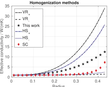
An analysis of different homogenization methods (e.g. Voigt, Reuss, Hashin-Shtrikman, Self-Consistent) has been performed, to confirm the strategy used in this work. The idea is to compute the effective thermal conductivity for a cubic structure, in which there is a spherical inclu-sion.
•
The conductivity of the sphere is 100 W·m ·−1K−1, 1 W·m ·−1K−1for theother part of the cube
•
The radius of the sphere is between 0 m and 0.4 mFig. 2 illustrates the evaluation of the effective conductivity ob-tained by different homogenization methods, when the sphere radius varies. The effective property obtained by the VR bounds lies between the Hashin–Shtrikman bounds. It confirms that the method used in this work is robust and efficient.
Besides the coarse grid operators, prolongation and restriction op-erators also need special treatment. The relation between the restriction operators (i.e.R) and the prolongation operators (i.e.P) is:
=
P RT (15)
The work of Boffy and Venner[4]presents the principle to derive P and R. The point is to consider the material discontinuities. The prolonga-tion process will be briefly presented in this paper.
As illustrated inFig. 3, the big box with solid edges represents one element on the coarse gridl−1, and, the eight small boxes with dotted edges are the eight elements on the fine grid l. The temperature at each “black” node (e.g.A1,A2) of coarse grid is known. The goal is to obtain the temperature at all the 27 nodes of the fine grid. For the temperature at the eight “black” nodes of the fine grid coinciding with the ones on the coarse grid, one does an injection, which means:
= −
TAl1 TAl11 (16)
For the other nodes, instead of the linear prolongation of the stan-dard MG method, the nodal material property is taken into account. It
reads as follows.
For the “red” nodes (Fig. 3) located at the center of the link between two coarse grid nodes (e.g. nodeB1):
= + + − − T α T α T α α Bl A A l A Al A A 1 1 1 1 2 21 1 2 (17)
For the “blue” nodes which, are located at the center of each face of the big box (e.g. node C1):
= + + + + + + T α T α T α T α T α α α α Cl B Bl B Bl B Bl B Bl B B B B 1 1 1 2 2 3 3 4 4 1 2 3 4 (18)
For the “yellow” center node of the big box (e.g. node O):
= + + + + + + + + + + T α T α T α T α T α T α T α α α α α α Ol C Cl C Cl C Cl C Cl C Cl C Cl C C C C C C 1 1 2 2 3 3 4 4 5 5 6 6 1 2 3 4 5 6 (19)
With this strategy, the material property at each node weighs its contribution for the prolongation. It is obvious that, ifαis constant, it becomes the linear prolongation of the standard MG method.
Finally, the application of the V-cycles MG method coupled with homogenization technique can be illustrated by the following steps:
1. Compute Voigt and Reuss approximations on each level, re-spectively; obtain the effective material propertiesα¯H for all le-vels besides the finest level which, has the real material proper-ties.
2. Carry out relaxations with the Jacobi solver on level l. 3. Transfer the temperature and restrict the residual to level −
l 1and perform relaxations on this level.
4. Repeat steps2, 3, 4from the finest grid to the coarsest grid =
l 1.
5. Prolong the correction to the levell+1and relax on this level.
6. Repeat step 5 until the finest level.
7. Loop step 2, 3, 4, 5, 6 until obtaining the required residual. 8. Output results.
To have a better performance, instead of using only V-Cycles, the full MultiGrid (FMG) cycles are used in this work. Comparing to one V-Cycle, one FMG cycle need more relaxations on coarse grids. However, the computational cost on coarse grid is negligible compared to fine grid. Further, FMG cycles provide for a good initialization solution on the finest level, the number of relaxations on the finest gird is thus lower than that of V-Cycles. The scheme of FMG cycles for 3 levels is illustrated inFig. 4. For all of the applications in this work, one starts always by a ×4 4×4grid on level 1. The size of grids for levell+1is two times smaller than that of level l, e.g. for a problem of 20483
ele-ments, one has 10 levels.ν0is the number of relaxations performed on
level 1,ν1is the number of relaxations performed on each level going
up.ν2is the number of relaxations performed on each level going down.
For this FMG cycles, one uses ncyV-Cycles on each level. For the initial solution of each fine level +l 1, one does a bi-linear interpolation of the solution of level l.
Fig. 2. Different homogenization methods.VR+: VR upper bound,VR−: VR lower bound, HS+: Hashin-Shtrikman upper bound,HS−: Hashin-Shtrikman lower bound, SC: Self-Consistent.
The performance of the MG scheme is studied below. One carries out a simulation of a spherical thermal inclusion with a conductivity of 10 W·m ·−1K−1for sphere and 1 W·m ·−1K−1for the other part of the cube.
The radius is a quarter of the size of cube. The domain Ω is discretized with 1283(more than two million) elements. The boundary conditions
are set according to Eq.3. The simulation is run on an office computer equipped with one processor “Intel(R) Core(TM)2 Quad CPU Q9650 @ 3.00 GHz”. For the single level iterative relaxation, the Jacobi relaxa-tion is applied directly on this 1283grid problem. For the MG scheme,
one has 6 level for this 1283grid problem, ν ν ν n, , ,
cy
0 1 2 are set to be 10,
1, 2 and 5, respectively. Three different values for the relaxation coefficient ω, i.e. 0.5, 1.0 and 1.5, are used for both simulations.
Table 1andFig. 5illustrate the performance of the MG scheme and the single level Jacobi solver. The convergence rate of the single level Jacobi solver decreased rapidly both for damped Jacobi withω=0.5 and normal Jacobi withω=1.0. On the other hand, the convergence rate of the MG scheme remains constant withω=0.5andω=1.0. For the case of over relaxation i.e.ω=1.5, it diverges with both methods for this problem. With a ω=1.0, one has the best convergence perfor-mance for the MG scheme. After 4139 relaxations, single level Jacobi relaxation does not yet reach the initial solution of FMG cycles on the finest level, it confirms that one can have a good initial solution for the finest level with FMG cycles. If one ignores the computational cost on coarse grids, the MG scheme costs about 276, i.e.4139
15 , times lower, with
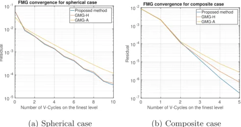
a residual 10 000 times smaller than that of single level Jacobi solver. Another study is also carried out to compare the convergence per-formance between classical MG and the proposed method. Compared to the classical Geometric MultiGrid (GMG), the proposed method has two differences:
•
Instead of the bi-linear prolongation and restriction operators, one proposes to consider material property for the prolongation and restriction operators.•
Homogenization technique is used in the proposed method to obtain the coarse grids material properties, however, in the classical GMG, a simple average, i.e. Voigt approximation, is often used for the coarse grids material properties.According to the difference between a classical GMG and the
proposed MG, one proposes to carry out three simulations for the spherical case with a material property contrast of 1 000 (detailed in Section4.2) and and the composite case (detailed insection 4.4).
•
GMG-A: Bi-linear restriction and prolongation operators, Voigt ap-proximation material property for coarse grids•
GMG-H: Bi-linear restriction and prolongation operators, homo-genized material property for coarse grids•
Proposed method: Considering material property for restriction and prolongation operators, homogenized material property for coarse gridsAs illustrated inFig. 6a and b, these three methods converge for both spherical and composite case. For spherical case, both the pro-posed method and GMG-H have the best performance. For the com-posite case, the proposed method has the best performance. For both cases, it shows that coarse grid material property has a large influence on the convergence speed, a representative material property for coarse grid is highly important to ensure good convergence. The idea to in-cludes the material property for the prolongation and restriction op-erators does not always have a large improvement, for some symme-trical case, e.g. spherical inclusion, it does not have a large improvement compared to GMG-H. But for the complex case e.g. com-posite material, it has a good performance. As the aim of the proposed algorithm is to deal with complex materials with large property varia-tions, the proposed algorithm is more efficient.
3.3. Parallel computing
As mentioned above, the goal of this work is the simulation of a domain discretized by more than eight billion elements, with a single processor, the computational time and memory are a big challenge.
These limitations lead one to consider High Performance Computing (HPC). The available machine is a supercomputer equipped with 252 nodes with 128 GB RAM for each node. Each node consists of two processors and each processor has 12 cores. Message Passing Interface (MPI) and OpenMP are the two most used methods for parallel com-puting. MPI is mainly for distributed memory machines, whereas, OpenMP is for machines with a shared memory. Using OpenMP only can not address our problem, as the memory of one node is not suffi-cient. MPI only can be a choice, but the difficulty is that, for the coarsest grid, one has only ×4 4×4elements. By consequence, for the coarsest level, one can uses only 64 MPI, which does not allow a good speedup (maximum 64). To take advantage of this machine, we uses a hybrid MPI/OpenMP parallel algorithm.
Table 1
Comparison between single level relaxation and a MG scheme.
Single level MG scheme Residual achieved 1.55×10⁻² 7.89×10⁻⁶
Number of relaxations on the finest level 4139 15
Fig. 5. Convergence of the Jacobi solver (a) and MG scheme (b) on a 1293nodes problem.
4. Results and applications 4.1. Validation
A multi-layer problem is used to validate the proposed solver. The domain Ω:1.0×1.0×1.0 cm3cube, consists of four uniform layers. The
thermal conductivity of each layer is:α1=1W·m ·−1K ,−1 α2=4W·m ·−1 −
K1,α =8
3 W·m ·−1K−1andα4=4 W·m ·−1K−1. The distribution of these
four materials is presented inFig. 7. Boundary conditions are applied as mentioned in Eq.3.T1=0K andT2=1K are applied.
The analytical solution of this problem can be described as:
= ⎧ ⎨ ⎪ ⎪ ⎩ ⎪ ⎪ ⩽ < + − ⩽ < + − ⩽ < + − ⩽ ⩽ T z z z z z z z z z ( ) for 0 0.25 cm ( 0.25) for 0.25 cm 0.5 cm ( 0.50) for 0.5 cm 0.75 cm ( 0.75) for 0.75 cm 1.0 cm 32 13 8 13 8 13 10 13 4 13 11 13 8 13 (20)
where z is the coordinate of axis Z.
To validate the numerical solution, the error between the analytical and the numerical solution is computed. However, the FEM has a dis-cretization error, the number of elements used to obtain the numerical solution affects the error between the analytical and the numerical solution. As a result, on one side, the error between the analytical and the numerical solution is analyzed; on the other side, the FEM dis-cretization error is studied.
For the numerical solution, one discretizes Ω into128×128×128 (i.e. more than two million) cubic elements, applies the same boundary conditions as for the analytical solution and carries out the simulation. The coarsest level has 4 × 4 × 4 grids, for each finer level, the grids size is devised by two i.e. 6 levels for a 1283problem.Fig. 8shows the
temperature variations of the analytical and the numerical solution, respectively, along the Z direction. The temperature obtained by the numerical simulation is almost the same as the one obtained by the analytical solution. TheL2error norm between the analytical solution
and the numerical solution is 0.0027.
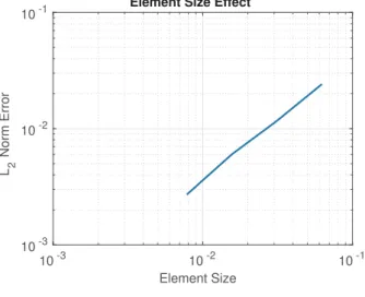
To analyze the influence of the element size, one discretizes Ω with × ×
16 16 16,32×32×32and64×64×64elements and computes the
L2error norm compared to the analytical solution, respectively.Fig. 9
shows the l2error norm as a function of element size. TheL2norm error
decreases almost linearly in log–log scale with the element size. The analytical and numerical solution show that the strategy of using the MG method coupled with homogenization technique can deal with problems with varying coefficients.
4.2. Spherical inclusion with large variation
The stability of the proposed method is analyzed in this subsection, when it handles a spherical inclusion problem with large material property variations. The parallel performance of our program is also studied for this application.
The domain Ω is a cube, which has two materials, as presented in
Fig. 6. Convergence of MG method with different intergrid operators.
Fig. 10a. The radius of the inclusion isR=L
4, where, L is the size of
cube. The thermal conductivity of the material in the sphere is 1 000 W·
−
m ·1K−1, whereas it is set to 1 W·m ·−1K−1in the other part. The contrast
between these two materials is 1 000. One discretizes the cube with
× ×
128 128 128cubic elements. The boundary conditions is presented in Eq.3. The coarsest starts always by a 4 × 4 × 4 grid. ν ν ν n0, 1, 2, cy are set to be 100, 4, 8 and 10, respectively.
Fig. 10b shows the temperature gradient in Ω. The large variation of
the conductivity on the interface explains the large variation of the temperature gradient around the interface.
This application confirms the good stability of this strategy in case of large variations of material properties.
4.3. Effective conductivity of cast iron
Cast iron is a well-known and widely used material in the industrial domain. The prediction of the conductivity of cast iron is a significant difficulty for researchers. Several papers investigate the conductivity, e.g. Helsing and Grimvall[16]regarded cast iron as a composite ma-terial and created a model to predict its conductivity. Nevertheless, since the distribution of carbon grains in cast iron affects its con-ductivity, the property of cast iron is different for different manu-facturers. One proposes to use X-ray tomographic techniques to obtain the carbon grains distribution in an image format. The numerical si-mulation is then employed on this image to analyze the influence of carbon granules and to obtain the effective conductivity of cast iron.
The original tomographic image of cast iron is an image with
× ×
512 340 340voxels[24]. The voxel size is 5.06μm. The region of interest (ROI) in this work is a part of this image. This part has
× ×
257 257 257(more than 16 million) voxels. Each voxel is supposed to be one elementary node of the FEM discretization. A conductivity is assigned to each node.Fig. 11a illustrates the conductivity of the two components in cast iron, where, the black granules in this image are the carbon grains. The carbon conductivity is 129.0 W·m ·−1K−1, for the
other part, one takes the conductivity of iron which, is 80.4 W·m ·−1K−1.
To obtain the effective conductivity of the cast iron, the homo-genization method is used. As presented in the work of Özdemir et al.
[22], the idea is to consider Ω to be one element, which is also referred to be a Representative Volume Element (RVE). The theory of RVE homogenization is briefly presented below.
The well known Fourier’s law is described as:
−A·∇ =θ Q (21)
where, A is the effective thermal conductivity at macroscopic scale, θ is temperature at macroscopic scale,∇θis its gradient and Q is the total heat flux at macroscopic scale, which can be computed from the local heat flux:
∫
∫
= = − α∇ Q V q dv V T dv 1 1 V V (22)Three simulations are carried out with: ⎧ ⎨ ⎪ ⎩ ⎪ ∇ = ∇ = ∇ = = ∇ ∂ ⎧ ⎨ ⎪ ⎩ ⎪ ∇ = ∇ = ∇ = = ∇ ∂ ⎧ ⎨ ⎪ ⎩ ⎪ ∇ = ∇ = ∇ = = ∇ ∂ − − − θ θ θ T θ x θ θ θ T θ y θ θ θ T θ z 1 K·m 0 0 on Ω 0 1 K·m 0 on Ω 0 0 1 K·m on Ω x y z x x y z y x y z z 1 1 1 (23)
Fig. 8. Temperature variation on Z direction of the analytical (Red) and the numerical (Blue) solution.
Fig. 9. L2norm error analysis.
Fig. 10. Spherical inclusion.
respectively, where∇θx,∇θyand∇θzare the temperature gradient in direction X, Y and Z, respectively. With each boundary condition, one column of A can be obtained.
For the FMG Cycles, 7 levels of grid are used, ν ν ν n0, 1, 2, cyare set to be 10, 2, 1 and 5, respectively.Fig. 11b shows the distribution of the temperature gradient in the case of∇ =θz 1, in which there are many inclusions. The location of the inclusions coincides with the location of the carbon grains.
The effective conductivity obtained is: = ⎧⎨ ⎩ − − ⎫ ⎬ ⎭ − − A 82.4311 0.0020 0.0040 0.0020 82.4223 0.0026 0.0040 0.0026 82.4277 W·m ·K1 1
Up to two significant digits, A can be described as: = ⎧⎨ ⎩ ⎫ ⎬ ⎭ − − A 82.43 0.00 0.00 0.00 82.42 0.00 0.00 0.00 82.43 W·m ·K1 1
which means that cast iron of this manufacturer is almost isotropic regardless of the random carbon distribution.
4.4. Effective conductivity of a layered composite material
Cast iron is almost isotropic, one may measure its conductivity ex-perimentally. However, for layered composite materials, which are also widely used in the industrial domain due to its good performance, can be an anisotropic material. To carry out an experimental measurement, several external factors have to be observed, which is not simple and sometimes, not possible. Employing numerical simulations directly on tomographic images can be good alternative to know the composite properties.
The image used in this work is the image of a laminate composite material consisting of unidirectional E-glass fibers and a M9 epoxy matrix. It is a Glass Fiber Reinforced Polymer (GFRP) manufactured by the Hexcel Company. Its mechanical properties have been studied by Lecomte-Grosbras et al.[18]. The details of this image can be found in the work of Lecomte-Grosbras et al.[18]. In this work, the heat transfer in this GFRP is studied to obtain its effective conductivity.
The original image of this GFRP is an image consisting of
× ×
700 1300 1700 voxels, As mentioned in the work of Lecomte-Grosbras et al.[18], this material is designed with four layers, the or-ientation of fibers is +15 ,° − ° − °15 , 15 and+15°, respectively, for each layer. The idea is to take a cubic domain from the part which has the same fiber orientation. One takes129×129×129voxels from the part with a fiber orientation of −15°, as the ROI (seeFig. 12). As presented in12, the interface between the E-glass fiber and M9 epoxy matrix is not extraordinarily sharp. It is difficult to distinguish between these two phases (matrix and fiber). Instead of applying two discontinuous phases, one proposes to apply a continuous conductivity between 0.150 W·m ·−1K−1 (epoxy) and 1.30 W·m ·−1K−1 (E-glass fiber). One
chooses to smooth the image gray level before it is used to compute the local material property at each voxel. It can be described as:
= ⎛ ⎝ − − − + ⎞⎠+ −
(
)
α 0.575 1 e |GL20160.5| sign GL( 160.5) 1 0.15 (24) where GL is the original value of each voxel obtain by X-Ray tomo-graphy, which is an integer between 0 and 255. Except for the problem of the allocation of the conductivity, another problem is that the dia-meter of fiber is too small to have enough voxels in it. Sub-sampling i.e. linear interpolation, is therefore applied to this ROI to have more voxels in each fiber. The FEM discretization error therefore needs to be ana-lyzed, to obtain the number of voxels needed for each section. A si-mulation with∇ =θz 1W·m ·−1K−1,∇ = ∇ =θx θy 0andT= ∇θ zz on∂Ω is performed. One time sub-sampling (case I) and two times sub-sampling (case II) are applied to the ROI, respectively. Fig. 13 illustrates the conductivity of each node in this ROI after one time sub-sampling. Forthe FMG Cycles, ν ν ν0, 1, 2, ncyare set to be 10, 2, 1 and 5, respectively. The third column of the effective property tensorAcis computed for
each case.
For case I (7 levels i.e.2573nodes):
= −
Ac3 { 0.001559 0.025400 0.744922} For case II (8 levels i.e.5133nodes):
= −
Ac3 { 0.001607 0.026223 0.745158}
It means that about up to three significant digits, the third column of the effective conductivity tensor is the same, or rather, one can take three significant digits for theAcobtained by one time sub-sampling,
which is sufficient for industrial applications. The temperature gradient is also computed, as presented inFigure 14.
Similar to the previous cast iron application, other two simulations with boundary conditions of Eq. (23) are performed. The effective
Fig. 12. ROI of the GFRP.
conductivity of the ROI of the GFRP is: = ⎧⎨ ⎩ − − ⎫ ⎬ ⎭ A 0.625386 0.002162 0.001559 0.002162 0.628834 0.025400 0.001559 0.025400 0.744922 W/(mK) c
With up to three significant digits, it reads: = ⎧ ⎨ ⎩ − − ⎫ ⎬ ⎭ A 0.625 0.002 0.002 0.002 0.629 0.025 0.002 0.025 0.745 W/(mK) c
which confirms that GFRP is an orthotropic material.
The effective property tensor obtained above, is for the fibers with an orientation of−15°, for that of the+15°orientation, one can derive it directly.
4.5. Large simulation from a X-ray tomographic image and HPC performance analysis
The applications introduced above reveal that, the effective con-ductivity can be obtained by numerical simulation directly from an X-ray tomographic image, without any human intervention. The current tomographic images have2048×2048×2048 voxels or more than 8 billion elements. The final application for this work it to carry out the numerical simulation with such a large image.
The image used in this case is the GFRP image of the previous ap-plication. One takes a part from the original image, the ROI consists of
× ×
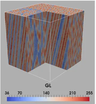
513 513 513voxels. As presented inFig. 15, it consists of four layers with different E–glass fiber orientations. One employs a two times sub-sampling to obtain an image consisting of2048×2048×2048elements. The smoothing process on gray level is also applied and the material property has been assigned to each node as presented inFig. 15. The same boundry conditions are applied as for the spherical inclusion case. For the FMG cycles in this simulation, 10 levels of grids are used,ν0,
ν ν n1, 2, cyare set to be 10, 2, 1 and 5, respectively. 768 cores (64 MPI, 12 OpenMP/MPI) are used simultaneously. The calculation time is about 3.16 h. Figure 16 illustrates the residual evolution with the number of V-Cycles on level 10. Regardless of the size of the problem, the convergence remains very good. To achieve a residual of10−6, only
5 V-Cycles on the finest level are needed. It means that the number of relaxations on the finest level is only 15. It confirms the efficiency of the
strategy used in this work. The temperature gradient is presented in
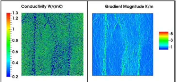
Fig. 17. Fig. 17 and 18 illustrate the correspondence between con-ductivity and temperature gradient.
Since the aim of this work is the computation from large tomo-graphic images, the parallel computing performance is analyzed with a
Fig. 14. Temperature gradient of E-glass fibers in composite.
Fig. 15. E-glass fiber orientation in each layer and conductivity at each ele-mentary node.
0 1 2 3 4 5
Number of V-Cycles on the finest level
10-6 10-5 10-4 10-3 10-2 10-1 Residual FMG convergence Fig. 16. Convergence.
problem of 10243elements. A one-time sub-sampling is applied on the
5123ROI to obtain an image of 10243elements. The aim is to analyze
the parallel performance, so, instead of doing FMG cycles until final convergence, one proposes to do only one V-cycle on the finest grid.
For the performance of hybrid programming, there are two para-meters to investigate: the number of MPI used and the number of threads per MPI task. As mentioned before, each processor has 12 cores for the available machine, each node has 2 processors. In order to have a good efficiency, the number of threads per MPI is limited by 12 to avoid the use OpenMP between two sockets, since OpenMP suffers from poor data access patterns when using two sockets. The number of cores maximum that can be used is 1 000 fixed by the owner.
As presented inFig. 19, one simulation with 1 core and 1 MPI has been carried out to have a reference to compute the speedup. The number of MPI is set to 1,2,4,8,16,32 and 64; 12 threads are used in each MPI task. This curve illustrates that for a 10243 problem, even
with 768 cores, good speedup is obtained, within this number of cores, the speedup increases linearly as the number of cores increasing. Fur-ther, the speedup is close to be optimal, the speedup rate being close to 0.8.
Besides the number of cores that has a big influence on the parallel performance, the number of MPI and the number of OpenMP (for the same number of cores) can also have an influence: i.e. for 384 cores, one has the following configurations: 32 MPI with 12 threads, 48 MPI with
8 threads, 64 MPI with 6 threads, 96 MPI with 4 threads, 128 MPI with 2 threads.
Simulations for three different configurations, i.e. 32 MPI with 12 threads, 48 MPI with 8 threads and 64 MPI with 6 threads, are carried out for a problem for 10243elements. As presented inTable 2, with 48
MPI and 8 threads per MPI, one has a poor performance since in one node, there are 3 MPI which means there is at least one MPI taking cores from two sockets. With 64 MPI and 6 threads per MPI, one obtains a better performance than that with 32 MPI and 12 threads for each, but the difference is only480−463≈3.67%
463 . It confirms that nevertheless the
current program does not allow to use as more as MPI tasks that we want, but with 64 MPI and 12 cores, a sufficient performance is ob-tained. For some large problems likes 20243grids, using 12 cores for
each of the 64 MPI, i.e. 768 cores in total, one can already finish the simulation in about 3 h.
5. Discussion and conclusions
The goal of this paper is to show that one can employ numerical simulations directly on tomographic images. To perform the simula-tions with such a large number of elements and such large variasimula-tions of materials properties requires dedicated algorithms and hardware. The strategy to use the MG method coupled with a homogenization tech-nique, permits one to deal with this kind of problems. The applications and numerical comparison presented above demonstrate the efficiency of the MG method. The homogenization technique shows its capacity to increase the convergence performance of the MG scheme, when large variations of materials properties exits. The Matrix Free FEM demon-strate its good performance for large problems up to 8 billion of ele-ments. The strategy to apply one voxel per elementary node avoids human intervention. The effective material property can be auto-matically obtained by using the large X-ray tomographic image, as an input, without complex experimental measurement. The Hybrid MPI/ OpenMP programming shows its good feasibility and performance for the MG method.
The thermal conductivity is analyzed in this work. In future work, the mechanical property of materials will be analyzed. The property at each node is supposed to be isotropic, additional research is needed for the anisotropic case. For the parallel computing of MG method, the re-partitioning and load balancing need to be applied for the future work if necessary to have the best performance.
Data availability
The raw/processed data required to reproduce these findings cannot be shared at this time as the data also forms part of an ongoing study. CRediT authorship contribution statement
Xiaodong Liu: Writing - original draft, Software, Visualization, Methodology, Investigation. Julien Réthoré: Funding acquisition, Supervision, Validation, Methodology, Investigation. Marie-Christine Baietto: Writing - review & editing. Philippe Sainsot: Writing - review & editing. Antonius Adrianus Lubrecht: Writing - review & editing. Supervision, Validation, Methodology, Investigation.
Acknowledgments
The support of Région Pays de la Loire and Nantes Métropole through a grant Connect Talent IDS is gratefully acknowledged. References
[1] R. Alcouffe, A. Brandt, J. Dendy Jr, J. Painter, The multi-grid method for the dif-fusion equation with strongly discontinuous coefficients, SIAM J. Sci. Stat. Comput. 2 (1981) 430–454.
Fig. 18. Conductivity (Left) and temperature gradient (Right).
Fig. 19. HPC performance.
Table 2
Comparison between different configurations.
Configurations Time/s 32 MPI, 12 threads 480
48 MPI, 8 threads 726 64 MPI, 6 threads 463
[2] M. Bessho, I. Ohnishi, J. Matsuyama, T. Matsumoto, K. Imai, K. Nakamura, Prediction of strength and strain of the proximal femur by a ct-based finite element method, J. Biomech. 40 (2007) 1745–1753.
[3] N. Biboulet, A. Gravouil, D. Dureisseix, A. Lubrecht, A. Combescure, An efficient linear elastic fem solver using automatic local grid refinement and accuracy control, Finite Elem. Anal. Des. 68 (2013) 28–38.
[4] H. Boffy, C.H. Venner, Multigrid solution of the 3d stress field in strongly hetero-geneous materials, Tribol. Int. 74 (2014) 121–129.
[5] A. Brandt, Multi-level adaptive solutions to boundary-value problems, Math. Comput. 31 (1977) 333–390.
[6] Brandt, A., Livne, O.E., 2011. Multigrid techniques: 1984 guide with applications to fluid dynamics, vol. 67, SIAM.
[7] G.F. Carey, B.N. Jiang, Element-by-element linear and nonlinear solution schemes, Commun. Appl. Numer. Methods 2 (1986) 145–153.
[8] H. Cheng, S. Torquato, Effective conductivity of periodic arrays of spheres with interfacial resistance, Proc. R. Soc. London A: Math. Phys. Eng. Sci. (1997) 145–161. The Royal Society.
[9] B. Engquist, E. Luo, New coarse grid operators for highly oscillatory coefficient elliptic problems, J. Comput. Phys. 129 (1996) 296–306.
[10] B. Engquist, E. Luo, Convergence of a multigrid method for elliptic equations with highly oscillatory coefficients, SIAM J. Numer. Anal. 34 (1997) 2254–2273. [11] M. Ferrant, S.K. Warfield, C.R. Guttmann, R.V. Mulkern, F.A. Jolesz, R. Kikinis, 3d
image matching using a finite element based elastic deformation model, International Conference on Medical Image Computing and Computer-Assisted Intervention, Springer. (1999) 202–209.
[12] C. Flaig, P. Arbenz, A highly scalable matrix-free multigrid solver for μfe analysis based on a pointer-less octree, International Conference on Large-Scale Scientific Computing, Springer, 2011, pp. 498–506.
[13] B.P. Flannery, H.W. Deckman, W.G. Roberge, K.L. D’AMICO, Three-dimensional x-ray microtomography, Science 237 (1987) 1439–1444.
[14] C. Gruescu, A. Giraud, F. Homand, D. Kondo, D. Do, Effective thermal conductivity of partially saturated porous rocks, Int. J. Solids Struct. 44 (2007) 811–833. [15] H. Gu, J. Réthoré, M.C. Baietto, P. Sainsot, P. Lecomte-Grosbras, C.H. Venner,
A.A. Lubrecht, An efficient multigrid solver for the 3d simulation of composite materials, Comput. Mater. Sci. 112 (2016) 230–237.
[16] J. Helsing, G. Grimvall, Thermal conductivity of cast iron: models and analysis of
experiments, J. Appl. Phys. 70 (1991) 1198–1206.
[17] R. Hoekema, K. Venner, J.J. Struijk, J. Holsheimer, Multigrid solution of the po-tential field in modeling electrical nerve stimulation, Comput. Biomed. Res. 31 (1998) 348–362.
[18] P. Lecomte-Grosbras, J. Réthoré, N. Limodin, J.F. Witz, M. Brieu, Three-dimen-sional investigation of free-edge effects in laminate composites using x-ray tomo-graphy and digital volume correlation, Exp. Mech. 55 (2015) 301–311. [19] M. Lengsfeld, J. Schmitt, P. Alter, J. Kaminsky, R. Leppek, Comparison of
geometry-based and ct voxel-geometry-based finite element modelling and experimental validation, Med. Eng. Phys. 20 (1998) 515–522.
[20] N. Michailidis, F. Stergioudi, H. Omar, D. Tsipas, An image-based reconstruction of the 3d geometry of an al open-cell foam and fem modeling of the material response, Mech. Mater. 42 (2010) 142–147.
[21] T.T. Nguyen, J. Rethore, J. Yvonnet, M.C. Baietto, Multi-phase-field modeling of anisotropic crack propagation for polycrystalline materials, Comput. Mech. 60 (2017) 289–314.
[22] I. Özdemir, W. Brekelmans, M. Geers, Computational homogenization for heat conduction in heterogeneous solids, Int. J. Numer. Methods Eng. 73 (2008) 185–204.
[23] H. Proudhon, J. Li, F. Wang, A. Roos, V. Chiaruttini, S. Forest, 3d simulation of short fatigue crack propagation by finite element crystal plasticity and remeshing, Int. J. Fatigue 82 (2016) 238–246.
[24] J. Rannou, N. Limodin, J. Réthoré, A. Gravouil, W. Ludwig, M.C. Baïetto-Dubourg, J.Y. Buffière, A. Combescure, F. Hild, S. Roux, Three dimensional experimental and numerical multiscale analysis of a fatigue crack, Comput. Methods Appl. Mech. Eng. 199 (2010) 1307–1325.
[25] M. Schneebeli, S.A. Sokratov, Tomography of temperature gradient metamorphism of snow and associated changes in heat conductivity, Hydrol. Process. 18 (2004) 3655–3665.
[26] Y.S. Song, J.R. Youn, Evaluation of effective thermal conductivity for carbon na-notube/polymer composites using control volume finite element method, Carbon 44 (2006) 710–717.
[27] R.F. Sviercoski, P. Popov, S. Margenov, An analytical coarse grid operator applied to a multiscale multigrid method, J. Comput. Appl. Math. 287 (2015) 207–219. [28] T. Tezduyar, S. Aliabadi, M. Behr, A. Johnson, S. Mittal, Parallel finite-element