HAL Id: hal-01361350
https://hal.archives-ouvertes.fr/hal-01361350
Submitted on 7 Sep 2016
HAL is a multi-disciplinary open access
archive for the deposit and dissemination of
sci-entific research documents, whether they are
pub-lished or not. The documents may come from
teaching and research institutions in France or
abroad, or from public or private research centers.
L’archive ouverte pluridisciplinaire HAL, est
destinée au dépôt et à la diffusion de documents
scientifiques de niveau recherche, publiés ou non,
émanant des établissements d’enseignement et de
recherche français ou étrangers, des laboratoires
publics ou privés.
Identification of Bifurcations in Biological Regulatory
Networks using Answer-Set Programming
Louis Fippo Fitime, Olivier Roux, Carito Guziolowski, Loïc Paulevé
To cite this version:
Louis Fippo Fitime, Olivier Roux, Carito Guziolowski, Loïc Paulevé. Identification of Bifurcations
in Biological Regulatory Networks using Answer-Set Programming. Constraint-Based Methods for
Bioinformatics Workshop, Sep 2016, Toulouse, France. �hal-01361350�
Identification of Bifurcations in Biological
Regulatory Networks using Answer-Set
Programming
Louis Fippo Fitime1, Olivier Roux1, Carito Guziolowski1§, and Loïc Paulevé2§ 1
LUNAM Université, École Centrale de Nantes, IRCCyN UMR CNRS 6597 (Institut de Recherche en Communications et Cybernétique de Nantes)
1 rue de la Noë – B.P. 92101 – 44321 Nantes Cedex 3, France.
2 LRI UMR CNRS 8623, Univ. Paris-Sud – CNRS,
Université Paris-Saclay, 91405 Orsay, France
Abstract Aiming at assessing differentiation processes in complex dy-namical systems, this paper focuses on the identification of states and transitions that are crucial for preserving or pre-empting the reachabil-ity of a given behaviour. In the context of non-deterministic automata networks, we propose a static identification of so-called bifurcations, i.e., transitions after which a given goal is no longer reachable. Such trans-itions are naturally good candidates for controlling the occurrence of the goal, notably by modulating their propensity. Our method combines Answer-Set Programming with static analysis of reachability properties to provide an under-approximation of all the existing bifurcations. We illustrate our discrete bifurcation analysis on several models of biological systems, for which we identify transitions which impact the reachability of given long-term behaviour. In particular, we apply our implementation on a regulatory network among hundreds of biological species, supporting the scalability of our approach.
1
Introduction
The emerging complexity of dynamics of biological networks, and in particu-lar of signalling and gene regulatory networks, is mainly driven by the inter-actions between the species, and the numerous feedback circuits it generates [43,31,35,30]. One of the prominent and fascinating features of cells is their capability to differentiate: starting from a multi-potent state (for instance, a stem cell), cellular processes progressively confine the cell dynamics in a narrow state space, an attractor. Deciphering those decisional processes is a tremendous challenge, with important applications in cell reprogramming and regenerative medicine.
Discrete models of network dynamics, such as Boolean and multi-valued networks [42,4], have been designed with such an ambition. These frameworks model nodes of the network by variables with small discrete domains, typically
§
Boolean. Their value changes over time according to the state of their parent nodes. Exploring the dynamical properties of those computational models, such as reachability (the ability to evolve to a particular state) or attractors (long-run behaviors), allows to understand part of important cellular processes [36,1,5].
In classical control theory the reachability and safety control of discrete sys-tems is an important topic which is both critical and challenging. Safety veri-fication or reachability analysis aims at showing that starting from some initial conditions a system cannot evolve towards to some unsafe region in the state space. In a stochastic setting the different trajectories originating from one initial state have a different likelihood and one can then evaluate what is the probabil-ity that the system reaches the assigned set of states starting from a given initial distribution of the set of initial states. In safety problems, where the evolution of the system can be influenced by some control input, one should select it ap-propriately so as to minimize the probability that the state of the system will move to an unsafe set of states. In this work we address the computation of sets of states from which the system can evolve into an undesired set of states given a model represented as a discrete finite-state of interacting components, such as an Automata Network. This topic is in particular highly relevant for systems biology and systems medicine, since it can suggest intervention sites or thera-peutic targets in Biological Regulatory Networks (BRNs) that may counteract pathological behavior.
Contributions. In this work we introduce the notion of bifurcation in Auto-mata Networks (ANs) and provide a scalable method for their identification relying on declarative programming with Answer-Set Programming (ASP) [3]. A bifurcation corresponds to a transition after which the system looses the cap-ability to reach a given goal state. Identifying bifurcations extensively relies on the reachability problem, which is PSPACE-complete in ANs and related frame-works [8]. In order to obtain an approach tractable on large biological netframe-works, we show how to combine techniques from static analysis of ANs dynamics, from concurrency, and from constraint programming in order to relax efficiently the bifurcation problem. Our method identifies correct bifurcations only (no false positives), but, due to the embedded approximations, is incomplete (false negat-ives may exist). To our knowledge, this is the first integrated method to extract such decisive transitions from models of interaction networks.
Related work. Many works have been devoted to the control theory and tem verification; in particular in reachability analysis and safety control for sys-tem verification. We limit here to those developed for discrete syssys-tems.
In the case of deterministic systems, a large number of methods have been proposed to aid in the verification of safety-critical computer software and hard-ware. Due to the inherently discrete nature of these systems, early attempts in this area have concentrated on purely discrete systems [6]. A verification pro-cedure has been proposed for discrete event dynamic systems in [25]. They use a finite state machine representation to model discrete event dynamic systems, temporal logic statements (to represent specifications imposed on their opera-tions) and a model-checking verification method introduced by Clarke et al. [10]
to test if the given relationship between the model and the specifications holds. The same method has been applied to the verification of programmable logic controllers [27] and control procedures for batch plants [26].
For systems with complex behavior, the development of modeling frameworks and verification methods has been done among others by [20]. Because of the sig-nificant increase of the state space, many approximation methods were proposed for reachability computation and can be grouped in two main approaches. The first one is based on an approximate simulation relation to obtain an abstrac-tion of the original system [19]. In the second approach, static analysis methods inspired from Cousot et al. [11] analyze the system dynamic and cope with the state-space explosion. In this group we can cite the development of static analysis of reachability properties based on an over- and under-approximation using the Process Hitting [30] and extended for the ANs. Besides methods that approx-imated the computation of reachability, authors in [33,34] proposed methods for safety verification that do not require the computation of reachable sets, but instead relied on the notion of barrier certificates [32].
A key notion underlying network behavior is that state-space is organized into a number of basins of attraction, connecting states according to their trans-itions, and summing up the network’s global dynamics. For systems having many attractors, some of them may correspond to desired behaviors, while others, to unsafe regions. In the global network dynamic a system can move towards an unsafe region. Therefore, beyond ensuring the properties reachability and safety verification, proposing strategies to interfere on a system and force a desired behavior is important. Previous works introduced the concept of Minimal Inter-vention Sets (MISs) [23] for biological networks and later generalized in [37] for addressing Boolean models of signaling networks. This concept allowed one to choose an intervention strategy to provoke a desired/observed response in cer-tain target nodes. Compared to the approach present of this paper, they do not take into account the transient dynamics of the system, which limits consider-ably the domain of predictions. [28,2] proposed approaches based on cut sets to identify nodes/reactions whose perturbation would prevent the occurrence of a given state/reaction. Whereas those prediction can help to control the reachab-ility of an attractor, they do not allow to capture the differentiations processes, as do bifurcations.
Outline Section 2 introduces the Automata Network formalisms on which our method relies. The notion of bifurcation in ANs is introduced in section 3. In section 4, we give a brief overview of methods for checking reachability properties which is a core task for the characterization of bifurcations. In section 5, we combine static analysis, dynamics unfolding, and ASP, aiming at providing a scalable identification of the bifurcation transitions for a given goal. In section 6, we evaluate a prototype implementation on several large biological models in order to support the scalability of our approach. Section 7 concludes the paper.
2
Automata Networks
We consider an Automata Network (AN) as a finite set of finite-state machines having transitions between their local states conditioned by the state of other automata in the network. An AN is defined by a triple (Σ, S, T ) (definition 1) where Σ is the set of automata identifiers; S associates to each automaton a finite set of local states: if a ∈ Σ, S(a) refers to the set of local states of a; and T associates to each automaton the list of its local transitions. Each local state is written of the form ai, where a ∈ Σ is the automaton in which the state
belongs to, and i is a unique identifier; therefore given ai, aj ∈ S(a), ai = aj if
and only if ai and aj refer to the same local state of the automaton a. For each
automaton a ∈ Σ, T (a) refers to the set of transitions of the form t = ai `
− → aj
with ai, aj ∈ S(a), ai 6= aj, and ` the enabling condition of t, formed by a
(possibly empty) set of local states of automata different than a and containing at most one local state of each automaton.
Definition 1 (Automata Network (Σ, S, T )). An Automata Network (AN) is defined by a tuple (Σ, S, T ) where
– Σ is the finite set of automata identifiers;
– For each a ∈ Σ, S(a) = {ai, . . . , aj} is the finite set of local states of
auto-maton a; S=∆Q
a∈ΣS(a) is the finite set of global states;
LS∆=S
a∈ΣS(a) denotes the set of all the local states.
– T = {a 7→ Ta | a ∈ Σ}, where ∀a ∈ Σ, Ta ⊆ S(a) × 2LS\S(a)× S(a) with
(ai, `, aj) ∈ Ta ⇒ ai 6= aj and ∀b ∈ Σ, |` ∩ S(b)| ≤ 1, is the mapping from
automata to their finite set of local transitions. We write ai ` − → aj ∈ T ∆ ⇔ (ai, `, aj) ∈ T (a).
At any time, each automaton is in one and only one local state, forming the global state of the network. Assuming an arbitrary ordering between automata identifiers, the set of global states of the network is referred to as S as a shortcut forQ
a∈ΣS(a). Given a global state s ∈ S, s(a) is the local state of automaton
a in s, i.e., the a-th coordinate of s. A local transition t = ai
`
−
→ aj∈ T is applicable in a global state s ∈ S when
ai and all the local states in ` are in s. The application of the local transition,
noted s · t, replaces the local state of a with aj (definition 2). It results in
a (global) transition s −→ st 0 where s0 = s · t. In this paper, we consider the
asynchronous semantics of ANs: only one local transition can be applied at a time, meaning only one automaton changes its local state by the transitions between two global states. In this semantics, different local transitions may be applicable to a same state, which may potentially lead to very different dynamics. The choice of the transition is non-deterministic. A global state s0 is reachable from s, noted s →∗s0, if and only if there exists a (possibly empty) sequence of transitions leading from s to s0.
Definition 2 (Transition, reachabilility). Given a state s ∈ S and a local transition t = ai
`
−
→ aj ∈ T such that s(a) = ai and ∀bk∈ `, s(b) = bj, s · t is the
state s where ai has been replaced by aj:
∀b ∈ Σ, (s · t)(b) = (
aj if b = a
s(b) otherwise
We then write s−→ st 0 where s0 = s·t. The reachability binary relation →∗⊆ S×S
satisfies
s →∗s0 ∆⇔ s = s0∨ ∃t ∈ T : s→ s−t 00∧ s00→∗s0
Figure 1 represents an AN (Σ, S, T ) of 3 automata (Σ = {a, b, c}), with S(a) = {a0, a1, a2}, S(b) = {b0, b1}, S(c) = {c0, c1, c2}, and 8 local transitions
defined as follows: T (a) = {t1= a1 ∅ − → a0, t2= a0 b0 −→ a1, t3= a0 b0,c0 −−−→ a2} T (b) = {t4= b0 ∅ −→ b1, t5= b1 a0 −→ b0} T (c) = {t6= c0 a1 −→ c1, t7= c1 b1 −→ c0, t8= c1 b0 −→ c2}
From the given initial state s0= ha0, b0, c0i, 3 transitions can be applied: t2, t3,
and t4; the application of the latter results in s0· t4= ha0, b1, c0i (automaton b
is now in state b1).
3
Bifurcations
From an initial state s0and a goal local state, we call a bifurcation a transition
from a state where the goal is reachable to a state where the goal is not reachable, i.e., there exists no sequence of transition that lead to a state containing the goal local state.
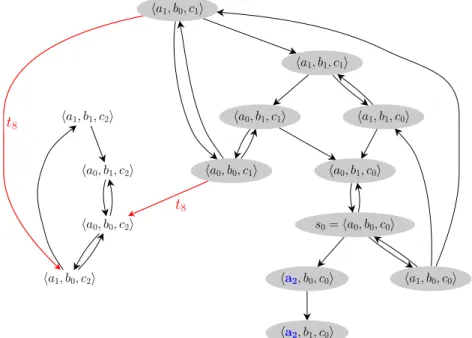
Let us consider the AN of figure 1, with s0 = ha0, b0, c0i and the goal a2.
Figure 2 shows all the possible transitions from s0. The states with a gray
back-ground are connected to a state containing a2 (in thick/blue). The transitions
in thick/red are bifurcations: once in a white state, there exist no sequence of transitions leading to a2. In other words, bifurcations are the transitions from a
gray state to a white state. In this example, t8is the (unique) local transitions
responsible for bifurcations from s0 to a2.
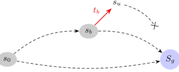
In this paper, given an AN (Σ, S, T ), we are interested in identifying the local transitions tb∈ T that trigger a bifurcation from a state reached from s0∈ S for
a given goal, describing a set of states Sg ⊆ S. We call sb a global state where
a bifurcation occurs, and su the global state after the bifurcation: su = sb· tb.
The goal is reachable from sb but not from su. This is illustrated by figure 3.
Note that, as illustrated, sb is not inevitably reached: we allow the existence of
a
0
1
2
b
0
1
c
0
1
2
b
0b
0, c
0a
1b
0b
1a
0Figure 1. An example of Automata Network (AN).‘ Automata are represented by labelled boxes, and local states by circles where ticks are their identifier within the automaton – for instance, the local state a0 is the circle ticked 0 in the box a. A
transition is a directed edge between two local states within the same automaton. It can be labelled with a set of local states of other automata. Grayed local states stand for the global state ha0, b0, c0i.
ha2, b1, c0i ha2, b0, c0i ha1, b0, c0i ha0, b0, c1i s0= ha0, b0, c0i ha1, b1, c0i ha0, b1, c0i ha1, b1, c1i ha0, b1, c1i ha1, b0, c1i ha1, b0, c2i ha0, b0, c2i ha1, b1, c2i ha0, b1, c2i t8 t8
Figure 2. Transition graph of the AN in figure 1 from the initial state s0 = ha0, b0, c0i.
The goal a2is in thick/blue; the states connected to the goal are in gray; the bifurcations
s0
sb
Sg
su tb
Figure 3. General illustration of a bifurcation. s0 is the initial state, Sg is a set of
states in which the goal local state is present. The dashed arrows represent a sequence (possibly empty) of transitions. The plain red arrow is a bifurcation from a global state sbto su, and tbis the associated local transition.
Definition 3 formalizes the notion of bifurcation, where the goal is specified by a local state g1(hence Sg= {s ∈ S | s(g) = 1}). Note that this goal specification
does not loose generality, as one can build an automaton g with local states g0
and g1, and with a local transitions from g0 to g1 conditioned by each desired
goal state.
Definition 3 (Bifurcation). Given an AN (Σ, S, T ), a global state s0∈ S and
a goal local state g1 with g ∈ Σ and g1 ∈ S(g), a bifurcation is a transition
sb tb
−→ su of the AN with sb, su ∈ S and tb ∈ T , such that s0→∗sb and ∀s0∈ S
where su→∗s0, s0(g) 6= g1.
4
Reachability and formal approximations
The identification of a bifurcation as presented in the previous section can be decomposed in three steps: we want to find sb∈ S and tb∈ T such that (1) sb is
reachable from s0(s0→∗ sb); (2) g1is reachable from sb (∃sg∈ S : sg(g) = g1∧
sb→∗sg); (2) g1is not reachable from su= sb·tb(∀s ∈ S, su→∗s ⇒ s(g) 6= g1).
Therefore, alongside the enumeration of candidate sb and tb, reachability is at
the core of our bifurcation identification.
In this section, we give a brief overview of the basics of reachability checking, stressing the methods we use in this paper.
4.1 State graph and partial order reductions
Given two states s, s0 of an AN (or an equivalent Petri net), verifying s →∗s0 is a PSPACE-complete problem [8].
The common approach for reachability checking is to build the (finite) set of all the states reachable from s until finding s0, by exploring all the possible transitions. However, such a set can be rapidly intractable with large models. Techniques relying on symbolic representations, notably using Binary Decision Diagrams (BDDs) and variants [21] can improve the scalability of this approach by several orders of magnitude [9].
In many cases, numerous transitions modelled by ANs are concurrent : their application is independent from each other. For instance, if t1and t2are
concur-rent in a state s, one can apply indiffeconcur-rently s · t1· t2 and s · t2· t1. Such features
can be exploited to provide very compact representations of the reachable states in a concurrent system, taking into account the partial order of transition applic-ations. Unfoldings, and more precisely their complete finite prefixes [13], allow to compute efficiently such compact representations.
In this paper, part of our method uses complete finite prefixes of unfoldings to compute the states that are reachable from the fixed initial state s0. Indeed,
because biological networks are typically very large, but also very sparse (each node/automaton interacts with a few others, compared to the size of the net-work), they exhibit a high degree of concurrency for their transitions, making unfolding approaches very effective.
4.2 Formal approximations
When facing a large AN, it may turn out that the reachable state space is too large for the aforementioned exact verification of reachability. Moreover, the complexity of the reachability problem can be prohibitive when numerous verifications have to be done, for instance when enumerating candidate initial states (such as sbin our case for checking goal reachability from it).
In this paper, we rely on the reachability approximations for ANs introduced in [29,15]. We will use both over-approximations (OA) and under-approximations (UA) of the reachability problem: s →∗s0is true only if OA(s →∗s0) is true and s →∗s0 is true if UA(s →∗s0) is true; but the converses do not hold in general:
UA(s →∗s0) ⇒ s →∗s0 ⇒ OA(s →∗s0)
The approximations rely on static analysis by abstract interpretation of AN dynamics. We give here the basic explanations for the over- and under-approximation. The analysis rely on the decomposition of the systems dynamics in automata, in order to derive necessary or sufficient conditions for a reachab-ility property of the form s →∗s0.
The core objects are the local paths within two local states ai, aj of a same
automaton a. We call ai aj an objective and define local-paths(ai aj) the
set of the acyclic paths of local transitions between aiand aj. Definition 4 gives
the formalization of local-paths where we use the following notations: for a local transition t = ai ` − → aj∈ T , orig(t) ∆ = ai, dest(t) ∆ = aj, enab(t) ∆ = `; ε denotes the empty sequence, and |η| is the length of sequence η.
Definition 4 (local-paths). Given an objective ai aj,
– if i = j, local-paths(ai ai) ∆
= {ε};
– if i 6= j, a sequence η of transitions in T (a) is in local-paths(ai aj) if and
only if orig(η1) = ai, dest(η|η|) = aj, ∀n, 1 ≤ n < |η|, dest(ηn) = orig(ηn+1),
We write t ∈ η⇔ ∃n, 1 ≤ n ≤ |η| : η∆ n = t. Given a local path η, eη denotes
the union of the conditions of all the local transitions composing it:
e η=∆S|η|
n=1enab(ηn)
In the AN of figure 1, local-paths(a0 a2) = {a0 b0,c0
−−−→ a2}; local-paths(c2
c1) = ∅.
Focusing on the reachability of a single local state g1 from a state s where
s(g) = 0, the analyzes essentially start with the local paths in local-paths(g0
g1): if g1 is reachable, then at least of the local path η has to be realizable,
meaning that all the local states of its conditions (eη) should be reachable. This lead to a recursive reasoning by repeating the procedure with the objectives from s to the local states inη.e
The dependence relationships between the local paths of the different auto-mata can be represented as a graph, where the nodes are all the local states, all the possible objectives, and all their local paths. Such a graph is called a Local Causality Graph (LCG), and abstracts all the executions of the AN.
From a complexity point of view, local paths are computed for each pair of local states within every automata; the length of a local path being at most the number of local states within the automaton, the number of local paths is at most polynomial in the number of local transitions and exponential in the size of the single automaton. In practice, the automata are small, typically between 2 and 4 states for biological models. Therefore, LCGs turn out to be very small compared to the reachable state space of biological networks. They have been successfully applied for analyzing dynamics of ANs with hundreds or thousands of automata, which were intractable with standard model-checking approaches [29,28].
The over-approximation and under-approximation reduce to finding sub-graphs of LCGs that satisfy some particular structural properties, which have been proven to be necessary or sufficient for the reachability property, respect-ively. Whereas the over-approximation can be verified in a time linear with the LCG [29], the under-approximation we consider in this paper requires to enu-merate over many possible sub-LCGs, but checking if a sub-LCG satisfies the sufficient condition is linear in its size.
Note that further refinements of local-paths have been considered for the mentioned approximations, but for the sake of simplicity, we stick to this coarse-grained presentation in the scope of this paper.
Appendix A gives examples of LCGs satisfying necessary or sufficient condi-tions for reachability properties in the AN of figure 1.
5
Identification of bifurcations using ASP
Among the states reachable from s0, we want to find a state sb from which (1)
the goal is reachable and (2) there exists a transition to a state from which the goal is not reachable. Putting aside the complexity of reachabilities checking, the
enumeration of candidate states sb is a clear bottleneck for the identification of
bifurcations in an AN.
Our approach combines the formal approximations and (optionally) unfold-ings introduced in the previous section with a constraint programming approach to efficiently identify bifurcations. As discussed in the previous section, checking the over-/under-approximations from candidate states and sub-LCGs is easy. For the case of unfolding, checking if a state s belongs to the state space repres-ented by a complete finite prefix is NP-complete [14]. Therefore, a declarative approach such as Answer-Set Programming (ASP) [3] is very well suited for spe-cifying admissible sb and tb, and obtaining efficient enumerations of solutions by
a solver.
We first present the general scheme of our method, and then given details on its implementation with ASP.
5.1 General scheme
A sound and complete characterization of the local transitions tb∈ T triggering a
bifurcation from state s0to the goal g1would be the following: tbis a bifurcation
transition if and only if there exists a state sb∈ S such that
(C1) su6→∗g1 (C2) sb→∗g1 (C3) s0→∗sb where su = sb· tb, s 6→∗ g1 ∆ ⇔ ∀s0 ∈ S, s →∗ s0 ⇒ s0(g) 6= g 1 and s →∗ g1 ∆ ⇔ ∃sg ∈ S : sg(g) = g1∧ s →∗sg.
However, in an enumeration scheme for sb candidates, checking reachability
and non-reachability of the goal from each sb candidate ((C1) and (C2)) is
prohibitive. Instead, we relax the above constraints as follows: (I1#) ¬OA(su→∗g1) (I2#) UA(sb→∗g1)
(I3) sb∈ unf-prefix(s0)
(I3#) UA(s0→∗sb)
where unf-prefix(s0) is the set of all reachable states from s0 represented as the
prefix of the unfolding of the AN which has to be pre-computed (section 4.1). Either (I3) or (I3#) can be used, at discretion. From OA and UA properties (section 4.2), we directly obtain:
(I1#)⇒(C1) (I2#)⇒(C2) (I3)⇔(C3)
(I3#)⇒(C3)
Therefore, our characterization is sound (no false positive) but incomplete: some tb might be missed (false negatives). Using (I3) instead of (I3#) potentially
reduces the false negatives, at the condition that the prefix of the unfolding is tractable. When facing a model too large for the unfolding approach, we should rely on(I3#)which is much more scalable but may lead to more false negatives. Relying on the unfolding from sb(unf-prefix(sb)) is not considered here, as it
would require to compute a prefix from each sb candidate, whereas unf-prefix(s0)
5.2 ASP syntax and semantics
We give a very brief overview of ASP syntax and semantics that we use in the next section. Please refer to [18,3,16] for an in-depth introduction to ASP.
An ASP program consists in a set of predicates, and logic rules of the form:
1a0 ← a1, . . ., an, not an+1, . . ., not an+k.
where ai are atoms, terms or predicates in first order logic.
Essentially, such a logical rules states that when all a1, . . . , anare true and all
an+1, . . . , an+k are false, then a0 has to be true as well. a0can be ⊥ (or simply
omitted): in such a case, the rule is satisfied only if the right hand side of the rule is false (at least one of a1, . . . , an is false or at least one of an+1, . . . , an+k
is true). A solution consists in a set of true atoms/terms/predicates with which all the logical rules are satisfied.
ASP allows to use variables (starting with an uppercase) instead of term-s/predicates: these pattern declarations will be expanded to the corresponding propositional logic rules prior to the solving. For instance, the following ASP program has as unique (minimal) solutionb(1) b(2) c(1) c(2).
2c(X) ← b(X). 3b(1).
4b(2).
In the following, we also use the notation n { a(X) : b(X) } m which is true when at least n and at most ma(X)are true whereXranges over the true b(X). 5.3 ASP implementation
We present here the main rules for implementing the identification of bifurcation transitions with ASP. A significant part of ASP declarations used by (I1#),
(I2#), (I3), and (I3#)are generated from the prior computation of local-paths
and, in the case of(I3), of the prefix of the unfolding. Applied on figure 1, our implementation correctly uncovers t8 as a bifurcation for a2.
Declaration of local states, transitions, and states Every local state ai ∈ S(a) of each automaton a ∈ Σ are declared with the predicatels(a,i).
We declare the local transitions of the AN and their associated conditions by the predicates tr(id,a,i,j) and trcond(id,b,k), which correspond to the local transition ai
{bk}∪`
−−−−→ aj ∈ T . States are declared with the predicate s(ID,A,I)
whereID is the state identifier, andA,I, the automaton and local state present
in that state. Finally, the goal g1 is declared withgoal(g,1).
For instance, the following instructions declare the automaton a of figure 1 with its local transitions, the state s0= ha0, b0, c0i, and the goal being a2:
1ls(a,0). ls(a,1). ls(a,2). 2tr(1,a,1,0).
3tr(2,a,0,1). trcond(2,b,0).
4tr(3,a,0,2). trcond(3,b,0). trcond(3,c,0).
Declaration of sb, tb, and su The bifurcation transition tb, declared asbtr(b),
is selected among the declared transitions identifiers (line 6). If ai `
−
→ aj is the
selected transition, the global state su (recall that su = sb· tb) should satisfy
su(a) = aj (line 7) and, ∀bk ∈ `, su(b) = bk (line 8). The state sb should then
match su, except for the automaton a, as sb(a) = ai (lines 9 and 10).
61 { btr(ID) : tr(ID,_,_,_) } 1. 7s(u,A,J) ← btr(ID),tr(ID,A,_,J). 8s(u,B,K) ← btr(ID),trcond(ID,B,K). 9s(b,A,I) ← btr(ID),tr(ID,A,I,_).
10s(b,B,K) ← s(u,B,K),btr(ID),tr(ID,A,_,_),B!=A.
(I1#) declaration of ¬OA(s
u →∗ g1) This part aims at finding the state
su from which g1 is not reachable. For that, we designed an ASP
implementa-tion of the reachability over-approximaimplementa-tion presented in secimplementa-tion 4.2. It consists in building a Local Causality Graph (LCG) from pre-computed local-paths. A predicateoa_valid(G,ls(A,I))is then defined upon G to be true when the local state ai is reachable from the initial state sG. The full implementation is given
in appendix B.1.
We instantiate a LCG u with the initial state su by declaring that the goal
is not reachable (oa_valid) (line 11).
11← oa_valid(u,ls(G,I)),goal(G,I).
(I2#) declaration of UA(s
b →∗ g1) This part aims at finding the state sb
from which g1 is reachable. Our designed ASP implementation of the
reachab-ility under-approximation (section 4.2) consists in finding a sub-LCG G with the satisfying properties for proving the sufficient condition. The edges of this sub-LCG are declared with the predicateua_lcg(G,Parent,Child). The graph is parameterized by (1) a context which specifies a set of possible initial states and (2) an edge from the noderoot to the local state(s) for which the simultaneous reachability has to be decided from the supplied context. The full implementa-tion is given in appendix B.2.
We instantiate the under-approximation for building a state sb from which
the goal g1 is reachable: g1 is a child of the root node of graph b (line 12).
The context is subject to the same constraints as sb from su (lines 13 and 14
reflect lines 9 and 10). Then, sb defines one local state per automaton among
the context from which the reachability of g1is ensured (line 15), and according
to lines 9 and 10.
12ua_lcg(b,root,ls(G,I)) ← goal(G,I). 13ctx(b,A,I) ← btr(ID),tr(ID,A,I,_).
14ctx(b,B,K) ← s(u,B,K),btr(ID),tr(ID,A,_,_),B!=A. 151 { s(b,A,I) : ctx(b,A,I) } 1 ← ctx(b,A,_).
(I3)declaration of sb ∈ unf-prefix(s0) Given a prefix of an unfolding from s0
(section 4.1), checking if sb is reachable from s0 is an NP-complete problem [14]
which can be efficiently encoded in SAT [22] (and hence in ASP). A synthetic description of the ASP implementation of reachability in unfoldings is given in appendix C. The interested reader should refer to [13]. Our encoding provides a predicatereach(a,i)which is true if a reachable state contains ai. Declaring sb
reachable from s0 is done simply as follows:
16reach(A,I) ← s(b,A,I).
(I3#) declaration of UA(s0 →∗ sb) An alternative to (I3) which does not
require to compute a complete prefix of the unfolding is to rely on the under-approximation of reachability similarly to (I2#). The under-approximation is instantiated for the reachability of sb from s0with the following statements:
17ua_lcg(0,root,ls(A,I)) ← s(b,A,I). 18ctx(0,A,I) ← s(0,A,I).
6
Experiments
We evaluate our method for the computation of bifurcation transitions in models of actual biological networks showing differentiation capabilities. We have selec-ted three networks showing at least two attractors reachable from a same initial state. In these cases, by supplying an adequate goal state representing one of the attractor, we expect to identify transitions causing a bifurcation from this attractor. We start by introducing our three case studies.
Immunity control in bacteriophage lambda (Lambda phage) . A number of bacterial and viral genes take part in the decision between lysis and lysogeniz-ation in temperate bacteriophages. In the lambda case, at least five viral genes (refered to as cI, cro, cII, N and cIII) and several bacterial genes are involved. We apply our method on an automata network equivalent to the model introduced in [41] and with two different goals, corresponding to lysis or lysogenization.
Epidermal Growth Factor & Tumor Necrosis Factorα(EGF/TNF) is a model
that combines two important mammalian signaling pathways induced by the Epidermal Growth Factor (EGF) and Tumor Necrosis Factor alpha (TNFα)
[24,7]. EGF and TNFα ligands stimulate ERK, JNK and p38 MAPK cascades,
the PI3K/AKT pathways, and the NFkB cascade. This network encompasses cross-talks between these pathways, as well as two negative feedback loops.
T-helper cell plasticity (Th) has been studied in [1] in order to investigate switches between attractors subsequent to changes of input conditions. It is a cel-lular network regulating the differentiation of T-helper (Th) cells, which orches-trate many physiological and pathological immune responses. T-helper (CD4+) lymphocytes play a key role in the regulation of the immune response. By APC activation, native CD4 T cells (Th0) differentiate into specific Th subtypes pro-ducing different cytokines which influence the activity of immune effector cell
Automata Network Goal (I3) (I3 #
) M-C
|pfx| |tb| Time |tb| Time |tb| Time
Lambda phage CI2 45 6 0.1s 0 0.2s 10 0.1s |Σ| = 4 |T | = 11 Cro2 3 0.1s 2 0.3s 3 0.1s EGF/TNF NFkB0 52 4 0.1s 2 0.1s 5 0.2s |Σ| = 28 |T | = 55 IKB1 3 0.1s 2 0.1s 5 0.2s Th_th1 BCL61 444 6 16s 5 23s 8 13s |Σ| = 101 |T | = 381 TBET1 5 10s 4 24s 11 14s Th_th2 GATA30 3264 7 24s 4 24s 8 60s |Σ| = 101 |T | = 381 BCL61 5 25s 4 25s 7 600s Th_th17 RORGT1 2860 9 23s 8 26s 18 48s |Σ| = 101 |T | = 381 BCL61 5 23s 4 24s 7 26s Th_HTG BCL61 OT 6 61s OT |Σ| = 101 |T | = 381 GATA31 7 34s
Table 1. Experimental results for the identification of bifurcations depending if(I3)
or (I3#)is used, compared to a exact model-checking (M-C) using NuSMV[9]. Mod-els Th_th1, Th_th2, Th_th17, Th_HTG are the same automata network but have different initial state. For each model, two different goals have been tested. |Σ| is the number of automata, and |T | the number of transitions; |pfx| is the size (number of events in the partial order structure) of the prefix of the unfolding from the initial state of the model; |tb| is the number of identified bifurcation transitions. Computation
times have been obtained on an Intel CoreR TMi7-4770 3.40GHz CPU with 16GiB of
RAM. OT indicates an out-of-time execution (more than one hour).
types. Several subtypes (Th1, Th2, Th17, Treg, Tfh, Th9, and Th22) have been well established. We report in this paper four (Pro Th1, Pro Th2, Pro Th17, Pro HTG(Th1 + Th17)) different initial state from which different attractors are reachable. The network is composed of 101 nodes and 221 interactions.
Method. For each selected model with initial state and goal, we performed the bifurcation identification following either(I1#),(I2#),(I3)(unfolding from s
0);
or (I1#), (I2#), (I3#)(reachability under-approximation). We use clingo 4.5.3 [17] as ASP solver, and Mole [38] for the computation of the unfolding ((I3)). The computation times correspond to the total toolchain duration, and includes the local-paths computation, unfolding, ASP program generation, ASP program loading and grounding, and solving. Note that the local-paths computation (and ASP program generation) is almost instantaneous for each case. Source code and models are provided in the supplementary material file.
Results. Table 1 summarizes the results of the experiments. The last exper-iment shows the limit of the exact analysis of the reachable state space: the
computation of the prefix is not tractable on this model. However, the alternat-ive approach(I3#)allows to identify bifurcation transitions in this large model. Following section 5.1, (I3#)always results in less bifurcations transitions than (I3)with our models. It can be explained with the additional approximation for the reachability of sb from s0, using the notations of section 3. One can finally
remark that when(I3)is tractable,(I3#)shows a slightly slower solving time, al-beit of the same order of magnitude. This suggest that checking if a state belongs to an unfolding is more efficient than checking its under-approximation. Finally, because there exists to our knowledge no other method for identifying bifurca-tions, we cannot compare our results with different methods, and in particular with an exact method in order to appreciate the false negative rate obtained by the(I1#)-(I2#)-(I3)scheme.
7
Conclusion
This paper presents an original combination of computational techniques to identify transitions of a dynamical system that can remove its capability to reach a (set of) states of interest. Our methodology combines static analysis of Automata Networks (ANs) dynamics, partial order representations of the state space, and constraint programming to efficiently enumerate those bifurcations. To our knowledge, this is the first intregated approach for deriving bifurcation transitions from concurrent models, and ANs in particular.
Bifurcations are key features of biological networks, as they model decisive transitions which control the differentiation of the cell: the bifurcations decide the portions of the state space (no longer) reachable in the long-run dynam-ics. Providing automatic methods for capturing those differentiations steps is of great interest for biological challenges such as cell reprogramming [12,1], as they suggest targets for modulating undergoing cellular processes.
Given an initial state of the AN and a goal state, our method first computes static abstractions of the AN dynamics and (optionnaly) a symbolic represent-ation of the reachable state space with so-called unfoldings. From those prior computations, a set of constraints are issued to identify bifurcation transitions. We used Answer-Set Programming to declare the admissible solutions and the solver clingo to obtain their efficient enumerations. For large models, the unfold-ing may be intractable: in such a case, the methods relies only on reachability over- and under-approximations. By relying on those relaxations which can be efficiently encoded in ASP, our approach avoids costly exact checking, and is tractable on large models, as supported by the experiments.
Further work will consider the complete identification of bifurcation trans-itions, by allowing false positives (but no false negatives). In combination with the under-approximation of the bifurcations presented in this paper, it will provide an efficient way to delineate all the transitions that control the reachabil-ity of the goal attractor. Future work will also focus on exploiting the identified bifurcations for driving estimations of the probability of reaching the goal at steady state, in the scope of hybrid models of biological networks [39,40].
References
1. W. Abou-Jaoudé, P. T. Monteiro, A. Naldi, M. Grandclaudon, V. Soumelis, C. Chaouiya, and D. Thieffry. Model checking to assess t-helper cell plasticity. Frontiers in Bioengineering and Biotechnology, 2(86), 2015.
2. V. Acuna, F. Chierichetti, V. Lacroix, A. Marchetti-Spaccamela, M.-F. Sagot, and L. Stougie. Modes and cuts in metabolic networks: Complexity and algorithms. Biosystems, 95(1):51–60, 2009.
3. C. Baral. Knowledge Representation, Reasoning and Declarative Problem Solving. Cambridge University Press, 2003.
4. G. Bernot, F. Cassez, J.-P. Comet, F. Delaplace, C. Müller, and O. Roux. Se-mantics of biological regulatory networks. Electronic Notes in Theoretical Com-puter Science, 180(3):3 – 14, 2007.
5. L. Calzone, E. Barillot, and A. Zinovyev. Predicting genetic interactions from boolean models of biological networks. Integr. Biol., 7(8):921–929, 2015.
6. C. G. Cassandras. Discrete event systems: modeling and performance analysis. CRC, 1993.
7. C. Chaouiya, D. Bérenguier, S. M. Keating, A. Naldi, M. P. van Iersel, N. Rodrig-uez, A. Dräger, F. Büchel, T. Cokelaer, B. Kowal, B. Wicks, E. Gonçalves, J. Dor-ier, M. Page, P. T. Monteiro, A. von Kamp, I. Xenarios, H. de Jong, M. Hucka, S. Klamt, D. Thieffry, N. Le Novère, J. Saez-Rodriguez, and T. Helikar. SBML qualitative models: a model representation format and infrastructure to foster inter-actions between qualitative modelling formalisms and tools. BMC Systems Biology, 7(1):1–15, 2013.
8. A. Cheng, J. Esparza, and J. Palsberg. Complexity results for 1-safe nets. Theor. Comput. Sci., 147(1&2):117–136, 1995.
9. A. Cimatti, E. Clarke, E. Giunchiglia, F. Giunchiglia, M. Pistore, M. Roveri, R. Se-bastiani, and A. Tacchella. NuSMV 2: An opensource tool for symbolic model checking. In Computer Aided Verification, volume 2404 of Lecture Notes in Com-puter Science, pages 241–268. Springer Berlin / Heidelberg, 2002.
10. E. M. Clarke, E. A. Emerson, and A. P. Sistla. Automatic verification of finite-state concurrent systems using temporal logic specifications. ACM Transactions on Programming Languages and Systems (TOPLAS), 8(2):244–263, 1986. 11. P. Cousot and R. Cousot. Abstract interpretation: A unified lattice model for static
analysis of programs by construction or approximation of fixpoints. In Proceedings of the 4th ACM SIGACT-SIGPLAN Symposium on Principles of Programming Languages (POPL’77), pages 238–252, New York, NY, USA, 1977. ACM. 12. I. Crespo and A. del Sol. A general strategy for cellular reprogramming: The
im-portance of transcription factor cross-repression. STEM CELLS, 31(10):2127–2135, Oct 2013.
13. J. Esparza and K. Heljanko. Unfoldings – A Partial-Order Approach to Model Checking. Springer, 2008.
14. J. Esparza and C. Schröter. Unfolding based algorithms for the reachability prob-lem. Fund. Inf., 47(3-4):231–245, 2001.
15. M. Folschette, L. Paulevé, M. Magnin, and O. Roux. Sufficient conditions for reachability in automata networks with priorities. Theoretical Computer Science, 608, Part 1:66 – 83, 2015. From Computer Science to Biology and Back.
16. M. Gebser, R. Kaminski, B. Kaufmann, and T. Schaub. Answer Set Solving in Practice. Synthesis Lectures on Artificial Intelligence and Machine Learning. Mor-gan and Claypool Publishers, 2012.
17. M. Gebser, R. Kaminski, B. Kaufmann, and T. Schaub. Clingo = ASP + con-trol: Preliminary report. In M. Leuschel and T. Schrijvers, editors, Technical Communications of the Thirtieth International Conference on Logic Programming (ICLP’14), volume arXiv:1405.3694v1, 2014. Theory and Practice of Logic Pro-gramming, Online Supplement.
18. M. Gelfond and V. Lifschitz. The stable model semantics for logic programming. In ICLP/SLP, volume 88, pages 1070–1080, 1988.
19. A. Girard, A. A. Julius, and G. J. Pappas. Approximate simulation relations for hybrid systems. IFAC Analysis and Design of Hybrid Systems, Alghero, Italy, 2006. 20. R. L. Grossman, A. Nerode, A. P. Ravn, and H. Rischel. Hybrid systems.
Springer-Verlag, 1993.
21. A. Hamez, Y. Thierry-Mieg, and F. Kordon. Building efficient model checkers using hierarchical set decision diagrams and automatic saturation. Fundam. Inf., 94(3-4):413–437, 2009.
22. K. Heljanko. Using logic programs with stable model semantics to solve dead-lock and reachability problems for 1-Safe petri nets. Fundamenta Informaticae, 37(3):247–268, 1999.
23. S. Klamt and E. D. Gilles. Minimal cut sets in biochemical reaction networks. Bioinformatics, 20(2):226–234, 2004.
24. A. MacNamara, C. Terfve, D. Henriques, B. P. Bernabé, and J. Saez-Rodriguez. State–time spectrum of signal transduction logic models. Physical Biology, 9(4):045003, 2012.
25. I. Moon. Automatic verification of discrete chemical process control systems. 1992. 26. I. Moon and S. Macchietto. Formal verification of batch processing control
pro-cedures. In Proc. PSE’94, page 469. 1994.
27. I. Moon, G. J. Powers, J. R. Burch, and E. M. Clarke. Automatic verification of sequential control systems using temporal logic. AIChE Journal, 38(1):67–75, 1992.
28. L. Paulevé, G. Andrieux, and H. Koeppl. Under-approximating cut sets for reach-ability in large scale automata networks. In N. Sharygina and H. Veith, editors, Computer Aided Verification, volume 8044 of Lecture Notes in Computer Science, pages 69–84. Springer Berlin Heidelberg, 2013.
29. L. Paulevé, M. Magnin, and O. Roux. Static analysis of biological regulatory net-works dynamics using abstract interpretation. Mathematical Structures in Com-puter Science, 22(04):651–685, 2012.
30. L. Paulevé and A. Richard. Static analysis of boolean networks based on interaction graphs: a survey. Electronic Notes in Theoretical Computer Science, 284:93 – 104, 2011. Proceedings of The Second International Workshop on Static Analysis and Systems Biology (SASB 2011).
31. E. Plathe, T. Mestl, and S. Omholt. Feedback loops, stability and multistationarity in dynamical systems. Journal of Biological Systems, 3:569–577, 1995.
32. S. Prajna. Barrier certificates for nonlinear model validation. Automatica, 42(1):117–126, 2006.
33. S. Prajna and A. Jadbabaie. Safety verification of hybrid systems using barrier certificates. In Hybrid Systems: Computation and Control, pages 477–492. Springer, 2004.
34. S. Prajna, A. Jadbabaie, and G. J. Pappas. A framework for worst-case and stochastic safety verification using barrier certificates. Automatic Control, IEEE Transactions on, 52(8):1415–1428, 2007.
35. A. Richard. Negative circuits and sustained oscillations in asynchronous automata networks. Advances in Applied Mathematics, 44(4):378–392, 2010.
36. O. Sahin, H. Frohlich, C. Lobke, U. Korf, S. Burmester, M. Majety, J. Mattern, I. Schupp, C. Chaouiya, D. Thieffry, A. Poustka, S. Wiemann, T. Beissbarth, and D. Arlt. Modeling ERBB receptor-regulated G1/S transition to find novel targets for de novo trastuzumab resistance. BMC Systems Biology, 3(1), 2009.
37. R. Samaga, A. V. Kamp, and S. Klamt. Computing combinatorial intervention strategies and failure modes in signaling networks. Journal of Computational Bio-logy, 17(1):39–53, 2010.
38. S. Schwoon. Mole. http://www.lsv.ens-cachan.fr/~schwoon/tools/mole/. 39. I. Shmulevich, E. R. Dougherty, S. Kim, and W. Zhang. Probabilistic boolean
networks: a rule-based uncertainty model for gene regulatory networks. Bioin-formatics, 18(2):261–274, feb 2002.
40. G. Stoll, E. Viara, E. Barillot, and L. Calzone. Continuous time boolean modeling for biological signaling: application of gillespie algorithm. BMC Syst Biol, 6(1):116, 2012.
41. D. Thieffry and R. Thomas. Dynamical behaviour of biological regulatory networks–ii. immunity control in bacteriophage lambda. Bulletin of mathemat-ical biology, 57:277–97, 1995 Mar 1995.
42. R. Thomas. Boolean formalization of genetic control circuits. Journal of Theoretical Biology, 42(3):563 – 585, 1973.
A
Examples of Local Causality Graphs
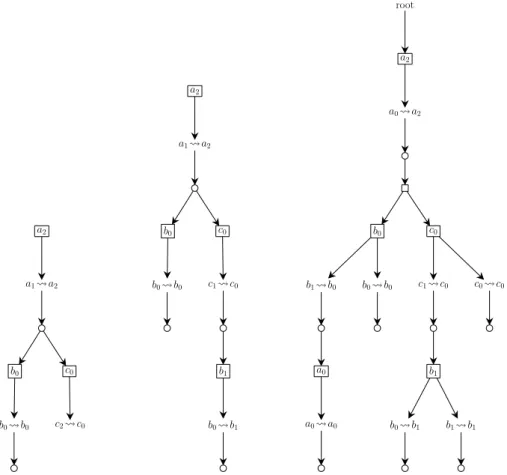
Figure 4 gives examples of Local Causality Graphs (section 4.2) for approxim-ation reachability of a2 in the AN of figure 1. The left LCG does not satisfy
the necessary condition (no local paths from c2to c0), hence a2is not reachable
from the given initial stateha1, b0, c2i. The middle LCG does satisfy the necessary
condition. And the right LCG is a valid sub-LCG for the sufficient condition for a2 reachability. a2 b0 b0 c2 c0 c0 a1 a2 b0 c1 c0 a2 b0 b1 b0 b0 c0 a1 a2 b0 b1 a2 a0 c0 b1 b0 c1 c0 b0 b1 b0 b1 b0 b0 a0 a0 b1 b1 c0 c0 a0 a2 root
Figure 4. Exemples of Local Causality Graphs for (left) over-approximation of a2
reachability from ha1, b0, c2i (middle) over-approximation of a2 reachability from
ha1, b0, c1i (right) under-approximation of a2 reachability from ha0, b1, c1i. The small
B
ASP implementation of Over- and
Under-approximation of Reachability
B.1 OA(s →∗s0): necessary condition for reachability
We propose here a possible encoding of the necessary condition for reachability in ANs outlined in section 4.2 and introduced in [29]. Starting from su(g) = g0, the
analysis starts with the local paths of the objective g0 g1: g1is reachable only if
all the conditions of the transitions of at least one local path η ∈ local-paths(g0
g1) are reachable. This recursive reasoning can be modelled with a graph relating
dependencies between objectives, local paths, and local states.
The local paths computed a priori are used to generate the template de-claration of the directed edges of the LCG oa_lcg(G,Parent,Child) from each possible objective ai aj. If local-paths(ai aj) = ∅, the objective ai aj is
linked to a nodebottom:
1oa_lcg(G,obj(a,i,j),bottom) ← oa_lcg(G,_,obj(a,i,j)).
otherwise, for local-paths(ai aj) = {η1, . . . , ηn}, we declare a node lpath for
each different local path m ∈ {1, . . . , n} as a child of ai aj:
2oa_lcg(G,obj(a,i,j),lpath(obj(a,i,j),m)) ← oa_lcg(G,_,obj(a,i,j)).
then, for each different local state bk ∈ηfm in the conditions of the local trans-itions of ηm, we add an edge from thelpath node tols(b,k):
3oa_lcg(G,lpath(obj(a,i,j),m),ls(b,k)) ← oa_lcg(G,_,obj(a,i,j)).
In the case when the local path requires no condition (ηfm= ∅, this can happen when the objective is trivial, i.e., ai ai, or when the local transitions do not
dependent on the other automata), we link thelpath to a nodetop:
4oa_lcg(G,lpath(obj(a,i,j),m),top) ← oa_lcg(G,_,obj(a,i,j)).
A LCG G for over-approximation is parameterized with a state sG: if a local
path has a local state aj in its transition conditions, the nodels(a,j)is linked,
in G, to the node for the objective ai aj (line 5), with ai = sG(a). It is
therefore required that state sGdefines a (single) local state for each automaton
referenced in G (line 6).
5oa_lcg(G,ls(A,I),obj(A,J,I)) ← oa_lcg(G,_,ls(A,I)), s(G,A,J). 61 { s(G,A,J) : ls(A,J) } 1 ← oa_lcg(G, _, ls(A, _)).
The necessary condition for reachability is then declared using the predicate
oa_valid(G,N)which is true if the node N satisfies the following condition: it is notbottom(line 7); and, in the case of a local state or objective node, one of its children isoa_valid (lines 8 and 9; or in the case of a local path, eithertop is its child, or all its children (local states) areoa_valid (lines 10 and 11).
7← oa_valid(G,bottom). 8oa_valid(G,ls(A,I)) ← oa_lcg(G,ls(A,I),X),oa_valid(G,X). 9oa_valid(G,obj(A,I,J)) ← oa_lcg(G,obj(A,I,J),X),oa_valid(G,X). 10oa_valid(G,N) ← oa_lcg(G,N,top). 11oa_valid(G,lpath(obj(a,i,j),m)) ← Vb k∈gηm oa_valid(G,ls(b,k)).
B.2 UA(s →∗s0): sufficient condition for reachability
We give here a declarative implementation of the sufficient condition for reachab-ility in ANs outlined in section 4.2 and introduced in [15]. The under-approximation consists in building a graph relating objectives, local paths, and local states which satisfies several constraints. If such a graph exists, then the related reachabil-ity property is true. Similarly to (I1#), we give template declarations for the
edges with the predicateua_lcg(G,Parent,Child). We assume that the reachab-ility property is specified by adding an edge fromrootto ls(a,i)for each local state to reach.
The graph ua_lcg is parameterized with a context which is a set of local states, declared with the predicatectx(G,A,J). Every local states aiof the graph
that are not part of the reachability specification belong to that context (line 12); and are linked to the objective aj ai for each aj in the context (line 13).
12ctx(G,A,I) ← ua_lcg(G,N,ls(A,I)), N != root.
13ua_lcg(G,ls(A,I),obj(A,J,I)) ← ua_lcg(G,_,ls(A,I)), ctx(G,A,J).
A first constraint is that each objective in the graph is linked to one and only one of its local path. Therefore, objectives without local paths (local-paths(ai
aj) = ∅) cannot be included (line 14), for the others, a choice has to be made
among local-paths(ai aj) = {η1, . . . , ηn} (line 15).
14← ua_lcg(G,_,obj(a,i,j)).
151 { ua_lcg(G,obj(a,i,j),lpath(obj(a,i,j),1..n)) } 1 ← ua_lcg(G,_,obj(a,i,j)).
As for oa_lcg, each local path is linked to all the local states composing its transition conditions: for each m ∈ {1, . . . , n}, for each bk ∈ηfm,
16ua_lcg(G,lpath(obj(a,i,j),m),ls(b,k)) ← ua_lcg(G,_,obj(a,i,j)).
The graph has to be acyclic. This is declared using a predicateconn(G,X,Y)which is true if the nodeXis connected (there is a directed path) toY(line 17). A graph is cyclic whenconn(G,X,X)(line 18).
17conn(G,X,Y) ← ua_lcg(G,X,Y). conn(G,X,Y) ← ua_lcg(G,X,Z), conn(G,Z,Y). 18← conn(G,X,X).
Then, if the node for an objective ai aj is connected to a local state ak, the
under-approximation requires ai aj to be connected with ak aj (assuming
that a has at least 3 local states, definition not shown):
19ua_lcg(G,obj(A,I,J),obj(A,K,J)) ← not boolean(A), conn(G,obj(A,I,J),ls(A,K)).
When a local transition is conditioned by at least two other automata (for in-stance c◦
ai,bj
−−−→ c•), the under-approximation requests that reaching bj does
not involve other local states from a others that ai. This is stated by the
indep(G,Y,a,i,ls(b,j)) which cannot be true if bj is connected to a local state
ak with k 6= i line 20. Then, the under-approximation requires that at most one
indep predicate is false, for a given LCG G and a given local path Y (line 21). Such an independence should also hold between the local states of the reachab-ility specification (line 22).
20indepfailure(Y,ls(A,I)) ← indep(G,Y,A,I,N), conn(G,N,ls(A,K)), K!=I. 21← indepfailure(Y,N),indepfailure(Y,M),M!=N.
22indep(G,root,A,I,ls(B,J)) ← ua_lcg(G,root,ls(A,I)),ua_lcg(G,root,ls(B,J)),B != A.
For ηm ∈ local-paths(a
i aj), for each local transition a◦ `
−
→ a• ∈ ηm, for each
couple of different local states in its condition bk, cl∈ `, bk 6= cl:
23indep(G,lpath(obj(a,i,j),m),b,k,ls(c,l)) ← ua_lcg(G,_,lpath(obj(a,i,j),m)).
C
ASP implementation of reachability in unfoldings
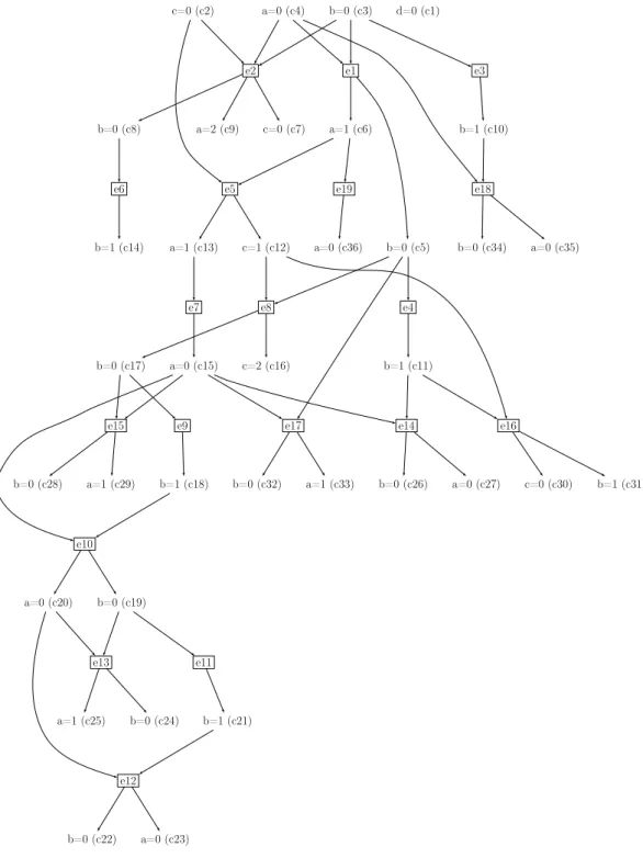
A (prefix of an) unfolding is an acyclic bipartite digraph where nodes are either events (application of a transition) or conditions (change of local state) [13]. We use the predicate post(X,Y)to denote an edge from X to Y ; andh(C,ls(A,I))
to denote that the condition C corresponds to the local state ai. Figure 5 shows
an example of unfolding.
A state s belongs to the prefix if it is possible to build a configuration such that all the local states in s have a unique corresponding condition on the cut of the configuration (line 1).
A configuration is a set of events, and we usee(E)to denote that the event E belongs to the configuration. By definition, if E is in a configuration, all its parent events are in the configuration (line 2). There should be no conflicts between two events of a configuration: two events are in conflict if they share a common parent condition (line 3).
A condition is on the cut if its parent event is in the configuration (line 4), and none of its children event is in the configuration (line 5).
11 { cut(C) : h(C,ls(A,I)) } 1 ← reach(A,I). 2e(F) ← post(F,C),post(C,E),e(E).
3← post(C,E),post(C,F),e(E),e(F),E != F. 4e(E) ← cut(C),post(E,C).
e5 c=0 (c2) d=0 (c1) e19 e18 e11 c=0 (c7) e13 e12
e15 e17 e14 e16
b=0 (c19) b=1 (c18) e3 a=0 (c35) b=0 (c34) b=1 (c11) b=1 (c10) b=0 (c17) c=2 (c16) a=1 (c33) b=0 (c32) b=1 (c21) a=1 (c13) a=2 (c9) b=0 (c8) e9 e8 c=1 (c12) b=0 (c3) e4 e7 e6 e1 a=1 (c6) b=0 (c5) a=0 (c4) b=0 (c22) a=0 (c23) a=0 (c20) a=0 (c36) b=0 (c26) a=0 (c27) b=0 (c24) a=1 (c25) b=1 (c31) b=0 (c28) a=1 (c29) c=0 (c30) a=0 (c15) e10 b=1 (c14) e2
Figure 5. Unfolding of the AN of figure 1. Events are boxed nodes, conditions have no borders and indicate both the automata local state and the condition identifier.
![Table 1. Experimental results for the identification of bifurcations depending if (I3) or (I3 # ) is used, compared to a exact model-checking (M-C) using NuSMV[9]](https://thumb-eu.123doks.com/thumbv2/123doknet/8236633.277041/15.892.202.735.173.481/table-experimental-results-identification-bifurcations-depending-compared-checking.webp)