• Aucun résultat trouvé

Synchronization on the circle

N/A
N/A
Protected

Academic year: 2021

Partager "Synchronization on the circle"

Copied!
21
0
0

Texte intégral

(1)

Synchronization on the circle

Alain Sarlette, Rodolphe Sepulchre

January 16, 2009

Abstract

The goal of the present paper is to highlight the fundamental differences of so-called

synchronization or consensus algorithms when the agents to synchronize evolve on a compact homogeneous manifold (like the circle, sphere or the group of rotation matrices), instead of a

vector space. For the benefit of understanding, the discussion is restricted to the circle. First, a fundamental consensus algorithm on Rnis reviewed, from which continuous- and discrete-time synchronization algorithms on the circle are deduced by analogy. It is shown how they are connected to Kuramoto and Vicsek models from the literature. Their convergence properties are similar to vector spaces only for specific graphs or if the agents are all located within a semicircle. Examples are proposed to illustrate several other possible behaviors. Finally, new algorithms are proposed to recover (almost-)global synchronization properties.

1

Introduction

During the last decades, synchronization phenomena have attracted the attention of numerous researchers from various fields. Many recent engineering applications consider swarms of agents that combine their efforts in a coordinated (“synchronized”) way to achieve a common task, e.g. distributed exploration [6, 15] or interferometry [1, 16]. From a modeling and analysis viewpoint, collective phenomena are studied by both the theoretically oriented communities of dynamical systems and statistical physics, as well as more practically oriented experimental physics and biology communities (see e.g. [7, 14, 30, 32]). Celebrated examples of simplified models for the study of coordination phenomena include Kuramoto and Vicsek models.

Kuramoto model is proposed in [14] to describe the continuous-time evolution of phase variables in a population of weakly coupked oscillators. Each agent k is considered as a periodic oscillator of natural frequency ωk, whose phase — i.e. position on its cycle — at time t is θk(t) ∈ S1. In

addition to its natural evolution, each agent is coupled to all the others:

d dtθk= ωk+ N X k=1 sin(θj− θk) , k = 1, 2, ..., N . (1)

Vicsek model is proposed in [32] to describe the discrete-time evolution of interacting particles that move with unit velocity in the plane. In the absence of noise, the model writes

rk(t + 1) = rk(t) + eiθk(t) (2) θk(t + 1) = arg   X j∈nk(t) eiθj(t) + eiθk(t) , k = 1, 2, ..., N , (3)

where θk denotes the heading angle of particle k and rk its position in the (complex) plane. The

set nk(t) is defined to contain all agents j for which krk(t) − rj(t)k ≤ R for some fixed R > 0,

such that agent k is only influenced by “close enough” fellows1.

1Notation kzk denotes the complex norm of z ∈ C, such that z = kzk ei arg(z). The present paper uses the convention that arg(0) can take any value on S1. It canonically identifies C ∼= R2, yielding kzk =zTz for z ∈ R2.

(2)

In the engineering community, synchronization has focused on several basic problems. One of them is for a set of agents to reach agreement on some “quantity” — e.g. a position, velocity,. . . — while exchanging information along a limited set of communication links. This so-called consensus

problem has been extensively studied for quantities on the vector space Rn, see e.g. [2, 17, 18, 20,

21, 31] and [19] for a review; related results are briefly explained in the next section. However, it appears that many interesting engineering applications and phenomenological models, e.g. as presented above, involve nonlinear manifolds; this includes distributed exploration of a planet (sphere S2), rigid body orientations (special orthogonal groups SO(2) or SO(3)), and collective

motion on limit cycles (abstracted as a circle S1).

Vicsek and Kuramoto models illustrate two general types of problems for synchronization on manifolds. In Vicsek model, stabilizing parallel motion requires equal orientations of the agents, which comes down to reaching agreement on states θk on the circle. In Kuramoto model, moving

with fixed relative phases corresponds to reaching agreement on a motion on the circle. On multi-dimensional manifolds, coordinated motion becomes more complex than on S1 where it simply

comes down to reaching agreement on a frequency in R; this is the subject of [22]. The present paper focuses on state agreement, more commonly called synchronization.

Definition 1.1: A swarm of N agents with states xk(t) ∈ M evolving on a manifold M, k =

1, 2, ..., N , is said to asymptotically synchronize or reach synchronization if

x1= x2= ... = xN asymptotically.

The asymptotic value of the xk is called the consensus value.

The circle is probably the simplest nonlinear manifold to highlight the specifities of synchro-nization on highly symmetric compact nonlinear spaces. Therefore the present paper focuses on the circle and mentions extensions to manifolds at the end. An important aspect is to maintain the symmetry of the synchronization problem: the behavior of the swarm must be invariant with respect to a common translation of all the agents (i.e. on S1, under the transformation θ

k→ θk+a

∀k ∈ V); therefore extensions consider manifolds on which “all points are equivalent” — formally, compact homogeneous manifolds like Sn, SO(n) or the Grassmann manifolds. In order to

concen-trate on fundamental issues of synchronization and geometry, system dynamics are simplified to first-order integrators.

The paper is organized as follows. Section 2 briefly reviews a fundamental algorithm for synchronization on vector spaces, also known as a “consensus algorithm”, in continuous- and discrete-time. Section 3 extends this algorithm to the circle and highlights its link with Kuramoto [14] and Vicsek [32] models. Section 4 reviews the positive synchronization properties of these algorithms. Section 5 illustrates the fact that, in contrast to vector spaces, convergence to non synchronized behavior is possible on the circle. Section 6 presents three recently proposed algo-rithms for (almost-)global synchronization on the circle: a modified coupling function, a gossip

algorithm where agents randomly select or discard information from their neighbors, and an

al-gorithm based on auxiliary variables. Section 7 briefly mentions extensions of the framework to compact homogeneous manifolds. General notations and background information about graphs can be found in the Appendix. Proofs are summarized to their main ideas; complete versions can be found in corresponding references and in [25].

2

Consensus algorithms on vector spaces

The study of synchronization on vector spaces is a widely covered subject in the systems and control literature of the last decade. The material in the present Section is a summary of basic results developed in this framework by several authors, including [2, 17, 18, 20, 21, 31]; see [19] for a review and [18] for some examples of applications.

(3)

Consider a swarm of N agents with states xk ∈ Rn, k ∈ V = {1, 2, ..., N }, evolving under continuous-time dynamics d dtxk(t) = uk(t) , k = 1, 2..., N (4) or discrete-time dynamics xk(t + 1) = xk(t) + uk(t) , k = 1, 2..., N (5)

where uk is a coupling term. The goal is to design uk such that the agents asymptotically

syn-chronize in the sense of Definition 1.1, with the following restrictions.

1. Communication constraint: uk may only depend on information concerning agent k and the

agents j à k sending information to k according to some imposed communication graph G (see Appendix).

2. Configuration space symmetry: the behavior of the coupled swarm must be invariant with respect to uniform translation of all the agents: defining yk(0) = xk(0) + a ∀k ∈ V for any

a ∈ Rn, it must hold y

k(t) = xk(t) + a ∀k ∈ V and ∀t ≥ 0. Therefore uk may only depend

on the relative positions of the agents, i.e. on (xj− xk) for j à k.

3. Agent equivalence symmetry: all the agents in the swarm must be treated equivalently. This implies that (i) the form of uk must be the same ∀k ∈ V and (ii) all j à k must be treated

equivalently in uk.

This problem is traditionally called the consensus problem on a vector space. On manifolds, the term “synchronization problem” is preferred because the term “consensus” can be given a partic-ular meaning different from synchronization, see [23]. On vector spaces, “consensus” as defined in [23] is equivalent to synchronization, so both terms can be used interchangeably.

The consensus problem on vector spaces is solved by the linear coupling

uk(t) = α N

X

j=1

ajk(t)(xj(t) − xk(t)) , k = 1, 2..., N (6)

where ajk is the weight of link j à k and α is a positive gain. The intuition behind (6) is that

each agent moves towards its neighbors, in agreement with the traditional meaning given to a “consensus” process. In continuous-time, the closed-loop system (4),(6) implies that agent k is moving towards the position in Rn corresponding to the (positively weighted) arithmetic mean of

its neighbors, 1 d(i)k P jÃkajkxj, where in-degree d (i) k = P

jÃk ajk. In discrete-time, α must satisfy

α d(i)k (t) ≤ b for some constant b < 1, ∀k ∈ V. Then (5),(6) means that the future position of agent k is at the (positively weighted) arithmetic mean 1

βk+d(i)k

(PjÃkajkxj+βkxk) of its neighbors

j à k and itself, with non-vanishing weight βk.

Clearly, (6) satisfies the three constraints mentioned above.

The convergence properties of the linear consensus algorithm on a vector space are well char-acterized. An extension of the following basic result in the presence of time delays can be found in [20]; the present paper does not consider time delays.

Proposition 2.1: (adapted from [17, 18, 20, 31]) Consider a set of N agents evolving on Rn

according to (continuous-time) (4),(6) with α > 0 or according to (discrete-time) (5),(6) with αd(i)k (t) ∈ [0, b] ∀t ≥ 0 and ∀k ∈ V, for some constant b ∈ (0, 1). Then the agents globally and

exponentially converge to synchronization at some constant value ¯x ∈ Rnif and only if the

commu-nication among agents is characterized by a (piecewise continuous) δ-digraph which is uniformly connected.

If in addition, G is balanced for all times, then the consensus value is the arithmetic mean of the initial values: ¯x = 1

N

PN

k=1xk(0).

Proof idea: For the first part, see [17, 18], or equivalently [2] or [31]. For the second part, it is easy to see that for a balanced graph, 1

N

PN

(4)

then obtained by comparing its value for t = 0 and for t going to +∞. ¤ The proof of Proposition 2.1 essentially relies on the convexity of the update law: the position of each agent k for t > τ always lies in the convex hull of the xj(τ ), j = 1, 2, ..., N . The permanent

contraction of this convex hull, at some nonzero minimal rate because weights are non-vanishing, allows to conclude that the agents end up at a consensus value. An obvious negative consequence of Proposition 2.1 for non-varying G is that synchronization cannot be reached if G is not root-connected.

If interconnections are not only balanced, but also undirected and fixed, then the linear con-sensus algorithm is a gradient descent algorithm for the disagreement cost function

Vvect(x) = 12 N X k=1 N X j=1 ajkkxj− xkk2= k(B ⊗ In)xk2= xT(L ⊗ In)x (7)

where kzk denotes the Euclidean norm√zTz of z ∈ Rm, B and L are the incidence and Laplacian

matrices of G respectively (see Appendix), x ∈ RN ndenotes the vector whose elements (k −1)n+1

to kn contain xk, and ⊗In is the Kronecker product by the n × n identity matrix.

3

Consensus algorithms on the circle

Consider a swarm of N agents with states on the circle S1. The global topology of the circle

is fundamentally different from vector spaces, because if θk denotes an angular position on the

circle, then θk + 2π = θk, that is, translations on the circle are defined modulo 2π because they

correspond to rotations. This difference in topology, imposing a non-convex configuration space, fundamentally modifies the synchronization problem.

The synchronization problem on S1 is considered under the same agent dynamics as on Rn,

i.e. (4) or (5) with xk replaced by θk. However, for the design of uk, the different topology induces

different implications of the configuration space symmetry. The behavior of the swarm must (i) be invariant with respect to a uniform translation of all θk and (ii) be invariant with respect to the

translation of any single θk by a multiple of 2π — i.e., if φk(0) = θk(0) + 2aπ for some k ∈ V and

a ∈ Z, and φj(0) = θj(0) ∀j 6= k, then it must hold φk(t) = θk(t) + 2aπ ∀t ≥ 0 and φj(t) = θj(t)

∀j 6= k and ∀t ≥ 0. This implies that uk may only depend on 2π-periodic functions of the relative

positions (θj − θk) of the agents j à k. The simple linear algorithm (6) does not satisfy the

periodicity required for configuration space symmetry, and therefore cannot be used on the circle. It can however be used to derive algorithms for synchronization on S1that are similar to (6) when

all agents are within a small arc of the circle. The discrete-time and continuous-time cases are treated consecutively. Because of the symmetry with respect to uniform translations on S1, the

swarm’s behavior is entirely characterized by examining the evolution of relative positions. Definition 3.1: A configuration is a particular set of relative positions of the agents. Thus a

configuration is equivalent to a point (¯θ1, ¯θ2, ..., ¯θN) ∈ S1× S1× ... × S1 and all the points obtained

by its uniform rotations (¯θ1+ a, ¯θ2+ a, ..., ¯θN + a) for a ∈ S1.

3.1

Discrete-time

Synchronization of θk ∈ S1, k = 1, 2, ..., N , can be seen as synchronization of xk ∈ R2 under

the constraint kxkk = 1. If the xk were not restricted to kxkk = 1, algorithm (5),(6) would

impose xk(t + 1) =β 1

k+d(i)k

³PN

j=1ajkxj(t) + βkxk(t)

´

, k = 1, 2, ..., N , with some non-vanishing

βk(t) > 0. With this update law, xk(t + 1) does generally not satisfy kxk(t + 1)k = 1. To obtain

kxk(t + 1)k = 1, the result of algorithm (5),(6) is projected onto the unit circle. Identifying

(5)

synchronization algorithm θk(t + 1) = arg  XN j=1 ajkeiθj(t) + β eiθk(t) , k = 1, 2, ..., N , (8)

for some constant β > 0. The update of one agent according to (8) is illustrated on Figure 1. It is clear from the picture that (8) respects the geometric invariance of S1. This is confirmed by

rewriting (8) as θk(t + 1) = θk(t) + uk = θk(t) + arg   N X j=1 ajkei(θj(t)−θk(t)) + β , k = 1, 2, ..., N (9)

where ukindeed only involves 2π-periodic functions of relative positions of connected agents j à k.

-<e 6 =m u θ1Ãk(t) u θ2Ãk(t) u θk(t) ©© ©© ©© ©© ©©b ¢ ¢ ¢ ¢ ¢ ¢ b b AA AA AA pk ¶¶ ¶¶ ¶ uθk(t + 1) S S ouk(t)

pk:= 1.5eiθk+ eiθ1+ eiθ2

Figure 1: Illustration of update law (8) for one agent k with β = 1.5 and a1k= a2k = 1.

For fixed undirected G, the point θk(t + 1) obtained from (8) is the projection on the unit circle

of a point obtained by gradient descent for Vvect in the complex plane.

Vicsek model: Heading update law (3) actually corresponds to (8) with β = 1 and ajk

{0, 1}. The positions define the interconnection graph G(t) by imposing ajk = 1 if and only if

krk(t) − rj(t)k ≤ R; therefore G is called a proximity graph. The study of proximity graphs, or

other state-dependent graphs, is beyond the scope of the present work.

3.2

Continuous-time

Taking the continuous-time limit of (8) amounts to letting β grow indefinitely. In this limit case,

xk(t + 1) ∈ C is defined with an infinitesimal gradient step for Vvect, and projected onto S1 to

yield θk(t + 1). This is strictly equivalent to projecting the gradient of Vvect onto the tangent to

the circle at θk(t), and taking a corresponding infinitesimal descent step along the circle. Thus by

viewing Vvect as a function of θ, renamed for clarity

Vcirc(θ) = 12 N X k=1 N X j=1 ajkkeiθj − eiθkk2=12 N X k=1 N X j=1 ajk ³ 2 sin(θj−θk 2 ) ´2 , (10)

the corresponding gradient descent algorithm along the circle, d

dtθk = −α∂V∂θcirck ∀k ∈ V with α > 0, is the continuous-time limit of (8). Computing the gradient of (10) yields the following

continuous-time algorithm for synchronization on the circle, with constant α > 0:

d dtθk= α N X j=1 (ajk(t) + akj(t)) sin(θj(t) − θk(t)) , k = 1, 2, ..., N . (11)

(6)

This algorithm can only be implemented for undirected G. An extension to directed graphs is d dtθk = 2α N X j=1 ajk(t) sin(θj(t) − θk(t)) , k = 1, 2, ..., N . (12)

This is the actual algorithm considered in the following. It satisfies the geometric invariance of

S1, since the right-hand side is a 2π-periodic function of relative positions. With x

k = eiθk, (12) is equivalent to d dtxk = 2α Projxk   N X j=1 ajk(xj− xk)   (13) where Projxk(rk) = rk − xkx T

krk denotes the orthogonal projection of rk ∈ C ∼= R2 onto the

direction tangent to the unit circle at xk= eiθk. The geometric interpretation is that (13) defines a

consensus update similar to (4),(6) but constrained to the subset of R2where kx

kk = 1. Algorithm

(12) was proposed in [28] in a control framework, and is directly linked to Kuramoto model. Kuramoto model: Comparing with (1), algorithm (12) in fact corresponds to Kuramoto model with equal natural frequencies ω1= ω2= ... = ωN, but general interconnections. This highlights

a link between the sine-model of Kuramoto and the “averaging” update law for headings in Vicsek model. For the complete graph, Vcirc = 12

PN k=1 PN j=1keiθj − eiθkk2 = N2 ° ° °PNk=1eiθk ° ° °2 . The quantity ° ° °PNk=1eiθk ° °

°2, known as the “complex order parameter” in the context of Kuramoto model, has been used for decades as a measure of the synchrony of phase variables in the literature on coupled oscillators.

The main point in studies of Kuramoto model is the coordination of agents having different

ωk. The important issue of robustly coordinating agents despite their different natural tendencies

is not the subject of the present paper.

4

Convergence properties

Section 3 proposes algorithms (8) and (12) as natural extensions of synchronization algorithms for the circle. However, the circle is not a convex configuration space. As a consequence, the convergence properties of (8) and (12) do not match those of (4),(6) and (5),(6) on vector spaces. The present Section focuses on positive convergence results, while Section 5 focuses on situations in which asymptotic synchronization is not achieved.

4.1

Local synchronization like for vector spaces

When all agents are within a small subset of S1, (12) becomes similar to (4),(6) because sin(θ

j−

θk) ' (θj− θk) for small (θj− θk). A similar observation can be made for the discrete-time

algo-rithms. It is thus not surprising that [12, 18] are able to show that asymptotic synchronization on the circle is locally achieved under the same conditions as on vector spaces.

Proposition 4.1: (adapted from [18]) Consider a set of N agents evolving on S1 according to

(continuous-time) (12) with α > 0 or according to (discrete-time) (8) with β > 0. If the communi-cation among agents is characterized by a (piecewise continuous) δ-digraph G which is uniformly connected and all agents are initially located within an open semicircle, then they exponentially converge to synchronization at some constant value ¯θ ∈ S1.

Proof idea: Assume without loss of generality that θk∈ [−b, b] ⊂ (−π22) initially. Then sin(θk(t)−

(7)

equivalent to d dtθk= α N X j=1 ajk(t) cjk(t) (θj(t) − θk(t)) (14)

for some time-varying cjk≥ sin(2b)2b > 0. This can be viewed as a linear synchronization algorithm

for θ ∈ R with a δ2-digraph G2of weights (ajkcjk). A similar idea can be used in discrete-time. ¤

When the agents are distributed over more than a semicircle, the proof of Proposition 4.1 no longer holds, because the cjk can be negative. This is in fact the consequence of a loss of

convexity, implying that the strong vector space arguments of [17, 18] are no longer applicable2.

In algorithms (8) and (12), agents move on the shortest path towards their neighbors. Therefore, if the agents are initially located within a semicircle, then they remain within this set for all future times, while agents distributed over more than a semicircle may, a priori, leave any open arc s ∈ S1

containing them all. A more global analysis requires stronger assumptions.

4.2

Some graphs ensure (almost) global synchronization

For general graphs, synchronization is only locally asymptotically stable. For some graphs how-ever, synchronization is (almost) globally asymptotically stable.

Proposition 4.2: (adapted from [4, 29]) Consider a set of N agents evolving on S1 by applying

(12) with α > 0 or (8) with β > 0 not too small (see Propositions 5.2 and 5.3 in the following section). If communication graph G is either a fixed directed root-connected tree, or an undirected tree, or the complete graph, or any vertex-interconnection of trees and complete graphs3, then the

agents asymptotically converge to synchronization, for almost all initial conditions.

Proof idea: For the directed rooted tree, each agent is attracted towards its parent and, except for unstable situations where two connected agents are exactly at opposite positions on the circle, they synchronize at the initial position of the root. The particular undirected graphs have the property that synchronization is the only local minimum of Vcirc. This is rather obvious for the

tree, from the fact that for any pair of connected agents, variations of Vcirc can be built involving

only the distance between that particular pair of agents. The property is proved for the complete graph in [29]. Finally, [4] shows that the property holds for vertex-interconnections of graphs for which it holds individually. Then Propositions 5.1, 5.2 and 5.3 of the following section ensure that synchronization is the only stable limit set. ¤

5

Obstacles to global synchronization

Section 4 identifies situations where (8) and (12) converge to synchronization. The present section examines what can happen when this is not the case.

5.1

Convergence to local equilibria for fixed undirected G

The fact that for fixed undirected G, (12) is a gradient descent for Vcirc, has strong implications

for the convergence analysis.

Proposition 5.1: Consider a set of N agents evolving on S1 according to (12) with α > 0,

with communication graph G fixed and undirected. Then the agents always converge to a set of 2An open subset s ⊂ S1is convex if it contains all shortest paths between any two points of s.

3A vertex-interconnection of two graphs G

1(V1, E1) and G2(V2, E2) is a graph G whose vertices can be partitioned

into a singleton {k} and two sets Va, Vband whose edge set can be partitioned into two sets Ea, Eb, such that

(8)

equilibria corresponding to the critical points4 of V

circ defined in (10). The only asymptotically

stable equilibria are the local minima of Vcirc.

Proof idea: Properties of gradient algorithms. ¤ For the discrete-time algorithm, in addition to a result similar to Proposition 5.1 but with a bound on β, it can be shown that under locally asynchronous update, convergence holds for arbi-trary β, i.e. without requiring any minimal inertia. Agents are said to update synchronously if, between instants t and t+1, all agents k ∈ V apply (8). In contrast, agents are said to update locally

asynchronously if, between instants t and t + 1, only a subset of agents σ ⊂ V applies (8) and the

others remain at their position, and set σ contains no agents that are connected to each other in G. Proposition 5.2: (from [24]) Consider a set of N agents evolving on S1 by applying (8) locally

asynchronously with update subset sequence σ(t), for β > 0 and fixed undirected G. Assume that there exist a finite time span T and a partition of the discrete-time space [t0, t1) , [t1, t2),... with

(tn+1− tn) < T ∀n ∈ Z≥0, such that ∀k ∈ V and ∀n ∈ Z≥0, there exists t ∈ [tn, tn+1) such that

k ∈ σ(t). Then the agents almost always converge to a set of equilibria corresponding to the critical points of Vcirc. The only asymptotically stable equilibria are the local minima of Vcirc.

Proof idea: Under the assumptions of the Proposition, denotingPNj=1ajkei(θj−θk)+ β = ρkeiuk,

Vcirc(t + 1) − Vcirc(t) = −2 X k∈σ(t) (ρk+ β) ¡ sin(uk 2) ¢2 ≤ 0 .

Since every agent k is updated at an infinite number of time instants, uk or ρk (making uk

unde-fined) must go to 0 when t goes to +∞, ∀k ∈ V. The case ρk = 0 has zero measure and can only

appear “by chance”, because it is the global maximum of Vcirc with respect to θk. If uk goes to

0, then agent k asymptotically approaches an equilibrium set; only minima can be asymptotically

stable for a descent algorithm. ¤

For synchronous update, it is again necessary to impose a bound on the motion of the agents. However this bound is not easy to find. The following result provides a conservative bound on β. Proposition 5.3: (from [24]) Consider a set of N agents evolving on S1 by applying (8)

syn-chronously with fixed, undirected and unweighted G. Assume that β ≥ dmax(M2+ 1) where e M ∗−1 M∗ = 1 +ddmax sum with dsum= PN j=k d (i)

k and dmax= maxk∈V(d(i)k ), where d

(i)

k is the in-degree of agent k. Then the

agents almost always converge to a set of equilibria corresponding to the critical points of Vcirc.

The only asymptotically stable equilibria are the local minima of Vcirc.

Proof idea: The proof shows that Vcirc(t + 1) − Vcirc(t) ≤ 0 for synchronous operation and the

bound on β. See [24] or [25] for complete computations. ¤ A problem with the bound of Proposition 5.3 is that each agent must know dsum and dmax,

which is information about the (communication structure of the) whole swarm.

In the absence of inertia (β = 0), (8) can lead to a limit cycle in synchronous operation, at least for some G (see [25] for an example).

Hopfield network: This model proposed in [11] considers N neurons with states xk ∈ {−1, 1}.

The discrete-time update law for the states of the neurons is

xk(t + 1) = sign   N X j=1 ajkxj(t) + ξk , 1, 2, ..., N (15)

(9)

where ξk is a firing threshold. Considering VH = −12 PN k=1 PN j=1 ajkxjxk− PN k=1xkξk , [11]

shows that when (15) is applied asynchronously with a random update sequence, the property

VH(t + 1) ≤ VH(t) always holds and the network eventually reaches a local minimum of VH. In

contrast, the system can go into a limit cycle under synchronous operation (see [10]). Defining the sphere Sn of dimension n as {x

k ∈ Rn+1 : kxkk = 1}, the set {−1, 1} can be

seen as “ S0 ”, while the circle is S1. For ξ

k = 0, (15) is in fact the strict analog of (8) for “the

sphere of dimension 0” — namely moving towards the neighbors in the embedding vector space and projecting back to the state space. The absence of inertia in (15) would correspond to β = 0 in (8). Both (8) and (15) can be viewed as projections of descent algorithms for a symmetric quadratic potential, which remain descent algorithms under locally asynchronous update such that convergence is ensured. Both algorithms can fail to converge and run into a limit cycle in synchronous operation.

Propositions 5.1, 5.2 and 5.3 say that the stable equilibria are the minima of Vcirc.

Unfortu-nately, depending on G, there may be local minima different from synchronization.

Local equilibria for the undirected ring: The following example is taken from [13]. Consider

N agents interconnected according to an undirected, unweighted ring graph. Then the critical

points of Vcirc satisfy sin(θja(k)− θk) + sin(θjb(k)− θk) = 0 where ja(k) and jb(k) are the two

neighbors of k in the ring graph. This requires positions of consecutive agents in the ring graph to differ either by θ0 or by π − θ0, for some θ0 ∈ [0,π2] well chosen such that the sum of all

angle differences is a multiple of 2π. Stability of these equilibria can be assessed by examining the Hessian of Vcirc. This leads to the conclusion that each configuration with |θj− θk| = θ02

∀(j, k) ∈ E is locally asymptotically stable under (12) or (8), and all other configurations are

unstable. Thus in a stable configuration, consecutive agents in the ring graph are separated by θ0

on the circle, for some θ0∈ (−π22) satisfying N θ0= 2aπ with a ∈ Z. The case θ0= 0 corresponds

to synchronization. When N ≥ 5, stable configurations exist with θ0 6= 0, see Figure 2. For all

these configurations,PNk=1 eiθk= 0, therefore they are said to be balanced.

v v v v v v v v v v v v v v v v 1 = 6 2 = 7 3 = 8 4 = 9 5 = 10 1 2 1 3 4 5 6 7 8 9 10 5v 6 v v9 2 v v v 4 7 v v 8 3

Figure 2: Several balanced configurations that are stable for the undirected ring graph; agents are numbered in the order of the ring, e.g. agent 3 is connected to agents 2 and 4.

Stable configurations are graph dependent: It is currently an open question to character-ize, with graph-theoretic properties, which graphs admit no local minima of Vcirc different from

synchronization. The following result shows that in fact, any configuration that is sufficiently “spread” on the circle is stable under the synchronization algorithms for a well-chosen weighted digraph.

(10)

Proposition 5.4: Consider a set of N agents distributed on S1 in a configuration {θ

k} such that

for every k, there is at least one agent located in (θk, θk+ π/2) and one located in (θk− π/2, θk);

such a configuration requires N ≥ 5. Then there exists a positively weighted and strongly connected δ-digraph making this configuration locally exponentially stable under (12) with α > 0.

Proof idea: Choose nonzero weights ajk only for the θj ∈ (θk− π/2, θk+ π/2), and such that

rk:=

PN

j=1ajk(xj− xk) is aligned with xk= eiθk. ¤

For any of the weight choices that locally stabilize specific configurations, synchronization is also exponentially stable — but thus only locally. The equilibrium configurations of (8) and (12) different from synchronization are formalized in [23] as consensus configurations. The same paper also considers the related problem of “spreading” agents on the circle, which is formalized with the notions of anti-consensus and balancing configurations.

Structurally stable divergent behavior in Vicsek model: The above example of stable equilibria for the undirected ring allows to illustrate a situation where Vicsek model diverges. Consider N ≥ 5 agents initiated as in Figure 3: (i) initial positions rk(0) ∈ R2 are regularly

distributed on a circle such that each agent can sense only its immediate neighbor on the left and on the right; (ii) initial orientations θk(0) ∈ S1point radially outwards of the circle formed by the

positions. Then the update equation for agent orientations θk(t) is exactly in a stable configuration

different from synchronization under a ring interconnection graph. The agents move radially outwards; at a particular time step, all communication links drop. Stability of the equilibrium for the orientations and the fact that all communication links still disconnect at the same instant when positions are slightly shifted ensures that the divergent behavior is observed in an open neighborhood of initial conditions around this ideal situation. Examining stable equilibria of (8) and (12) for G different from an undirected ring, one sees that the stable divergent behavior remains if the sensing regions are increased such that each agent initially has several neighbors on the left and on the right.

1 v v v v v v v v v ? ­ ­ À JJ^ » » 9 XXz H H Y ©©* A AK ¢¢¸

Figure 3: Initial conditions for divergent behavior in Vicsek model. The black disks denote agent positions, arrows denote orientations; the circle represents the sensing region of agent 1.

5.2

Limit sets different from equilibrium

Section 5.1 lists cases where (12) or (8) do not converge to synchronization, but still to a set of equilibria. There are also cases where the agents do not converge to a set of equilibria.

For fixed undirected graphs, the swarm is ensured to converge to a set of equilibria, except for the discrete-time algorithm when β is too small (see Proposition 5.3). In the latter case, behavior

(11)

0 50 100 150 200 250 300 15 20 25 30 35 40 time θk (degrees)

Figure 4: Illustration of disorderly-looking quasi-periodic motion of an agent k for which d dtθk =

P3

j=1 sin(θj− θk) where θ1belongs to a regularly spaced undirected ring, dtdθ1= 0; θ2is in cyclic

pursuit with 5 other agents, d dtθ2=

3; θ3is in cyclic pursuit with 11 other agents, dt3= 1.

of (8) is not as clear and the system may run into a limit cycle; see [24] or [25] for details. Periodic and quasi-periodic behaviors can easily be constructed for (12) with fixed directed graphs.

The simplest such behavior is called cyclic pursuit: each agent k is attracted by its neighbors to move (say) clockwise, and the agents keep turning without synchronizing. A classical situation of stable cyclic pursuit is a directed ring graph with consecutive agents separated by

N.

In basic cyclic pursuit, agents keep moving on the circle but relative positions remain constant. A more meaningful periodic behavior occurs when relative positions periodically vary in time. Such situations can be built with agents partitioned into two sets such that each set is in cyclic pursuit at a different velocity. Start for instance with two unweighted directed ring graphs of N1 and N2

agents, where N1+ N2= N and N1 6= N2; consecutive agents in each ring are separated by N1

and

N2. Then the resulting behavior is satisfactory, but the overall graph is not connected. To

obtain a strongly connected graph, each agent of the first ring can be coupled to all the agents of the second ring and conversely; indeed, for a set of regularly spaced agents Pk eiθk = 0, so

coupling an agent to such a set does not change its behavior.

Likewise, a quasi-periodic variation of relative positions is obtained when several sets of agents move in cyclic pursuit with irrational velocity ratios. This can be built for instance with unitary graph weights and α = 1, if one set has x agents in a splay state for an undirected ring graph ⇔

d

dtθk = 0, a second set has 6 agents in cyclic pursuit with a directed ring graph ⇔ dtdθk=

3, and a third set has 12 agents in cyclic pursuit with a directed ring graph ⇔ d

dtθk = 1.

Finally, an example of disorderly-looking quasi-periodic motion can be built by adding to the previous situation an agent which is influenced by one agent in each of the three rings; the motion of this agent is illustrated on Figure 4.

It is possible to build situations of fixed directed coupling with even more surprising behavior. Figure 5 represents the motion of two sets of agents in cyclic pursuit, with coupling among agents of the two sets and initial positions such that all the agents periodically revert their direction of motion.

For time-varying graphs, the situation is even more complicated. Since many different configu-rations can be stable on the circle depending on G, the swarm can be driven towards different equi-libria during longer or shorter time spans, implying no particular characterization of the swarm’s

(12)

0 100 200 300 400 500 600 −1 −0.8 −0.6 −0.4 −0.2 0 0.2 0.4 0.6 0.8 1 time sin(θk) 0 100 200 300 400 500 600 −6 −4 −2 0 2 4 6 time d/dt[θk] (degrees/time)

Figure 5: Motion of agents applying (12) with fixed directed coupling, such that they all period-ically revert their direction of motion. Set A has 9 agents regularly spaced by

9 on the circle.

Set B has 9 agents also regularly spaced, but initially rotated by 18π with respect to A. In A,

d

dtθk = 0.04 sin(θj− θk) + 0.05 sin(θl− θk) where j is the agent of A for which θj− θk =−2π9 , and l

is the agent of B for which initially θl− θk= 18. In B, dtdθk = 0.07 sin(θj− θk) + 0.05 sin(θl− θk)

where j is the agent of B for which θj − θk = 9 and l is the agent of A for which initially

θl− θk = 18. Top: velocities of the two sets (continuous curve for A, dotted curve for B).

(13)

behavior if G(t) can be arbitrary. In practice, synchronization is often eventually observed. This is because synchronization is ensured for connected graph sequences as soon as agents all lie in the same semicircle. But other asymptotic behaviors are possible.

The diversified, poorly characterized behavior of (8) or (12) with directed and time-varying G is in strong contrast with the behavior of the consensus algorithm on vector space, which is fully characterized by Proposition 4.1. In addition, Proposition 4.1 can be extended to the case where time delays are present along the communication links (see [20]), while the behavior of (8) or (12) under time delays is still under investigation even for fixed undirected G. Even for the complete graph, delays may lead to stable synchronized solutions, stable “spread” solutions, as well as periodic oscillations [33].

Finally, it must be noted that the graph modeling inter-agent communication often depends on the states of the agents, like for instance in full Vicsek model [32]. Studying the interaction of state-dependent graphs with algorithms that are not specifically designed for particular graph behavior is currently a difficult problem, which goes beyond the scope of the present paper.

6

Algorithms for global synchronization

Section 5 highlights that consensus algorithms on the circle may exhibit complicated behaviors. In a control framework, a natural question is then whether the update rules (8) and (12) can be modified to enforce better synchronization properties.

6.1

Modified coupling for fixed undirected graphs

For fixed undirected graphs, algorithms (8) and (12) guarantee convergence to an equilibrium set, but stable equilibria different from synchronization may exist. Such spurious equilibria can be rendered unstable by reshaping the way agents are attracted towards their neighbors. A continuous-time setting is chosen for convenience; a similar result could be developed in discrete-time. For simplicity, G is assumed unweighted.

Consider a continuous-time synchronization algorithm on S1 of the form

d dtθk=

X

jÃk

f (θj− θk) , k = 1, 2, ..., N . (16)

The function f : S1 → R is called the coupling function. For (12), f (θ) = sin(θ). Section 5.1

examines local equilibria of (12) for the undirected ring graph and concludes that a configuration is stable if interconnected agents are closer than π

2 (because dθdf (θ) > 0 for |θ| <π2), and unstable

if they are further apart than π

2 (because dθdf (θ) < 0 for |θ| > π2). If f (θ) is modified to have a

positive slope only up to π

a for some a > 2, then connected agents must be closer than πa at a

stable equilibrium for the ring graph; taking a

N > 12, it becomes impossible to distribute the agents

as on Figure 2 and synchronization is the only stable equilibrium. This motivates the following. Assume (a bound on) the number N of agents in the swarm is available. Define

g(θ) =        −a N −1(π + θ) for θ ∈ [−π, − π N] a θ for θ ∈ [−π N,Nπ] a N −1(π − θ) for θ ∈ [Nπ, π] (17)

for some a > 0, extended 2π-periodically outside the above intervals, as represented on Figure 6. Function g(θ) is the gradient of (with 2π-periodic extension)

(z(θ))2=        2 2N (N −1)+N −1a (−π θ −θ 2 2) for θ ∈ [−π, −Nπ] a 2θ2 for θ ∈ [−Nπ, ] 2 2N (N −1)+N −1a (π θ −θ 2 2) for θ ∈ [Nπ, π]

(14)

which is even, has a minimum for θ = 0, a maximum for θ = π and evolves monotonically and continuously in between, similarly to the sinusoidal distance measure¡2 sin(θ

2) ¢2 . 6 -0 ¢¢ ¢¢ ¢¢ ¢¢ ¢¢ ¢¢ ¢¢ ¢¢ ¢¢ HH HH HH HH HHH H HH HH HH HH HHH H g(θ) θ −2π −π π ... ... π N −π N a π N

Figure 6: The alternative coupling function g.

Choosing f (θ) = g(θ) in (16) defines a synchronization algorithm which satifies all invariance and communication constraints and whose only stable configuration is synchronization for fixed undirected G. Rigorously, the edges in g(θ) should be smoothed to make it continuously differen-tiable everywhere; this changes nothing to the general argument.

Proposition 6.1: Consider a swarm of N agents, interconnected according to a connected fixed

undirected graph G, that evolve on S1 by applying (16) with f (θ) = g(θ) defined by (a smoothed

version of) (17). The agents always converge to the set of equilibria corresponding to the critical points of Vg= 12

P

k

P

jÃk (z(θj− θk))2. Moreover, the only asymptotically stable equilibrium is

synchronization.

Proof idea: (see [25] for a full proof) The agents always converge to a set of critical points of Vg

because the algorithm is a gradient descent for Vg. Synchronization, as the global minimum of Vg,

is stable. Stability of other equilibria is characterized by examining the Hessian of Vg. It is shown

that for the interaction function g(θ), if the Hessian is positive semidefinite with 0 eigenvalue only in the direction of uniform motion (θk → θk + a ∀k ∈ V), then the graph Gp, containing edge

{j, k} if and only if j and k are closer than Nπ, must be connected. Then all agents must be within a semicircle and convexity arguments impose synchronization like on the real line. ¤

6.2

Introducing randomness in link selection

The modified coupling function solves the problem of spurious local minima in Vcirc. However,

it may introduce numerous unstable equilibria. Moreover, for varying and directed graphs, the behavior of (16) is not better characterized than for (12). The present section introduces a so-called “Gossip Algorithm” (see [3] and references therein) in order to improve synchronization behavior on the circle. Thanks to the introduction of randomness, it achieves global asymptotic

synchronization with probability 1 for directed and time-varying G. It is described in discrete-time

for easier formulation.

The nice convergence properties of (8) and (12) when G is a tree motivate to keep the update law (8), but at each time select at most one of the in-neighbors in G(t) for each agent. In order to satisfy the equivalence of all agents, k may not privilege any of its neighbors — it is just allowed, for weighted G, to take the different weights of the corresponding edges into account. Always choosing the neighbor with maximum weight could disconnect the swarm. Therefore, it is necessary to select the retained neighbor randomly among the j à k. A natural probability distribution for neighbor selection would follow the weights of the edges, but in theory any distribution with nonzero weight on each link is admissible. With the proposed edge selection procedure, the neighbor chosen at time t + 1 is independent of the neighbor chosen at time t (up to, for varying graphs, a possible dependence of G(t + 1) on G(t)).

(15)

1. each agent k randomly selects an agent j à k with probability ajk/ (β +

P

lÃk alk), where

β > 0 is the weight for choosing no agent;

2. θk(t + 1) = θj(t) if agent k chooses neighbor j at time t, and θk(t + 1) = θk(t) if it chooses

no neighbor.

A variant of the Gossip Algorithm exists in which the random graph is undirected at each time step. In this variant, agents have to select each other in order to move by averaging their positions. The advantages of this variant on S1are not clear, and proving global asymptotic synchronization

with probability 1 is somewhat more difficult; see [26] for details.

The directed Gossip Algorithm proposed above is extreme in the sense that agent k directly jumps to the position of its selected neighbor. A more moderate directed Gossip Algorithm would apply the update law θk(t + 1) = arg(α eiθk(t)+ eiθj(t)) with α > 0.

The authors of [3] perform a detailed analysis of a Gossip Algorithm for synchronization in vector spaces. Convergence towards synchronization is always ensured on vector spaces and the problem is to quantify the convergence rate as a function of G and probability (i.e. weights) distribution. On the circle, convergence towards synchronization is not obvious a priori, but in fact it holds under the same assumptions.

Definition 6.2: N agents asymptotically synchronize with probability 1 if for any initial

con-dition, for any ε > 0 and κ ∈ (0, 1), there exists a time T after which the maximal distance |θk(T ) − θj(T )| between any pair of agents is smaller than ε with probability larger than κ.

Proposition 6.3: Consider a set of N agents interconnected according to a uniformly connected

δ-digraph G. If the agents apply the (directed) Gossip Algorithm with a fixed finite β > 0, then they asymptotically synchronize with probability 1.

Proof idea: (see [26] for a full proof) Consider a set of links forming a directed tree of root k. For G(t) uniformly connected, there exists a sequence of link choices, implementable on any time in-terval [t, t + Ts] for some finite Ts, that builds this tree (and only this tree, potentially selecting no

move for many time instants!) sequentially from the root to its leaves. This sequence synchronizes the agents at the position of the root for any initial conditions. Moreover, its finite length implies a finite (though potentially tiny) probability to be selected during any time interval of length Ts.

Therefore when t goes to +∞, the probability that this sequence never appears goes to 0. Since it suffices that the sequence appears once to ensure synchronization, this concludes the proof. ¤ The convergence proof of Proposition 6.3 can be adapted for the moderate version of the directed Gossip Algorithm, with inertia α > 0, as described in [25].

Under the initial Gossip Algorithm (inertia-less, i.e. with α = 0), agents in fact jump be-tween a discrete set of possible positions corresponding to the initial positions of the N agents. This highlights that the directed Gossip Algorithm can in fact be applied on any set of symbols. Proposition 6.3 purely relies on the evolution of agents between N different “symbols”, completely

independently of the underlying manifold. Every time a position is left empty (implying that

the synchronization process progresses as an agent joins other ones), that position can never be reached again in the future; this process goes on until all agents are on the same position after a finite time.

In this context, a natural measure of convergence rate is the expected synchronization time, i.e. the average time, over all possible link choices, after which all agents are on the same position. A Markov chain framework can be applied to obtain an explicit formula for the expected synchro-nization time, at least for fixed graph G, see [25]; unfortunately, the complexity of the explicit formula grows exponentially with the number of agents, and it seems difficult to extract the influ-ence of the link choice probability distribution. The expected synchronization time — including its numerical value — is independent of S1 and independent of the initial positions of the agents

(unless some agents are initially perfectly synchronized). The only remaining parameters are the graph G and the probability distribution. There seems to be an interesting interplay between

(16)

these two parameters; it is therefore challenging for the agents to optimize their convergence rate based on their local information.

Simulations confirm that the Gossip Algorithm favors global synchronization. However, they also highlight that the probabilistic setting can lead to unnecessarily slow convergence rates: often a set of agents partitioned into two groups, located at θa and θb respectively, keep oscillating

between these two positions for an appreciable time before they synchronize on one of them.

6.3

Algorithms using auxiliary variables

In the synchronization framework, the non-convexity of S1 can be “cheated” if the agents are able

to communicate auxiliary variables in addition to their positions on the circle. A different view-point on this procedure is that the limited number of communication links for information flow is compensated by sending larger communication packets along existing links. Such strategies allow to recover the synchronization properties of vector spaces for almost all initial conditions. Their potential interest lies more in engineering applications than in physical modeling, where commu-nication of auxiliary variables is questionable. In the present paper, the relevant algorithms are just briefly mentioned for completeness.

A first use of auxiliary variables is to build a reduced communication network, in which a leader is identified which then attracts all the agents. The leader election / spanning tree con-struction would be completely independent of the agents’ motion on S1 and should be achieved

after a finite time; then applying a synchronization algorithm with this leader / spanning tree would ensure synchronization. See [9] for a distributed algorithm that achieves this preliminary network construction. Note that for termination of the network construction after finite time, (a bound on) the total number N of agents must be available to each agent. Also, it is not clear how well the spanning tree construction can be adapted to time-varying graphs.

A second use of auxiliary variables is to reach consensus on a reference synchronization point: an auxiliary variable in R2 is associated to each agent, and a consensus algorithm is run on these

auxiliary variables. Each agent individually tracks the projection of its auxiliary variable on S1.

Thanks to the fact that S1 is equivalent to the Lie group SO(2), this can be implemented in a

way that satisfies the coupling symmetry hypotheses. For uniformly connected G, the consensus algorithm on auxiliary variables defines a point in the plane, and synchronization is ensured for almost all initial conditions. See [27] for details and a formal proof.

7

Generalizations on compact homogeneous manifolds

Although the discussion in this paper focuses on the circle for simplicity, it is representative of more general manifolds. Compact homogeneous manifolds are manifolds that can be viewed as the quotient of a compact Lie group by one of its subgroups. They include the n-dimensional sphere

Sn, all compact Lie groups like e.g. the group of rotations SO(n), and the Grassmann manifolds

Grass(p, n).

In [23], the developments of Section 3 are extended to compact homogeneous manifolds M that are embedded in Rm such that the Euclidean norm kxk in Rm is constant over x ∈ M. The

cost function and gradient algorithms are generalized, and an intepretation in terms of moving towards an appropriately defined average of positions on M is given. In particular, the cost function measures the Euclidean distance between agents in the embedding space, also called the

chordal distance. Convergence properties are analyzed, and stable local equilibria are formalized

as consensus configurations. An “opposite” algorithm, in which agents move away from their neighbors to spread on the circle, is proposed along the same lines and its convergence properties are formalized with anti-consensus and balancing configurations.

Regarding global synchronization, the results of Section 4 for trees and complete graphs as well as agents initially located within convex sets remain valid on more general manifolds. Obstacles

(17)

like those illustrated in Section 5 appear as well. The modified coupling algorithm of Section 6.1 should, in principle, have an extension on general manifolds, but the current convergence proof is algebraic rather than geometric and cannot be repeated. The (directed) Gossip Algorithm of Section 6.2 works on any manifold — in fact even any set; the undirected variant is less easily generalized. The algorithm mentioned in Section 6.3, specifying a “reference synchronization state” with auxiliary variables, is generalized to compact homogeneous manifolds in [23] (modulo the fact that a meaningful communication of auxiliary variables sometimes requires a common external reference frame). The same type of algorithm with auxiliary variables can also be used for balancing on the circle and on compact homogeneous manifolds.

8

Conclusion

The present paper proposes a natural extension of the “consensus” framework, where agents have to agree on a common value, from values in vector spaces to values on the circle. This leads to a related interpretation of Kuramoto and Vicsek models of the literature.

Although convergence is similar to vector spaces in some specific situations, in general the behavior of consensus algorithms on the circle is much more diversified, allowing local equilibria, limit cycles, and essentially any type of behavior when the interconnection graph can vary freely. Global synchronization properties can be recovered on the circle (i) by modifying the coupling between agents (Section 6.1), (ii) in a stochastic setting where at most one neighbor is randomly selected at each time step (Section 6.2), and (iii) less surprisingly, by assisting the agreement process with auxiliary variables in a vector space (Section 6.3).

Several questions remain open to characterize and optimize the global behavior of these simple consensus algorithms on the circle; this indicates possible directions of interest for future research.

Acknowledgments

This paper presents research results of the Belgian Network DYSCO (Dynamical Systems, Control, and Optimization), funded by the Interuniversity Attraction Poles Programme, initiated by the Belgian State, Science Policy Office. The scientific responsibility rests with its authors. Drs. L. Scardovi and J. Hendrickx as well as Profs. V. Blondel, E. Tuna, P-A. Absil and N. Leonard are acknowledged for interesting discussions related to this subject. The second author is supported as an FNRS fellow (Belgian Fund for Scientific Research).

Appendix: Notions of graph theory

In the framework of coordination with limited interconnections between agents, it is customary to represent communication links by means of a graph (see for instance [8, 5]).

Definition 8.1: A directed graph G(V, E) (short digraph G) is composed of a finite set V of vertices, and a set E of edges which represent interconnections among the vertices as ordered

pairs (j, k) with j and k ∈ V.

A weighted digraph G(V, E, A) is a digraph associated with a set A that assigns a positive

weight ajk∈ R>0 to each edge (j, k) ∈ E.

An unweighted graph is often considered as a weighted graph with unit weights. A weighted graph can be defined by its vertices and weights only, by extending the weight set to all pairs of vertices and imposing ajk = 0 if and only if (j, k) does not belong to the edges of G. A

digraph is said to be undirected if ajk = akj ∀j, k ∈ V. It may happen that (j, k) ∈ E whenever

(k, j) ∈ E ∀j, k ∈ V, but ajk6= akj for some j, k ∈ V; in this case the graph is called bidirectional.

Equivalently, an unweighted undirected graph can be defined as a set of vertices and a set of

(18)

In the present paper, each agent is identified with a vertex of a graph; the N agents = vertices are designed by positive integers 1, 2, ..., N , so V = {1, 2, ..., N }. The presence of edge (j, k) has the meaning that agent j sends information to agent k, or equivalently, agent k measures quantities concerning agent j. It is assumed that no “communication link” is needed for an agent k to get information about itself, so G contains no self-loops: (k, k) /∈ E ∀k ∈ V. In visual representations

of a graph, a vertex is depicted by a point, and edge (j, k) by an arrow from j to k. Therefore a frequent alternative notation for (j, k) ∈ E is j à k. One also says that j is an in-neighbor of k and k is an out-neighbor of j. In the visual representation of an undirected graph, all arrows are bidirectional; therefore arrowheads are usually dropped. One simply says that j and k are

neigh-bors and writes j ∼ k instead of j à k and k à j. The in-degree of vertex k is d(i)k =PNj=1ajk.

The out-degree of vertex k is d(o)k = PNj=1akj. A digraph is said to be balanced if d(i)k = d

(o)

k

∀k ∈ V; in particular, undirected graphs are balanced.

The adjacency matrix A ∈ RN ×N of a graph G contains a

jkin row j, column k; it is symmetric

if and only if G is undirected. Denote by |E| the number of edges in G. For a digraph G, each column of the incidence matrix B ∈ ({−1, 0, 1})N ×|E| corresponds to one edge and each row to

one vertex; if column m corresponds to edge (j, k), then

bjm= −1 , bkm= 1 and blm= 0 for l /∈ {j, k} .

For an undirected graph G, each column corresponds to an undirected edge; an arbitrary

orien-tation (j, k) or (k, j) is chosen for each edge and B is built for the resulting directed graph. Thus B is not unique for a given G, but G is unique for a given B.

The in- and out-degrees of vertices 1, 2, ..., N can be assembled in diagonal matrices D(o)

and D(i). The in-Laplacian of G is L(i) = D(i)− A. Similarly, the associated out-Laplacian is

L(o)= D(o)− A. For a balanced graph G, the Laplacian L = L(i)= L(o). The standard definition

of Laplacian L is for undirected graphs. For the latter, L is symmetric and, remarkably, L = BBT.

For general digraphs, by construction, (1N)TL(i) = 0 and L(o)1N = 0 where 1N is the column

vector of N ones. The spectrum of the Laplacian reflects several interesting properties of the associated graph, specially in the case of undirected graphs, see for example [5]. In particular, it reflects its connectivity properties.

A directed path of length l from vertex j to vertex k is a sequence of vertices v0, v1, ..., vlwith

v0 = j and vl = k and such that (vm, vm+1) ∈ E for m = 0, 1, ..., l − 1. An undirected path

between vertices j and k is a sequence of vertices v0, v1, ..., vl with v0 = j and vl = k and such

that (vm, vm+1) ∈ E or (vm+1, vm) ∈ E, for m = 0, 1, ..., l − 1. A digraph G is strongly connected if

it contains a directed path from every vertex to every other vertex (and thus also back to itself). A digraph G is root-connected if it contains a node k, called the root, from which there is a path to every other vertex (but not necessarily back to itself). A digraph G is weakly connected if it contains an undirected path between any two of its vertices. For an undirected graph G, all these notions become equivalent and are simply summarized by the term connected. For G representing interconnections in a network of agents, clearly coordination can only take place if G is connected. If this is not the case, coordination will only be achievable separately in each connected component of G. A more interesting discussion of connectivity arises when the graph G can vary with time. Before discussing this case, the following summarizes some spectral properties of the Laplacian that are linked to the connectivity of the associated graph.

Properties (Laplacian): Consider the out-Laplacian L(o) of digraph G. (a) All eigenvalues of L(o) have nonnegative real parts.

(b) If G is strongly connected, then 0 is a simple eigenvalue of L(o).

(c) Expression xTLx, with x ∈ RN, is positive semidefinite if and only if G is balanced.

If G is undirected, the Laplacian L has the following properties.

(19)

(e) The algebraic and geometric multiplicity of 0 as an eigenvalue of L is equal to the number of connected components in G.

In a coordination problem, interconnections among agents can vary with time, as some links are dropped and others are established. In this case, the communication links are represented by a time-varying graph G(t) in which the vertex set V is fixed (by convention), but edges E and weights A can depend on time. All the previous definitions carry over to time-varying graphs; simply, each quantity depends on time. To prevent edges from vanishing or growing indefinitely, the present paper considers δ-digraphs, for which the elements of A(t) are bounded and satisfy the threshold ajk(t) ≥ δ > 0 ∀(j, k) ∈ E(t), for all t. In addition, in continuous-time G is assumed

to be piecewise continuous. For δ-digraphs G(t), it is intuitively clear that coordination may be achieved if information exchange is “sufficiently frequent”, without requiring it to take place all the time. The following definition of “integrated connectivity over time” can be found in [2, 17, 18, 31]. Definition 8.2: (from [17, 18]) In discrete-time, for a δ-digraph G(V, E(t), A(t)) and some

con-stant T ∈ Z≥0, define the graph ¯G(V, ¯E(t), ¯A(t)) where ¯E(t) contains all edges that appear in

G(τ ) for τ ∈ [t, t + T ] and ¯ajk(t) =

Pt+T

τ =t ajk(τ ). Similarly, in continuous-time, for a δ-digraph

G(V, E(t), A(t)) and some constant T ∈ R>0, define the graph ¯G(V, ¯E(t), ¯A(t)) by

¯ajk(t) = ( Rt+T t ajk(τ )dτ if Rt+T t ajk(τ )dτ ≥ δ 0 if Rtt+Tajk(τ )dτ < δ

(j, k) ∈ ¯E(t) if and only if ¯ajk(t) 6= 0 .

Then G(t) is said to be uniformly connected over T if there exists a time horizon T and a vertex k ∈ V such that ¯G(t) is root-connected with root k for all t.

The following graphs are regularly used in the present dissertation.

The (equally weighted) complete graph is an unweighted, undirected graph that contains an edge between any pair of vertices.

An undirected ring or cycle graph on N > 1 vertices is equivalent to an undirected path containing all vertices, to which is added an edge between the extreme vertices of the path. Similarly, a directed ring or cycle graph on N > 1 vertices is equivalent to a directed path containing all vertices, to which is added an edge from the last to the first vertex in the path.

An undirected tree is a connected undirected graph in which it is impossible to select a subset of at least 3 vertices and a subset of edges among them to form an undirected cycle. A directed tree of root k is a root-connected digraph of root k, in which every vertex can be reached from k by following one and only one directed path.

In a directed tree G, the (unique) in-neighbor of a vertex j is called its parent and its out-neighbors are its children. The root has no parent, and the vertices with no children are called the leaves. This can be carried over to an undirected graph after selecting an arbitrary root.

References

[1] C. Beugnon, E. Buvat, M. Kersten, and S. Boulade. GNC design for the DARWIN spaceborne interferometer. Proc. 6th ESA Conf. Guidance, Navigation and Control Systems, 2005.

[2] V.D. Blondel, J.M. Hendrickx, A. Olshevsky, and J.N. Tsitsiklis. Convergence in multiagent coordination, consensus and flocking. Proc. 44th IEEE Conf. Decision and Control, 2005.

[3] S. Boyd, A. Ghosh, B. Prabhakar, and D. Shah. Randomized gossip algorithms. IEEE Trans.

(20)

[4] E. Canale and P. Monz´on. Gluing Kuramoto coupled oscillator networks. Proc. 46th IEEE

Conf. Decision and Control, pages 4596–4601, 2007.

[5] F.R.K. Chung. Spectral Graph Theory. Number 92 in Regional Conference Series in Mathe-matics. AMS, 1997.

[6] J. Cort´es, S. Mart´ınez, and F. Bullo. Coordinated deployment of mobile sensing networks with limited-range interactions. Proc. 43rd IEEE Conf. Decision and Control, pages 1944–1949, 2004.

[7] F. Cucker and S. Smale. Emergent behavior in flocks. IEEE Trans. Automatic Control, 52(5):852–862, 2007.

[8] R. Diestel. Graph Theory. Springer, 1997.

[9] R.G. Gallager, P.A. Humblet, and P.M. Spira. A distributed algorithm for minimum-weight spanning trees. ACM Transactions on Programming Languages and Systems, 5(1):66–77, 1983.

[10] E. Goles-Chacc, F. Fogelman-Soulie, and D. Pellegrin. Decreasing energy functions as a tool for studying threshold networks. Discr. Appl. Math., 12(3):261–277, 1985.

[11] J.J. Hopfield. Neural networks and physical systems with emergent collective computational capabilities. Proc. Nat. Acad. Sci., 79:2554–2558, 1982.

[12] A. Jadbabaie, N. Motee, and M. Barahona. On the stability of the Kuramoto model of coupled nonlinear oscillators. Proc. Amer. Control Conf., 2004.

[13] J. Jeanne, D. Paley, and N.E. Leonard. On the stable phase relationships of loop-coupled planar particles. Proc. 44th IEEE Conf. Decision and Control, 2005.

[14] Y. Kuramoto. Self-entrainment of population of coupled nonlinear oscillators. In Internat.

Symp. on Math. Problems in Theoretical Physics, volume 39 of Lect. N. Physics, page 420.

Springer, 1975.

[15] N.E. Leonard, D. Paley, F. Lekien, R. Sepulchre, D. Frantantoni, and R. Davis. Collective motion, sensor networks and ocean sampling. Proc. IEEE, 95(1):48–74, 2007.

[16] J.D. Monnier. Optical interferometry in astronomy. Reports on Progress in Physics, 66:789– 857, 2003.

[17] L. Moreau. Stability of continuous-time distributed consensus algorithms. Proc. 43rd IEEE

Conf. Decision and Control, pages 3998–4003, 2004.

[18] L. Moreau. Stability of multi-agent systems with time-dependent communication links. IEEE

Trans. Automatic Control, 50(2):169–182, 2005.

[19] R. Olfati-Saber, J.A. Fax, and R.M. Murray. Consensus and cooperation in networked multi-agent systems. Proc. IEEE, 95(1):215–233, 2007.

[20] R. Olfati-Saber and R.M. Murray. Consensus problems in networks of agents with switching topology and time delays. IEEE Trans. Automatic Control, 49(9):1520–1533, 2004.

[21] A. Olshevsky and J.N. Tsitsiklis. Convergence rates in distributed consensus and averaging.

Proc. 45th IEEE Conf. Decision and Control, pages 3387–3392, 2006.

[22] A. Sarlette, S. Bonnabel, and R. Sepulchre. Coordinated motion design on Lie groups.

sub-mitted to IEEE Trans. Automatic Control, arxiv 0807.4416, 2008.

[23] A. Sarlette and R. Sepulchre. Consensus optimization on manifolds. to be published in SIAM

Figure

Figure 1: Illustration of update law (8) for one agent k with β = 1.5 and a 1k = a 2k = 1.
Figure 2: Several balanced configurations that are stable for the undirected ring graph; agents are numbered in the order of the ring, e.g
Figure 3: Initial conditions for divergent behavior in Vicsek model. The black disks denote agent positions, arrows denote orientations; the circle represents the sensing region of agent 1.
Figure 4: Illustration of disorderly-looking quasi-periodic motion of an agent k for which dt d θ k = P 3
+3

Références

Documents relatifs

Nelly starts work at eight o’clock. She cleans the rooms in the hospital. Then, she helps the doctors. At twelve o’clock, she has lunch. She goes home at five o’clock. at half

The story is about: family sport school 1-LIstEN ANd CIrCLE thE rIGht ANswEr.(1pt). 2-LIstEN ANd wrItE trUE or fALsE ANd jUstIfy

across the endpoint of the circle, it passes through the centre point. Sylvain BOURDALÉ 

across the endpoint of the circle, it passes through the centre point. Sylvain BOURDALÉ 

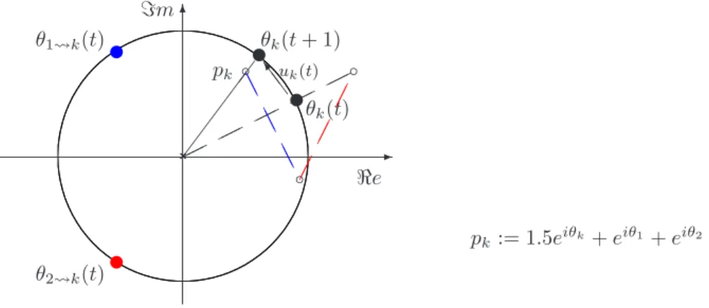
Keywords: Stochastic algorithms, simulated annealing, homogenization, probability mea- sures on compact Riemannian manifolds, intrinsic p-means, instantaneous invariant measures,

Put the verb into the correct form, simple present or preterit, active

In the middle of your page, draw the 6 cm diameter long circle. Mark a point A on this circle and draw

Then draw the perpendicular bisector of segment [SA] : this line cuts line (d’) in point M.. Do it again and again with various points A placed regularly on