Systematic analysis of site-specific yield distributions resulting
from nitrogen management and climatic variability interactions
Benjamin Dumont • Bruno Basso • Vincent Leemans •
Bernard Bodson • Jean-Pierre Destain • Marie-France Destain
Abstract
At the plot level, crop simulation models such as STICS have the potential to evaluate risk associated with management practices. In nitrogen (N) management, however, the decision-making process is complex because the decision has to be taken without any knowledge of future weather conditions. The objective of this paper is to present a general methodology for assessing yield variability linked to climatic uncertainty and variable N rate strategies. The STICS model was coupled with the LARS-Weather Generator. The Pearson system and coefficients were used to characterise the shape of yield distribution. Alternatives to classical statistical tests were proposed for assessing the normality of distributions and conducting comparisons (namely, the Jarque-Bera and Wilcoxon tests, respectively). Finally, the focus was put on the probability risk assessment, which remains a key point within the decision process. The simulation results showed that, based on current N application practice among Belgian farmers (60-60-60 kgN ha-1), yield distribution was very highly significantly non-normal, with the highest degree of asymmetry characterised by a skewness value of -1.02. They showed that this strategy gave the greatest probability (60%) of achieving yields that were superior to the mean (10.5 t ha-1) of the distribution.
Keywords Nitrogen management ∙ Climatic variability ∙ LARS-WG Weather Generator ∙ STICS Soil-crop model ∙ Pearson system ∙ Probability risk assessment
Benjamin Dumont (), Vincent Leemans & Marie-France Destain
ULg Gembloux Agro-Bio Tech, Dpt. Environmental Sciences and Technologies, Precision Agriculture Unit Passage des Déportés, 5030 Gembloux, Belgium
e-mail: [email protected]
Tel.: +32(0)81/62.21.63, fax: +32(0)81/62.21.67 Bruno Basso
Dept. Geological Sciences & W.K. Kellogg Biological Station, Michigan State University, East Lansing, USA Bernard Bodson
ULg Gembloux Agro-Bio Tech, Dept. Agronomical Sciences, 5030 Gembloux, Belgium Jean-Pierre Destain
ULg Gembloux Agro-Bio Tech – Walloon Agricultural Research Centre (CRA-W), 5030 Gembloux, Belgium
1
2
3
4
5
6
7
8
910
11
12
13
14
15
16
17
18
19
20
21
22
2324
25
26
27 28 29 30 31 33 34 36 37 39 40Introduction
Appropriate nitrogen (N) management is one of the primary challenges in agricultural production and related environmental impact. High grain yields are usually obtained when there is high and appropriate N fertilizer application and favourable precipitation (Welsh et al., 2003). When excessive N fertilizer is applied, however, significant N losses can occur from these systems, with significant environmental consequences, including water pollution and greenhouse gas emissions. Nitrogen fertilizer applications to cropping systems can have low use efficiency, with crops taking up between 40 % and 80 % of the N fertilizer added to these systems . The remaining fraction stays in the soils, or leaves the systems via air, surface water or groundwater pathways . Leaving aside soil N sequestration, N losses are due to nitrate leaching, ammonia volatilization and nitrous oxide emissions . Reducing these losses would require a better and more efficient way of selecting optimal N rates. However, determining the optimum amount of N fertilizer to meet plant needs while simultaneously optimizing the economic return and minimizing environmental impacts remains a non-trivial task .
One of the potential issues to improve yield or nitrogen use efficiency by site-specific nitrogen fertilization is to determine the causes of yield variation before fertilization . In depicting the state-of-the-art in precision agriculture, McBratney et al. (2005) highlighted the important research that has been devoted to yield mapping or quantifying soil variation for zone management . However, in the future, to develop the precision agriculture concept to its full potential, the recognition of methods for the assessment of temporal yield variation requires urgent attention by researchers . A promising approach to select the best N management strategies while reducing the economic and environmental risk associated with such selection and dealing with the temporal variations lies in the use of crop models. Crop models are designed to simulate processes in the soil-plant-atmosphere system. They have been proven effective and fundamental to the decision-support tools used to help farmers, agricultural consultants and policy-makers optimize their decisions . Crop simulation models can quantify the interaction between multiple stresses and crop growth under different environmental and management conditions . They have been shown to be useful in the tactical management of N fertilizer rates associated with easily observed variables (such as water availability based on rainfall amounts). Basso et al. (2011a, 2012b) demonstrated the economic and environmental advantages of varying fertilizer amounts over space (different zones within the field) and time (over different years).
Climate plays a crucial role in the accuracy of a model’s outputs (e.g. grain yield) . Most crop models simulate the evolution of the agronomic variables on a day-by-day basis . Weather conditions therefore need to be described as accurately as possible . A methodologically still more consistent approach to study the effects of
1
23
4
5
6
7
8
9
10
11
12
1314
15
16
17
18
19
20
21
22
23
24
25
26
27
2829
30
climatic variability on crop response is to use a stochastic weather generator, instead of historical data, which are often not numerous . Stochastic weather generators are used to produce unlimited synthetic time series of weather data based on the statistical characteristics of observed weather sequences at a given location. In conjunction with a crop simulation model, a stochastic generator will allow the temporal extrapolation of observed weather records in order to assess the agricultural risk linked to the experimental site.
The preliminary requirement for the selection of the best management practice consists in assessing the probability that a certain outcome (e.g. grain yield or N leaching) will occur under determined pedo-climatic conditions and the investigated management practice. On this basis, the main strategy behind the selection of the best practice could be to select the ones that optimise the probabilities of occurrence (e.g. maximising grain yield or minimising N leaching), or that minimise the corresponding variability around a targeted goal. In the context of precision farming, considering that the pedological conditions are determined by the field and that all other managements practices are imposed by the farmers (e.g. sowing date, irrigation), the complexity of decision-making in terms of N management scenarios is linked to the unknown future weather conditions. A feasible approach for coping with this is to quantify the uncertainty associated with various historical weather scenarios . Based on long-term historical weather data, it has been demonstrated how crop models could be used to develop strategic management practices that optimise N use efficiency, yield and environmental impact, without any knowledge of future weather conditions being required .
As it is the best way to quantify the probabilities of occurrence, defining the most appropriate type of yield distribution observed at the field or plot scale is thus another important parameter to consider when selecting management strategies. A wide variety of methods have been used to determine types of yield distributions based on observed data from field experiments (Day, 1965; Du et al., 2012; Hennessy, 2009a, b; Just and Weninger, 1999). Day (1965) stated that crop yields have a finite lower limit in their range, namely 0. Clearly, the yields could never be negative, but in particular conditions (e.g. an extremely cold winter), yield could be drastically decreased. There is also evidence that a given crop variety has a finite upper limit which, under constant management practices but variable weather conditions, could be limited to a maximum amount, even under the most favourable circumstances, which value is known as the yield potential. Referring to the Pearson's coefficients to analyse and quantify the probabilities within yield distribution functions, Day (1965) demonstrated that the skewness (degree of asymmetry) and kurtosis (degree of flattening) of yield distributions were found to depend upon the specific crop and the amount of available nutrients. Proceeding to similar analysis of yield distributions, Du et al. (2012), concluded that the development of a complete theory on how input constraints affect yield skewness will need much more empirical evidence. Such a research would indeed 1
2
3
4
5
67
8
9
10
11
12
13
14
15
16
17
1819
20
21
22
23
24
25
26
27
28
29
30
31
require extensive experiments where diverse crops should be grown in various production environments and over multiple seasons. However, recent preliminary work has demonstrated that these issues could be overcome by the concomitant use of crop models and stochastic weather generators .
The objective of this research was to evaluate the simulated crop response of a winter wheat cultivar (Triticum aestivum L.) under different N management strategies and stochastically generated climatic data. The way that input constraints affected the simulated yield distributions within the context of the Pearson system was also studied and discussed to refine the guidelines in terms of N management on the specific site of the case study.
Materials and methods
Description of the experimental case study
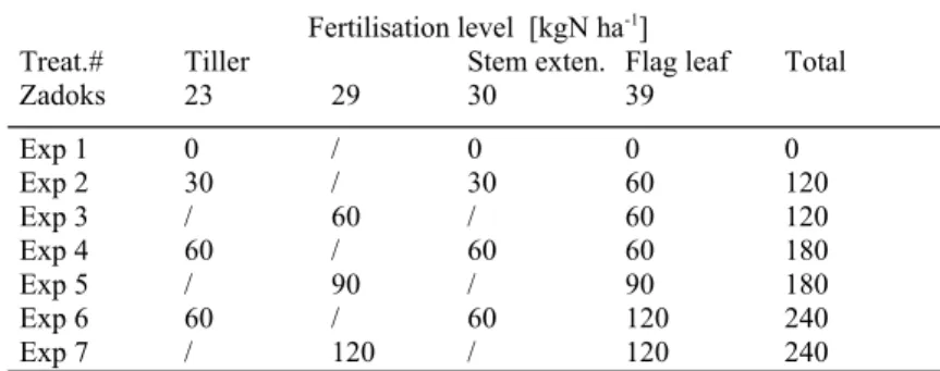
Between 2008 and 2011, a field experiment was designed to study, over the whole season, the growth of a wheat cultivar (Triticum aestivum L., cv. Julius) in the agro-environmental conditions of the Hesbaye region in Belgium under variable N management practices. Seven N fertilisation strategies were analysed, with different rates and timing of fertilizer being applied, as described in Table 1. The experimental N strategies were designed around the Belgian farmers' current practice, which consists of applying 60 kgN ha-1 respectively at tiller (Zadoks 23), stem extension (Zadoks 30) and flag leaf stages (Zadoks 39) (Zadoks et al, 1974), and represented under the experimental treatment number 4 in Table 1. The cultivar was sown between October and mid-November and usually harvested between very late July and mid-August.
The measurements considered for the simulation purpose were the results of four repetitions by date, nitrogen level and crop season. Each repetition was performed on a small block (2 m × 6 m) and the blocks were implemented on a classic loam soil type according to a complete randomised block distribution to ensure measurement independence. During this experiment, biomass (total dry matter and grain yield), plant N uptake and soil N content were measured at regular intervals during the growing seasons and at harvest. The measurements were performed over the three successive crop seasons (2008-09, 2009-10 and 2010-11). The above-ground biomass measurements were collected at bi-weekly intervals from mid-February until harvest. The measurements were carried out on dried samples, corresponding to the sampling of three adjacent 500 mm rows separated from 146 mm. After anthesis stage, the above-ground biomass accumulation was defined separately for straw and grain. Once per month, the biomass samples were crushed and their N content was analysed using the Kjeldahl method. Once every two weeks, alternating with the sampling of biomass, the soil N contents were 1
2
3
45
6
7
8
9
10
1112
13
14
15
16
17
18
1920
21
22
23
24
25
26
27
28
29
measured in 150mm soil layers. As they are time- and money-consuming, these measurements were only performed under the experimental plot corresponding to the application of 60-60-60 kgN ha-1 (Exp 4 in table 1) as this treatment corresponded to the most usual N strategy as practiced by farmers.
Table 1 Details of the field trials to study the crop response to variable N management, where different amounts and timing of N applications were investigated.
Fertilisation level [kgN ha-1]
Treat.# Tiller Stem exten. Flag leaf Total
Zadoks 23 29 30 39 Exp 1 0 / 0 0 0 Exp 2 30 / 30 60 120 Exp 3 / 60 / 60 120 Exp 4 60 / 60 60 180 Exp 5 / 90 / 90 180 Exp 6 60 / 60 120 240 Exp 7 / 120 / 120 240
Crop model description, calibration and validation
The STICS crop growth model (STICS V6.9) used in this study has been described in several papers . It simulates the water, carbon and N dynamics in the soil-plant-atmosphere system on a day-by-day basis. It allows the effect of water and nutrient stress on development rate to be taken into account. It requires daily weather data inputs (i.e. minimum and maximum temperatures, total radiation and total rainfall, vapour pressure and wind speed).
The STICS model parameterisation, calibration and validation were performed on the 3-year database described in the field trial described in the previous section. Regularly used in crop modelling, root mean square error (RMSE), Nash-Sutcliffe Efficiency (NSE) and normalised deviation (ND) were used to judge the quality of the model (Table 2) . The calibration process was performed using the DREAM(-ZS) Bayesian algorithm .
Parameters involved in the phenology (stlevamf, stamflax), the leaf area development (adens, dlaimaxbrut, durvieF), parameters directly related to biomass growth (efcroijuv, efcroirepro, efcroiveg), grain filling (cgrain, irmax) and finally related to water and nitrogen stresses (psisturg, psisto, INNmin) were optimised. The remaining parameters of the species were fixed at the suggested default values (Brisson et al., 1998; 2003).
The parameters were calibrated on the results obtained under the treatments Exp1 and Exp4 of the field trial (Table 1) for the three crop seasons 2008-09, 2009-10 and 2010-11. The model was then validated on all the other treatments (Exp 2, Exp 3, Exp 5, Exp 6 and Exp 7 of Table 1) for all crop seasons. The parameters were 1
2
3
4 56
7
8
910
11
12
13
1415
16
17
1819
20
21
22
2324
25
optimised to correctly simulate the biomass growth and grain yield, on which this paper focuses, but also the plant N uptake, which is intrinsically linked to biomass growth. As the soil N measurements were only available under the Exp 4, the data were only used to control that the dynamic nature of nitrogen in the soil was correctly represented, but they were not directly used to optimise parameters.
As recommended by Guillaume et al. (2011), a single-step calibration procedure - involving all the output variables (i.e. the total biomass, the grain yield and the plant N uptake over the three cropping seasons) and all the parameters to optimize - was used instead of a multiple-step optimization procedure. This ensured avoiding the over-parameterization phenomena (Dumont et al., 2014b).
More detail about the procedure and the results obtained can be found in Dumont et al. (2014b).
Assessing nitrogen management strategy
Two sets of N practices, that differed in terms of N amount and/or timing, were analysed. (Table 2). A total of 19 N strategies, described below, were evaluated. The first set of N applications was based on supplying the total N amount in three equal fractions, applied at the tillering (Zadoks 23), stem extension (Zadoks 30) and flag-leaf (Zadoks 39) stages. The practices differed by an increase of 10 kgN ha-1 per application, ranging from 0 kgN ha-1 to 300 kgN ha-1 for the total N application (3×100 kgN ha-1).
The second set of N practices was based on supplying the N in two equal fractions. The first application was made at an intermediary stage between tiller and stem extension stage (Zadoks 29) and flag leaf stage (Zadoks 30). An increasing step of 15 kgN ha-1 per application was simulated, ranging from 0 kgN ha-1 to 240 kgN ha-1 (2×120 kgN ha-1).
Applying the N in two fractions instead of three may be suitable for different reasons. If wheat is involved in rotation or if trap crops are part of the cropping system, the soil may not be totally depleted in nitrogen at wheat sowing, which could allow modification of N timing of the first application. On the other hand, applying nitrogen in two equal fractions may be useful for limiting the number of field interventions, thus reducing fuel consumption. It is also worth mentioning that, in Belgium, splitting the N application in two doses is a current practice, notably recommended if the preceding culture is a potato, rapeseed or a leguminous crop. Table 2 Fertilisation calendar for the variable N practices (two and three fractions) evaluated using the crop model simulations. 1
2
3
4
56
7
8
910
1112
13
14
15
1617
18
19
2021
22
23
24
25
2627
Fertilisation calendar (according to Zadoks stage and Julian day) Tiller Stem exten. Flagleaf
Zadoks 23 29 30 39
Julian day 445 460 475 508 Fertilisation rate [kgN ha-1]
Treat.# Tiller Stem exten. Flagleaf Total
T1 0 / 0 0 0 T2 10 / 10 10 30 T3 20 / 20 20 60 T4 30 / 30 30 90 ... ... ... ... ... ... T11 100 / 100 100 300 T1 / 0 / 0 0 T12 / 15 / 15 30 T13 / 30 / 30 60 T14 / 45 / 45 90 ... ... ... ... ... ... T19 / 120 / 120 240
Weather database, weather generator and climate variability
The historical weather records on solar radiation, precipitation and temperatures were provided by the Ernage weather station, which is part of Belgium’s Royal Meteorological Institute (RMI) observation network (http://b-cgms.cra.wallonie.be/). The Ernage station is located 2 km from the experimental field. The complete 31-year (1980-2011) weather database (WDB) was used in this study in order to provide the inputs for the crop model.
The Ernage WDB was analysed using the LARS-Weather Generator (WG) , which computed a set of parameters representing the experimental site. The characteristic value of the weather time series are the daily maximum, minimum, mean and standard deviation values of each climatic variable, the frequency distributions of rain, and the seasonal frequency distributions for wet and dry series.
The LARS-WG was then used to generate a set of stochastic synthetic weather time-series representative of the climatic conditions in the area. As defined by Semenov and Barrow (2002), one of the properties of the LARS-WG is that it can be used "to generate synthetic data which have the same statistical characteristics as the observed weather data" . The statistical parameters derived from the observed weather data are directly used by LARS-WG : the synthetic weather data will thus be different on a day-to-day basis, and over the simulated years, although the statistical characteristics will remain the same as the historical record. As advocated by Semenov and Barrow (2002), long weather sequences are usually required for risk assessment as the longer the time period of simulated weather used, the more they cover the range of possible weather events.
Lawless and Semenov (2005) demonstrated that a set of 60 synthetic weather time-series was enough to
1
2
34
5
6
7
89
10
11
1213
14
15
16
17
18
19
20achieve stability in predicted mean grain yield. However, as the stochastic component of LARS-WG is driven by a random seed number, Lawless and Semenov (2005) recommended using at least 300 stochastically generated weather time-series. The same number of stochastically-generated climates were used in this study.
The stochastically-generated climatic set could then be input into the STICS crop model. Proceeding in such a way ensures the exploration of new combinations of weather variables, which can lead to simulated stresss conditions that have not previously been observed within the field, but that responded to local climatic conditions.
Statistical consideration
In this research, as distribution describers, the Pearson system and coefficients were used to finely characterise the shape of yield distributions. Furthermore, in order to evaluate and compare the impact of the different N strategies, different statistical tests were deployed. As alternatives to the usual Kolmogorov-Smirnov and ANOVA tests usually referenced in the literature and respectively used to evaluate the normality and to assess the equivalence of distributions, this paper proposed two other tests, namely the Jarque-Bera and Wilcoxon tests.
The Pearson type I distribution
Pearson developed an alternative system of density functions that takes a wide variety of forms . The Pearson system of density function is derived from the differential equation:
( ) ² 2 1 0 x f x c x c c a x dx x df (1) in which x is the random variable and f(x) its density function. Through the integrals of this equation, the constants a, c0, c1, c2, allow the different types of distribution in the Pearson system to be characterised.In this paper, the focus was put on Type I distribution, for which the random variable has a finite range:
y or y y x x k x f m m 2 1 2 1 2 2 1 1 , 0 , ) ( ) .(
(2) where α1 and α2 are the roots of the quadratic term in Eq. 1, and m1 and m2 are the coefficients of shape. Type I distribution is also known as Beta distribution.The Pearson coefficients
One advantage of the Pearson system is that the different types of distribution can be identified independently from their means and variances, but rather referring to two coefficients of shape, namely their skewness and 1
2
3
45
6
7
8
910
11
12
13
14
1516
17
1819
2021
2223
24
2526
kurtosis parameters. Pearson therefore defined the β1 and β2 parameters thus: 4 4 2 2 4 2 6 2 3 3 2 2 3 1
m
m
m
m
m
m
(3) where mp is the mean-centred moment of order p, defined according to the mean value Sn/n, and computed as:
n i p n i pn
S
X
n
m
11
(4)The β1 parameter is known as the squared skewness, which is defined as the 3rd moment divided by the cube of the variance. The β2 parameter is known as the kurtosis.
Following Pearson , the existence range of the β1 and β2 parameters can be used to represent the two axes of a real plane. The plane is subdivided in zones delimited by characteristic reference values of β1 and β2. Each zone of this space makes reference to a particular distribution type of the Pearson's system. For any given experimental distribution, the nominal β1 and β2 parameters can be computed. Their values can then be (graphically) compared to the reference values which allows the type of function that best represents the experimental sampling to be determined.
Assessing the normality of distributions
The one-sample Kolmogorov-Smirnov (KS) test compares the values in a data vector with the standard normal distribution in order to see if the two datasets differ significantly. The KS test requires reducing the data vector by its mean and normalising it by its standard deviation.
The Jarque-Bera (JB) test is an alternative way of assessing the normality of distributed random variables, and is specifically designed for alternatives in the Pearson system. In contrast to the KS test, the JB test does not rely on knowing the mean, but rather on the skewness and kurtosis, and is therefore more related to the shape of the distribution. Moreover, the JB test is particularly suited for large samples of data (ideally > 100) which requirement was largely found with the 300 synthetic weather realisations.
Assessing the equivalence of the distributions
The purpose of one-way ANOVA is to find out whether data from several groups have a common mean. The ANOVA test determines whether the groups are actually different in the measured characteristic. It relies on the 1
2
34
5 67
89
10
11
12
13
14
1516
17
1819
20
21
22
23
2425
assumption that the data in the vector of the samples are (i) normally distributed, (ii) have equal variance and (iii) are mutually independent.
The Wilcoxon test can be used to compare, in pairs, the medians of the distributions obtained under the various N treatments. This test assesses whether data in each of two evaluated vectors are independent samples from identical continuous distributions, or, equivalently, from different populations with the same distribution, with equal medians. Regarding the hypothesis on which the ANOVA test relies, the Wilcoxon test should be preferred when distributions are found to be non-normal.
Simulation process, conditions of application of the method and N strategies evaluation
For the purpose of this study, it was assumed that cultivar, soil and management techniques (other than N practices) remained the same for all simulations. Therefore the simulations carried out differed only in their weather inputs. Such practice is of common use in crop modelling and allows easier interpretation and comparison of the model outputs. Furthermore, in the context of precision agriculture, proceeding in that way responds to a concrete need : with the availability of new varieties on the market or the emergence of new environmental directives, farmers may be interested to know if the usual N recommendations would still be the most adapted under any local condition and the upcoming probable weather conditions. Being generic, the methodology described in this paper can be easily applied to any other initial soil conditions or management practices (e.g. sowing date).
Therefore, in accordance with agronomists, a management itinerary determined as a conventional itinerary was applied to each simulation. The sowing date was in late October, on Julian day 295. Each simulation was run with the sowing date as the starting point. The same soil description was used for all simulations. The soil-water content was initiated at field capacity, which was a reasonable assumption according to the usual pluviometry at this time of year in Belgium. The soil initial inorganic N content corresponded to the measurements conducted in 2008-09 and presented as a case study; as the crops sown in 2008-09 were included in a rotation, these measurements were considered representative of the real-life conditions.
Grain yield values for the 300 climatic projections were computed in a vector. The mean, standard deviation, β1 and β2 values of each distribution were then calculated. The β1 and β2 values are also used to calculate the c0, c1 and c2 parameters. These values are automatically compared with the abacus developed by Pearson in order to identify the distribution type. Knowing these parameters allows the theoretical corresponding function to be generated using the Matlab ‘pearsrnd’ function. It is important to mention that the theoretical Pearson distribution thus generated is not a fitted function, but rather a computed function of the characteristics 1
2
34
5
6
7
8
910
11
12
13
14
15
16
17
1819
20
21
22
23
24
2526
27
28
29
30
value. One can here speak of an adjustment by the method of moments. The theoretical distribution can then be compared with the numerical-experimental results.
Software
The data analysis and treatment were done using Matlab software and toolboxes (Matlab, Mathworks Inc., Natick, Massachusetts, USA).
Results
Simulation of the experimental case study
In 2008-2009, the experimental yields obtained were fairly high, close to the optimum for the cultivar. This was due mainly to good weather conditions and adequate N rates. The season 2009-10 was characterised by a significant water stress that occurred early in the season (February) and in the early summer (July) leading to yield losses. Furthermore, poor summer conditions delayed the grain filling period and harvest time. In 2010-11, water stresses occurred from February until the end of May, with only 80mm of precipitation in four months. In the summer, rainfall returned and there was correct filling of the grains, resulting in a good grain yield. However, straws remained very short and straw yield remained low. Under no application of nitrogen (Exp1 - Table 1), the mean observed yields equalled 9.2, 4.7 and 4.8 t ha-1, respectively for the crop seasons 2008-09, 2009-10 and 2010-11. Where 60-60-60 kgN ha-1 were applied (Exp4 - Table 1), the observations were respectively equalling 12.3, 7.8 and 7.4 t ha-1 for the same years.
The usual threshold expected in crop modelling for NSE (NSE > 0.5) was largely met during the calibration and validation steps for biomass, grain yield and plant N uptake (Table 3). A slight deviation was observed for the ND criteria (|ND|<0.1-0.15) obtained at grain yield validation. They resulted from the data collected during the crop season 2010-11, which was known to be particularly challenging in terms of modelling, since deep water deficits occurred.
Concerning the process linked to N dynamics, the STICS model simulated particularly well the plant N uptake, with very good NSE and ND criteria, both in calibration and validation phases While the RMSE and ND criteria of soil N content were reasonable over the simulated soil profile (0-1500 mm), the corresponding NSE was however characterised by a negative value.
Table 3 Results of the model evaluation on the three contrasted crop seasons and the seven N protocols 1
2
3
45
6
7
89
10
11
12
13
14
15
16
17
1819
20
21
22
2324
25
26
27CALIBRATION VALIDATION
Variable RMSE NSE ND RMSE NSE ND
[unit] [/] [/] [unit] [/] [/] Biomass [t ha-1] 2.15 0.84 0.15 2.27 0.84 0.16
Grain yield [t ha-1] 1.49 0.76 0.19 1.81 0.69 0.23
Plant N uptake [kgN ha-1] 30.39 0.78 0.14 36.31 0.63 0.09
Soil N content [kgN ha-1] 11.09 -0.75 -0.03 / / /
As an illustration, Fig. 1 shows the simulations of the total biomass, grain yield, plant N uptake and N-NO3- content in the upper soil layer (0-300 mm). The results focused on the crop season 2009-10 for winter wheat growing under the N strategy where the farmer's current practice was applied (Exp 4 of the case study -Table 1). As can be seen, the simulation of the total biomass and grain yield were properly reproduced by the model. While the NSE criterion was not particularly good, the global dynamics of N in the soil were however correctly simulated, especially each time N was applied. The corresponding dynamics of N exported by the plant were also accurately simulated.
1
23
4
5
6
7
8
9
Fig. 1 Observations (black dots) and simulations (solid black line) of the total biomass, grain yield, plant N uptake and mineral N-NO3- content in the upper soil layer (0-300 mm) for the crop season 2009-10 under the Exp 4 (60-60-60kgN ha-1) of the case study.
Simulation of yield response to N practices
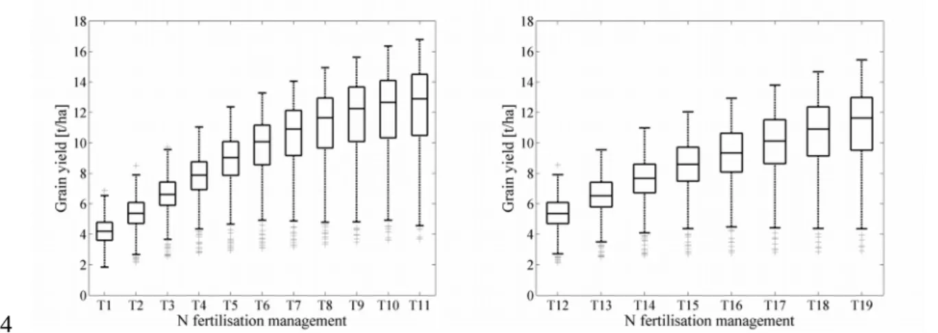
The grain yields simulated for the 300 stochastic climate conditions are shown as boxplots in Fig. 2, with N management strategies based on two and three fractions. Initially, the N strategies were compared within each group. Each increase in N amount led to higher median and maximal yields. However, provided a total of at least 90 kgN ha-1 (T4 to T11 and T14 to T19) was applied to the crop, a relatively constant minimal yield of 3 t ha-1 was achieved. A comparison of the two graphs in Fig. 2 showed a systematic higher median value in the three fractions protocol on the two fractions ones, for the same level of fertilisation.
Fig. 2 Boxplot analysis of the grain yields corresponding to the various N fertilization strategies investigated with the crop model
1
34
5
6
7
89
10
11
12
13
14
1516
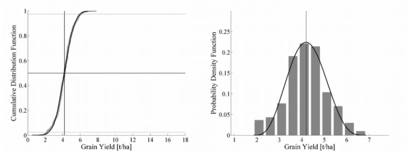
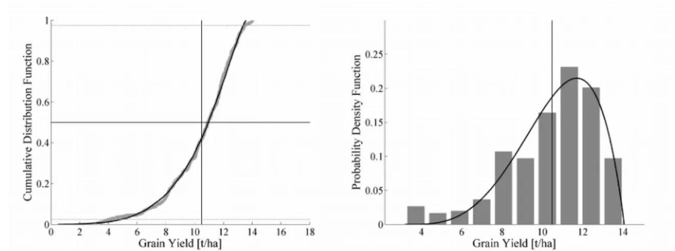
17Fig. 3 presents three specific levels: 0-0-0 kgN ha-1 (T1); 60-60-60 kgN ha-1 (T7); and 100-100-100 kgN ha-1 (T11). For these levels, both the cumulative distribution function (CDF) and the probability density function (PDF) are presented. In each case, the computed theoretical function (solid black lines) matched the numerical-experimental distribution (solid grey lines or grey histograms) very accurately. The computed Type I distribution therefore seemed particularly suited for representing the crop model response. The simulated yield distributions were consistent with the in-field experiments conducted to calibrate the model (cf previous section).
It was also observed that the grain yield distribution under the T1 treatment exhibited a close-to-normal distribution. Each additional N supply led to an increase in the simulated yield, i.e. characterised by a right displacement of the mean and the median. At the same time, a negative skewness was observed, translated by a median value superior to the mean. This effect was illustrated in the CDF graphs. Thus, a negative skewness increased the probability of obtaining a final yield higher than the mean of the distribution. Therefore, supplying N to the crop increased both the expected grain yield and the probability of achieving a yield higher than the mean of the distribution.
1
2
3
4
5
6
78
9
10
11
12
13
1415
Fig. 3 Cumulative distribution function (CDF) and probability density function (PDF) corresponding to the T1 top), T7 (middle) and T11 (lower) treatments (i.e. the '0-0-0', '60-60-60' and '100-100-100' N management strategies, respectively). Comparison of the numerical-experimental curve (grey line) and the computed Type I distribution of the Pearson system (black line). The left graph also shows the 50 percentile (solid horizontal thick black line) and the 2.5 and 97.5 percentiles (dashed horizontal thick grey line). The vertical black line represents the mean of the distribution.
1
2
34
5
6
7
8
9Analysis of the skewness and kurtosis of the distribution
The skewness and kurtosis parameters of each N management strategy are presented in Fig. 4. These parameters evolved in opposite directions: when the dissymmetry was more pronounced, the curve was more spread. This was a consequence of the lowest yields, which were constant at about 3 t ha-1, whereas the highest yields increased with N management.
The three-fraction N management strategy gave the highest degree of asymmetry, with a skewness value of -1.02 for the 60-60-60 kgN ha-1 treatment (T7). The asymmetry decreased a little after that, reaching -0.83 at 100-100-100 kgN ha-1 (T11). The non-application of N (T1) resulted in a distribution with close-to-zero skewness (-0.002) and a kurtosis close to 3. These values were very similar to the Gaussian distribution, for which skewness and kurtosis were 0 and 3, respectively. The skewness values obtained with the two-fraction N management strategy ranged between -0.32 and -0.84, where some asymptote was reached.
1
23
4
5
67
8
9
10
11
1213
Fig. 4 Skewness and kurtosis of the grain yield distributions corresponding to the various N fertilisation strategies investigated with the crop model
Assessing the normality
This section focuses on the comparison of both KS and JB test results, respectively presented in Table 4 and Table 5. Using a KS test, the three-fraction N management strategy showed the distribution to be normal up to a treatment of 10-10-10 kgN ha-1. The two-fraction N management strategy resulted in normal behaviour under N inputs up to 75-75 kgN ha-1.
Table 2 Assessing the normality using the Kolmogorov-Smirnov (KS) test
Treat. 0-0-0 10-10-10 20-20-20 30-30-30 40-40-40 50-50-50 60-60-60 70-70-70 80-80-80 90-90-90 100-100-100 p-value 0.766 0.338 0.023* 0.017* 0.018* 0.013* 0.007** 0.006** 0.002** 0.004** 0.003** Treat. 0-0 15-15 30-30 45-45 60-60 75-75 90-90 105-105 120-120
p-value 0.766 0.249 0.056 0.057 0.055 0.064 0.023* 0.003** 0.007**
Table 3 Assessing the normality using the Jarque-Bera (JB) test
Treat. 0-0-0 10-10-10 20-20-20 30-30-30 40-40-40 50-50-50 60-60-60 70-70-70 80-80-80 90-90-90 100-100-100 p-value 0.500 0.059 0.003** 0.001*** 0.001*** 0.001*** 0.001*** 0.001*** 0.001*** 0.001*** 0.001*** Treat. 0-0 15-15 30-30 45-45 60-60 75-75 90-90 105-105 120-120
p-value 0. 500 0.066 0.004** 0.001*** 0.001*** 0.001*** 0.001*** 0.001*** 0.001***
Under the three-fraction strategies, the same conclusion as obtained with the KS test were drawn when the JB test was used; the distributions could be considered as being not different from normal distribution only up to 30 kgN ha-1 application (10-10-10 kgN ha-1). The results differed significantly for the two-dose splitting protocols. Since 30-30 kgN ha-1 fertiliser were applied, the corresponding distributions were found to be non-normal. It was also notable that the p-value obtained was systematically far lower with the JB test than with the
1
23
4
5
67
8
9
10 11 12 13 1415
16
17
18
KS test. These results highlighted the importance of considering the shape of a distribution, through its skewness and kurtosis, when its normality had to be assessed.
Comparison of the N management strategies
The ANOVA test is known to be robust with respect to small deviations from the first two assumptions on which it relies. However, as the JB test performed earlier showed that the data vector were mostly highly significantly non-normal ('***'), only the Wilcoxon test was performed in this study. The results of the Wilcoxon test are presented at Tables 6, 7 and 8.
Overall, each additional N application led to at least a significant ('*') increase of the mean of the grain yield distribution (Tables 6 and 7), whatever N was provided in two or three fractions. Under the N management strategies where the applications were of 90-90-90 and 100-100-100 kgN ha-1, the distributions were judged as having a non-significant difference in their median. The same conclusions would probably have been reached with higher two-fraction N strategies.
Table 4 Comparison of N treatments in the three-fraction N management strategy, using the Wilcoxon test, based on comparing pairs of treatments
Treat. 100-100-100 90-90-90 80-80-80 70-70-70 60-60-60 50-50-50 40-40-40 30-30-30 20-20-20 10-10-10 90-90-90 0.145 80-80-80 0.000*** 0.030* 70-70-70 0.000*** 0.000*** 0.002** 60-60-60 0.000*** 0.000*** 0.000*** 0.000*** 50-50-50 0.000*** 0.000*** 0.000*** 0.000*** 0.000*** 40-40-40 0.000*** 0.000*** 0.000*** 0.000*** 0.000*** 0.000*** 30-30-30 0.000*** 0.000*** 0.000*** 0.000*** 0.000*** 0.000*** 0.000*** 20-20-20 0.000*** 0.000*** 0.000*** 0.000*** 0.000*** 0.000*** 0.000*** 0.000*** 10-10-10 0.000*** 0.000*** 0.000*** 0.000*** 0.000*** 0.000*** 0.000*** 0.000*** 0.000*** 0-0-0 0.000*** 0.000*** 0.000*** 0.000*** 0.000*** 0.000*** 0.000*** 0.000*** 0.000*** 0.000***
Table 5 Comparison of N treatments in the two-fraction N management strategy, using the Wilcoxon test, based on comparing pairs of treatments
Treat. 120-120 105-105 90-90 75-75 60-60 45-45 30-30 105-105 0.002** 90-90 0.000*** 0.000*** 75-75 0.000*** 0.000*** 0.000*** 60-60 0.000*** 0.000*** 0.000*** 0.000*** 45-45 0.000*** 0.000*** 0.000*** 0.000*** 0.000*** 30-30 0.000*** 0.000*** 0.000*** 0.000*** 0.000*** 0.000*** 15-15 0.000*** 0.000*** 0.000*** 0.000*** 0.000*** 0.000*** 0.000***
Table 6 Comparison of N management strategies based on two- and three-fraction treatments, using the Wilcoxon test. Treat. 120-120 105-105 90-90 75-75 60-60 45-45 30-30 15-15 1
2
3
45
6
7
89
10
11
12
1314
15 1617
18 1920
80-80-80 0.001*** 0.000*** 0.000*** 0.000*** 0.000*** 0.000*** 0.000*** 0.000*** 70-70-70 0.643 0.000*** 0.000*** 0.000*** 0.000*** 0.000*** 0.000*** 0.000*** 60-60-60 0.000*** 0.773 0.000*** 0.000*** 0.000*** 0.000*** 0.000*** 0.000*** 50-50-50 0.000*** 0.000*** 0.176 0.001*** 0.000*** 0.000*** 0.000*** 0.000*** 40-40-40 0.000*** 0.000*** 0.000*** 0.003** 0.009** 0.000*** 0.000*** 0.000*** 30-30-30 0.000*** 0.000*** 0.000*** 0.000*** 0.000*** 0.123 0.000*** 0.000*** 20-20-20 0.000*** 0.000*** 0.000*** 0.000*** 0.000*** 0.000*** 0.612 0.000*** 10-10-10 0.000*** 0.000*** 0.000*** 0.000*** 0.000*** 0.000*** 0.000*** 0.892
Table 8 presents the results of the Wilcoxon test conducted to compare the two- and three-fraction N management strategies. From 0 to 90 kgN ha-1 (either 30-30-30 or 45-45 kgN ha-1), the strategies with the same total N application were non-significantly different. In terms of total N amount applied, each increase of 3 x 10 kgN ha-1 was equivalent to an increase of 15 kgN ha-1 applied in two fractions. There was a transient zone between the 120 and 150 total N applications. With the higher N protocols, the median of the three-fraction strategy was equivalent to the median of the two-fraction strategy that required 30 kgN ha-1 more. This clearly demonstrated the superiority of the three-fraction strategy in achieving higher yields. The corollary effect was that 30 kgN ha-1 could systematically be saved by splitting the N amount into three applications when more than 150 kgN ha-1 had to be applied over the season.
Probability risk assessment
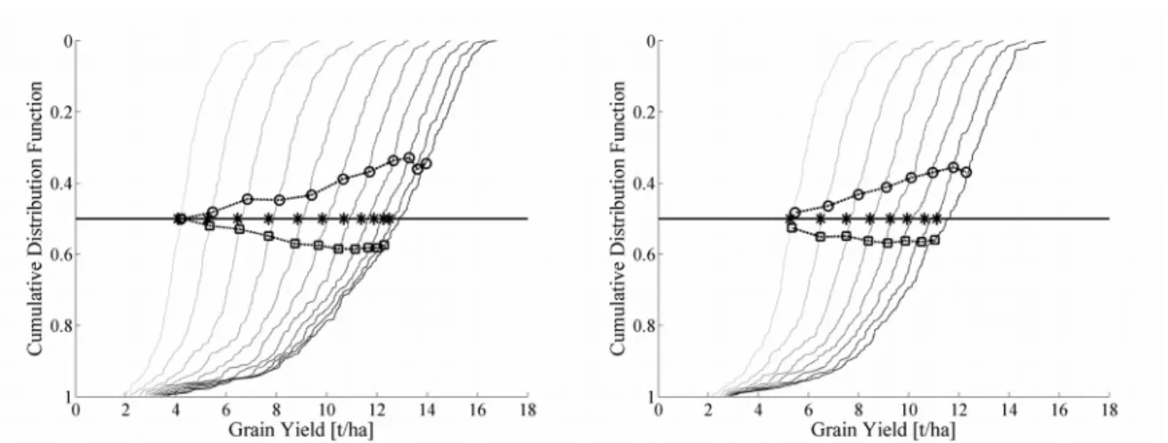
Fig. 5 provides the model grain yield result as a function of N fertilisation management and cumulative probability density function (CDF) drawn out of 300 synthetic climate realisations. The y-axis was inverted, in order to correspond to the risk for the farmer to achieve the expected corresponding yield. The increasing N treatments were represented by the darkening grey line. The characteristics values, namely the mean, the median and the mode of each distribution were numerically derived and overlaid on the response curves.
Fig. 5 Grain yield as a function of N fertilisation management (darkening grey lines) and cumulative probability density function (CDF) drawn out of 300 synthetic climates. The left graph shows the N treatments in three 1 2
3
4
5
6
7
8
9
10
11
1213
14
15
16
17
1819
fractions (from T1 to T11) and the right graph shows the N treatments in two fractions (from T12 to T19). The dotted circled (-o-) lines (upper line) represent the modes of the distributions. The dotted star (-*-) line (intermediate horizontal line) represents the medians of the distributions. The dotted squared (-□-) lines (lower line) represent the means of the distributions.
In this form, one could clearly see how the distributions evolved from Gaussian at low N strategies (0-0-0, 10-10-10 and 15-15 kgN ha-1 protocols), towards an asymmetric shape. Under low N strategies, the mode, the median and the mean were confounded, while they diverged with increasing N practices. Under this representation, with increasing N dose, a shortening distance between the probability curves was clearly noticeable, i.e. a reduced increasing gain of yield with the increase of N level.
With N increase, the probability to achieve at least the mean yield and the mode of the distribution respectively increased and decreased. Under the three-fractions N protocols, the probability to achieve at least the mean yield of the distribution evolved from 50% at the non-application of N (Gaussian distribution) till a bit less than 60% at 60-60-60 kgN ha-1 and higher practices (57.5-58.5%). The chances for the farmer to achieve at least the mean yield were therefore increased by 8%. However, at the same time, the probability of achieving at least the mode decreased from treatment to treatment. It evolved from 50% under no nitrogen application to around 35% at 70-70-70 kgN ha-1 and higher practices. At high N practices, the distance between the mode and the median was always superior to the difference between the median and the mean. When practicing fertilisation in two fractions, the results followed the same tendencies : the highest probability (56.2%) of achieving at least the mean yield was reached at 60-60 kgN ha-1, while the lowest probability to achieve at least the mode was of 35.5% magnitude and was reached under a 105-105 kgN ha-1 protocol.
Discussion
On the necessity to correctly calibrate the model
It is worth remembering that the results offered by the proposed methodology are clearly site-specific : the STICS model was recalibrated for the specific cultivar sown and run on local soil conditions. The climatic inputs of the models were stochastically generated on the basis of characteristic values obtained on a recorded historical database. For such reasons, the simulated model outputs are clearly representative of the local agro-pedo-meteorological conditions.
Furthermore, before any generalisation of the site-specific results over cropping seasons, other 1
2
3
4
5
67
8
9
10
1112
13
14
15
16
17
18
19
20
21
22
23
2425
26
27
28
29simulations carried out with variable initial soil N status should be performed. But, considering that (i) the simulated loam soil is typical of the Hesbaye Region (240000 ha in Belgium),
(ii) the cultivar has characteristics similar to other varieties sown in the area, (iii) the initial soil N values are representative of Belgian farmer's cropping systems,
the results discussed here are general, to some extent, to Belgian farmers’ N management. Finally, the model can be run on variable soil characteristics, variable soil initial N or water conditions, which makes the methodology relevant for precision agriculture purposes.
When too few data are available or too similar experimental conditions are encountered, the major limitation of the calibration process is that it reduces the modelling exercise to an empirical fit of observations under a particular set of circumstances . Performing a calibration of the model on highly contrasted conditions, both in terms of driving inputs or management practices, should thus allow this limitation to be overcome. The selected experimental cases used for the calibration purpose were thus selected to be highly contrasted in terms of N management (0 and 180 kgN ha-1) which made the calibration process challenging, but necessary to adapt the model to the simulation of any N scenarios other than the ones met during field experiments (Table 3). Furthermore, it was decided to use the three available crop seasons to calibrate the wheat climatic response. The crop season 2010-11 was indeed known to be particularly challenging in terms of modelling, since deep water deficits occurred. Once again, it was driven by the necessity to increase the relevance of the calibration process since the model was run on stochastically generated climate conditions which explored disadvantageous climate variable combination.
In the end, the model performances obtained for the STICS model were of very high quality for the simulation of the aerial growth and plant N uptake. They were of similar magnitude as the one obtained by Constantin et al. (2012), who used the same model version, also on temperate climatic conditions. As reported by these authors, and highlighted by a negative efficiency, the variability of soil mineral N was also less well simulated in this case. However, the global dynamics of N in the soil were correctly reproduced.
Improving N recommendation by performing crop model-based probability risk assessment
First, it is worth highlighting that Type I distributions were not fitted to the experimental distribution, but instead were computed on the particular characteristic values of the numerical-experimental distribution, namely the mean, standard deviation, skewness and kurtosis. Over all, the results demonstrated that the Type I distribution of the Pearson system was clearly appropriate for characterising the global model behaviour, under any given N protocol. Since the work of Day (1965) on oats response to variable N rates, this function is known to be a good 1 2 3 4 5
6
7
89
10
11
12
13
14
15
16
17
18
19
2021
22
23
24
25
2627
28
29
30
estimator of experimental crop yield distributions. But it was here transferred for the first time to the analysis of crop model responses.
Some remarks need also to be made with regard to evaluating the normality of the distributions. By reducing and normalising the distribution, the widely used KS test resulted in a slight smoothing of the curve. As an alternative, the JB test was applied for evaluating the normality of the distributions . The JB test might result in a rejection of a hypothesis of normality where a KS test might result in an accept. For this reason, the skewness and kurtosis of distributions are very important parameters to consider when evaluating the normality of distributions, as previously highlighted by Hennessy (2009a). That argues in favour of systematically considering the first four moments of a distribution rather than exclusively the two first (mean and standard deviation) as usually done.
With regard to Figs. 2, 3 and 4, the increasing N strategies had an effect that was expressed in two phases. Under no-application of N, the yield distributions were normal, which corroborated the observations of Day (1965). The law of the minimum was most likely applicable : bad weather conditions resulted in the lowest yield, whereas the lack of N resulted in a limitation to the highest yield. Applying N induced asymmetry in the grain yield distributions, even at the lower level of fertilisation. This conclusion is in agreement with the observations of Day (1965) made on corn. In the three-fractions N management strategy, the maximal asymmetry was reached with the 60-60-60 kgN ha-1 treatment. Between the 0 and 50-50-50 kgN ha-1 treatments, even the lowest yields benefited from N fertilisation. Finally, between 60-60-60 and 100-100-100 kgN ha-1, the distribution tended to become less asymmetric. The unfavourable climate conditions still limited the lowest yields (at a constant value around 3t ha-1), but the increasing N practice and the most favourable climate conditions improved the highest crop yields. These observations were consistent with the observations of Du et al. (2012), who stated that more nitrogen tends to make skewness more negative, but only up to a point.
In order to deepen the analysis, the Wilcoxon test was used to compare distributions as an alternative to the commonly used one-way ANOVA test. It showed that an increase in N management tended to lead to an increase in the median of the yield distributions, whatever the total N amount applied or whether it was applied in two or three fractions. This increase was noticeable up to a 90-90-90 kgN ha-1 fertilisation protocol before statistical equivalence of the median was observed. While the correlation between N application and higher yield has already been made in many studies including Basso et al (2012b) and Welsh et al (2003), this study emphasised the use of the appropriate Wilcoxon test to compare yield distributions. Moreover, it was demonstrated that, if the crop was fertilised with a total N level of at least 150 kgN ha-1, 30 kgN ha-1 could systematically be saved by splitting the total dose into three equivalent fractions, instead of two.
1
2
34
5
6
7
8
9
10
1112
13
14
15
16
17
18
19
20
21
22
2324
25
26
27
28
29
30
31
The last part of this research was devoted to probability risk assessment. Under the representation proposed in Fig. 5, a shortening distance between the probability curves for increasing N doses was noticed. This shortening could be explained by the genetic limitations of the crop culture. If high N management practices tended to induce higher yields, even under the most favourable climate conditions and under N fertilised in excess, the plant would exhibit a natural limitation, driven by a maximal number of grains and by a maximal amount of carbohydrate to fill the grain (maximal grain weight).
While it was already demonstrated that the higher the N treatment, the higher the asymmetry, it was also highlighted that the probability for the farmer to achieve yields superior to the mean was also bigger. In other words, with a practice of increasing N, the yields became not only bigger, but the higher yields, i.e. yields superior to the mean, became also more frequent. These observations corroborated the statements of Day (1965). However, being based on a high number of stochastic climate realisations, through the use of crop modelling, it was possible to more precisely quantify such observations on stabilised yield distributions.
Extending the methodology to a multi-criteria strategy of N management
The results presented in this paper concern, up to now, the impact of the N practice on solely the crop production. It allows to determine whether or not the farmers' current practice is still the best adapted to a given cultivar issued from latest breeding trials (such as the Julius cultivar). But the methodology offers a real potential to be extended to in-depth analysis of N management. This section briefly described the principle that will be defended in future studies that could arise from this approach.
In this paper, the Belgian farmers' current practice has been proven effective to maximise the probability to achieve high yields. However, in a context where the costs of energy and the ones associated with input production (i.e. N production) are constantly growing, one may be interested to determine if this practice is economically optimal. As proposed by Basso et al. (2012b), agro-economic functions may be derived from the yield production by integration of the actual N costs and fluctuating grain selling prices.
However, the methodology is not solely constrained to the study of criteria derived directly from the crop production. As crop models offer the ability to simulate the complex soil-plant-atmosphere continuum, the methodology could easily be extended to the study of any other simulated model output, as N leaching, N2O emissions, or crop quality (e.g. protein). A first and easy approach would be to compute in one unique agro-economico-environmental criterion, the possible environmental taxes that would be linked to N leaching resulting from inappropriate N practices, as suggested by Houlès et al. (2004). In a similar way, Basso et al. used a multi-criteria approach to discuss optimal N practices, either by plotting in a 2D graph the marginal net 1
2
3
4
5
6
78
9
10
11
12
13
1415
16
17
18
1920
21
22
23
2425
26
27
28
29
30
revenue versus the simulated N leaching (Basso et al., 2011a) or by evaluating N2O emissions (Basso et al., 2012b).
On the basis of the recommandations of the Program for a Sustainable Nitrogen Management in Agriculture (PGDA) (Vandenberghe et al., 2011), which is the transposition of the European Nitrate Directive 91/676/EEC (EC-Council Directive, 1991) at the Walloon level (Southern part of Belgium), an approach such as the one proposed by Houlès et al. (2004) or Basso et al. (2011a) could be easily transferred to this case study. Indeed, as recommended by the PGDA, the subsidies levied by audited farmers should be reduced if the soil mineral N amount remaining in their fields after harvest exceed some given threshold. This latter is computed as the mean of observations performed within a network of surveyed farms where the good practice recommended by the PGDA are applied.
Applying the proposed probability risk assessment methdology on the concommitant crop production and environmental model ouputs would allow proper refining of the N recommendations. That way, the optimal N strategy could be determined for any local conditions, under the upcoming most probable weather conditions, ensuring to meet environmental requirements.
Conclusion
This research presented a model-based approach in order to assess the impact of different N fertilizer rates under a wide variety of local climatic conditions. The STICS crop model was used in combination with a weather generator (LARS-WG) to assess the shape of grain yield distributions obtained with a winter wheat (Triticum aestivum L.) crop sown on a loamy soil in the Hesbaye region in Belgium. By characterising the model behaviour and yield distributions referring to the Pearson's system of distribution and coefficient, the aim of the study was to evaluate the potential of various N management strategies in relation to the climatic variability of a given area. In this way, the paper offers a generic and statistically relevant methodology for yield distribution analysis, as a prelude for determining the best N strategy.
In this paper, the skewness and kurtosis parameters proved to be promising means of characterising and comparing grain yield distributions. The mean and the standard deviation are important to determine the management practices that maximise the mean yields while offering a reasonable confidence interval. However the skewness and kurtosis parameters have been proven effective to assess the N practices that maximize the probability to achieve higher yields, i.e. yields that are at least superior to the mean of the corresponding distributions. The results indicated the advantage of systematically considering the first four moment of a distribution rather than exclusively the first two, as usually done.
1
2
34
5
6
7
8
9
10
1112
13
14
15
1617
18
19
20
21
22
23
2425
26
27
28
29
30
The three-fraction N management strategy is current practice in Belgium, and the 60-60-60 kgN ha-1 application has been viewed historically and as a result of field experiments as ‘good’ practice. In this paper, it has been shown not only that the commonly used 60-60-60 kgN ha-1 practice in Belgium was among the best choices, but also why it was one of the best.
To do this, it was shown that
(i) in a general way, the three-fraction protocols ensured higher asymmetries of grain yield distributions ; (ii) under a high level of fertilisation, such fractionating ensured the systematic saving of 30 kgN ha-1, in comparison with two-fraction protocols ;
(iii) the yields obtained under N strategy superior to application of 90-90-90 kgN ha-1 tend to a plateau ; (iv) the 60-60-60 kgN ha-1 protocol globally ensures a distribution of high yields while maximising the probability of obtaining final yields that were at least superior to the mean of the expected distribution.
Being generic, i.e. by offering the ability to study any model output and by allowing to be applied on any kind of local pedo-climatic conditions, this methodology offers a great potential to stand as a basis for developing decision-support tools to improve the tactical decision making process linked to N optimisation.
Acknowledgements The authors would like to thank the SPW (DGARNE – DGO-3) for its financial support for the project entitled ‘Suivi en temps réel de l'environnement d'une parcelle agricole par un réseau de
microcapteurs en vue d’optimiser l’apport en engrais azotés’. The authors would also like to thank the
OptimiSTICS team for allowing them to use the Matlab running code of the STICS model. The authors are very 1
2
3
4
5 6 78
9 1011
1213
14
15 16 17 18 19 20 21 22 23 24 25 26 27 2829
30
31
grateful to CRA-W, especially the Systèmes agraires, Territoire et Technologies de l'Information unit, for providing them with the Ernage station climatic database. The authors would thank Giles Collinet and Robert Oger, for their respective contribution to the field experiments and to the paper. Finally, the authors are thankful to the MACSUR knowledge hub within which the co-authors shared their experiences for this research.
1
2
3
4
References
Arslan, S., & Colvin, T. (2002). Grain Yield Mapping: Yield Sensing, Yield Reconstruction, and Errors.
Precision Agriculture, 3(2), 135-154.
Basso, B., Bertocco, M., Sartori, L., & Martin, E. C. (2007). Analyzing the effects of climate variability on spatial pattern of yield in a maize–wheat–soybean rotation. European Journal of Agronomy, 26(2), 82-9.
Basso, B., Fiorentino, C., Cammarano, D., Cafiero, G., & Dardanelli, J. (2012a). Analysis of rainfall distribution on spatial and temporal patterns of wheat yield in Mediterranean environment. European Journal of
Agronomy, 41(0), 52-65.
Basso, B., & Ritchie, J. T. (2005). Impact of compost, manure and inorganic fertilizer on nitrate leaching and yield for a 6-year maize–alfalfa rotation in Michigan. Agriculture, Ecosystems & Environment, 108(4), 329-341.
Basso, B., Ritchie, J. T., Cammarano, D., & Sartori, L. (2011a). A strategic and tactical management approach to select optimal N fertilizer rates for wheat in a spatially variable field. European Journal of Agronomy,
35(4), 215-222, doi:10.1016/j.eja.2011.06.004.
Basso, B., Sartori, L., Bertocco, M., Cammarano, D., Martin, E. C., & Grace, P. R. (2011b). Economic and environmental evaluation of site-specific tillage in a maize crop in NE Italy. European Journal of
Agronomy, 35(2), 83-92, doi:10.1016/j.eja.2011.04.002.
Basso, B., Sartori, L., Cammarano, D., Fiorentino, C., Grace, P. R., Fountas, S., et al. (2012b). Environmental and economic evaluation of N fertilizer rates in a maize crop in Italy: A spatial and temporal analysis
using crop models. Biosystems Engineering, 113(2), 103-111,
doi:10.1016/j.biosystemseng.2012.06.012.
Beaudoin, N., Launay, M., Sauboua, E., Ponsardin, G., & Mary, B. (2008). Evaluation of the soil crop model STICS over 8 years against the ‘on farm’ database of Bruyères catchment. European Journal of
Agronomy, 29, 46-57.
Binder, J., Graeff, S., Link, J., Claupein, W., Liu, M., Dai, M., et al. (2008). Model-Based Approach to Quantify Production Potentials of Summer Maize and Spring Maize in the North China Plain. Agrononomy
Journal, 100(3), 862-873.
Brisson, N., Gary, C., Justes, E., Roche, R., Mary, B., Ripoche, D., et al. (2003). An overview of the crop model stics. European Journal of Agronomy, 18(3–4), 309-332.
Brisson, N. (Ed.), Launay, M. (Ed.), Mary, B. (Ed.), & Beaudoin, N (Ed.). (2009). Conceptual basis,
formalisations and parameterization of the STICS crop model, Versailles, FRA : Editions Quae.
http://prodinra.inra.fr/record/28387 (Last accessed 09-15-2014)
Brisson, N., Mary, B., Ripoche, D., Jeuffroy, M. H., Ruget, F., Nicoullaud, B., et al. (1998). STICS: a generic model for the simulation of crops and their water and nitrogen balances. I. Theory and parameterization applied to wheat and corn. Agronomie, 18(5-6), 311-346.
Brisson, N., Ruget, F., Gate, P., Lorgeau, J., Nicoulaud, B., Tayo, X., et al. (2002). STICS: a generic model for simulating crops and their water and nitrogen balances. II. Model validation for wheat and maize.
Agronomie, 22, 69-82.
Constantin, J., Beaudoin, N., Launay, M., Duval, J., & Mary, B. (2012). Long-term nitrogen dynamics in various catch crop scenarios: Test and simulations with STICS model in a temperate climate. Agriculture,
Ecosystems & Environment, 147(0), 36-46.
Constantin, J., Beaudoin, N., Laurent, F., Cohan, J.-P., Duyme, F., & Mary, B. (2011). Cumulative effects of catch crops on nitrogen uptake, leaching and net mineralization. Plant and Soil, 341(1-2), 137-154. Day, R. H. (1965). Probability Distributions of Field Crop Yields. Journal of Farm Economics, 47(3), 713-741. Delin, S., Lindén, B., & Berglund, K. (2005). Yield and protein response to fertilizer nitrogen in different parts
of a cereal field: potential of site-specific fertilization. European Journal of Agronomy, 22(3), 325-336. Du, X., Hennessy, D., & Yu, C. (2012). Testing Day's Conjecture that More Nitrogen Decreases Crop Yield
Skewness. American Journal of Agricultural Economics, 94(1), 225-237.
Dumont, B., Basso, B., Leemans, V., Bodson, B., Destain, J. P., & Destain, M. F. (2013). Yield variability linked to climate uncertainty and nitrogen fertilisation. In J. Stafford (Ed.), Precision agriculture ’13 Proceedings of the 9th European Confernce on Precision Agriculture, Wageningen Academic Publishers, The Netherlands, pp. 427-434.
Dumont, B., Leemans, V., Ferrandis, S., Vancutsem, F., Bodson, B., Destain, J., et al. (2014a). Assessing the potential to predict wheat yields supplying the future by a daily mean climatic database. Precision
Agriculture, 255-272.
Dumont, B., Leemans, V., Mansouri, M., Bodson, B., Destain, J., & Destain, M. (2014b). Parameter optimisation of the STICS crop model, with an accelerated formal MCMC approach (DREAM