A note on mean-field variational approximate Bayesian inference
for latent variable models
∗Guido Consonni† and Jean-Michel Marin‡
Abstract
The ill-posed nature of missing variable models offers a challenging testing ground for new computational techniques. This is the case for the mean-field variational Bayesian inference (Jaakkola, 2001; Beal and Ghahramani, 2002; Beal, 2003). In this note, we illustrate the behavior of this approach in the setting of the Bayesian probit model. We show that the mean-field variational method always underestimates the posterior variance and, that, for small sample sizes, the mean-field variational approximation to the posterior location could be poor.
Keywords: Bayesian inference; Bayesian probit model; Gibbs sampling; Latent variable mod-els; Marginal distribution; Mean-field variational methods
1
Introduction
Bayesian inference typically requires the computation of the posterior distribution for a collection of random variables (parameters or unknown observables). Save for stylized settings, this task leads often to intractable calculations. To solve this problem, numerous simulation-based methods have been developed and implemented within the Bayesian paradigm, e.g. importance sampling (Ripley, 1987), Markov Chains Monte Carlo (MCMC) algorithms (Casella and Robert, 1999), particle filtering (Doucet et al., 2001).
∗The authors are grateful to Bo Wang and Mike Titterington for comments and suggestions which helped to
improve this work. Feedback from the audience of IACS - CSDA 2005 conference, Cyprus, is also gratefully acknowl-edged.
†Department of Economics and Quantitative Methods, University of Pavia, Pavia, Italy [email protected] ‡Corresponding author: INRIA FUTURS, Team SELECT, Department of Mathematics, University Paris-Sud,
Orsay, France [email protected] Address: Universit´e d’Orsay, Laboratoire de Math´ematiques, ´Equipe de Probabilit´es, Statistique et Mod´elisation, 91425 Orsay, France
However, for large and complex models, simulation methods are often quite expensive, in terms of time and storage; in particular MCMC algorithms still exhibit technical difficulties, especially with regard to the assessment of the convergence of the chain to its stationary distribution. An important and difficult problem in Bayesian inference, which cannot be addressed directly even resorting to MCMC methods, is represented by the computation of the marginal likelihood of a model. This problem arises in several contexts: e.g. when evaluating the normalizing constant of a posterior distribution, or when computing the Bayes factor (Kass and Raftery, 1995) within the setting of Bayesian model determination (which includes model selection and model averaging).
Over the years, the machine learning community has been developing techniques for the deter-ministic approximations of marginal distributions, in particular the mean-field variational method, (Jordan et al., 1999; Jaakkola, 2001; Wiegerinck, 2000; Lauritzen, 2003; Jordan, 2004), which have strong connections to the mean-field approximations of statistical physics. Notable implementa-tions of variational methods in Bayesian statistics may be found in Ghahramani and Beal (2001); Humphreys and Titterington (2000, 2001). The validity of the mean-field variational approach are still to be properly assessed: for example Humphreys and Titterington (2001) have noted that in many instances the mean-field variational approximation may be quite inferior to other sim-ple approximations, besides being computationally quite intensive. On the other hand, Beal and Ghahramani (2002) and Beal (2003) promote the mean-field variational method in order to discover the structure of discrete Bayesian networks (Cowell et al., 1999) when latent variables are present. In this note, we first present the mean-field variational approximation method in the specific context of Bayesian inference for latent structure models, (Everitt, 1984; Little and Rubin, 1987; Mclachlan and Krishnan, 1997; Casella and Robert, 1999). Secondly, we apply the methodology to the analysis of binary data using a Bayesian probit model (Albert and Chib, 1993) and evaluate its performances on some simulated data sets.
2
The mean-field variational approximation method
Let (y, z) = (y1, . . . , yn, z1, . . . , zd) be a continuous random vector taking values in Rn+d. For given
θ ∈ Rp, denote the joint density of (y, z) by f (y, z|θ). We suppose that y is observed while z is latent.
From the Bayesian viewpoint the uncertainty on the parameter θ is modeled through a probability distribution having density π(θ). Let π(θ|y) denote the posterior density of θ conditional on y, so that π(θ|y) = Z Rd f (y, z|θ)π(θ)dz Z Rp Z Rd f (y, z|θ)π(θ)dzdθ = Z Rd g(y, z, θ)dz m(y) ,
where g(y, z, θ) is the joint density of (y, z, θ) and m(y) the marginal density of y. For many latent structure models, an explicit calculation of π(θ|y) is not possible. We present here the mean-field variational approximation method developed by Beal and Ghahramani (2002).
Note first that the posterior distribution of θ may be obtained by marginalizing out z in the joint density of (z, θ) given y, p(z, θ|y), say. We now describe how the latter can be approximated using a variational argument.
• Let q(z, θ|y) denote the approximate variational density of (z, θ) given y, having the same
support as the true distribution. Assume that under q(z, θ|y) z and θ are conditionally independent, so that
q(z, θ|y) = q1(z|y)q2(θ|y),
where q1(z|y) and q2(θ|y) are, respectively, the approximate variational densities of z and θ, given y.
• We propose to choose q1(z|y) and q2(θ|y) so that the Kullback-Leibler Divergence (KLD)
between p(z, θ|y) and q1(z|y)q2(θ|y) is minimum.
Let S(p(·)) denote the support of p and recall that S(p(·)) = S(q(·)). Then the Kullback-Leibler divergence between the variational and the true probability density is equal to:
K (q(z, θ|y), p(z, θ|y))
= Z
S(p(·))
q1(z|y)q2(θ|y) log
µ q1(z|y)q2(θ|y) p(z, θ|y) ¶ dzdθ = Z S(p(·))
q1(z|y)q2(θ|y) log
µ q1(z|y)q2(θ|y)m(y) p(z, θ|y)m(y) ¶ dzdθ = log(m(y)) + Z S(p(·))
q1(z|y)q2(θ|y) log
µ
q1(z|y)q2(θ|y)
g(y, z, θ)
¶
dzdθ
Since g(y, z, θ) is known, the minimization of Z
S(p(·))
q1(z|y)q2(θ|y) log
µ
q1(z|y)q2(θ|y) g(y, z, θ)
¶
dzdθ with
respect to q1(·|y) and q2(·|y) is well defined. Unfortunately, such minimization step is very hard
to implement, since the functional K is neither convex in q1(·|y) nor in q2(·|y). In addition the minimization step must satisfy the following constraints:
• q1(·|y) and q2(·|y) are strictly positive functions, • RRdq1(z|y)dz = 1 and
R
Rpq2(θ|y)dθ = 1.
To overcome the above difficulties, Ghahramani and Beal (2001) propose to use a mean-field algorithm, which minimizes K (q(z, θ|y), g(y, z, θ)) with respect to the unconstrained distributions
q1(·|y) and q2(·|y). Using arguments based on elementary calculus of variations, they propose
to take functional derivatives of K (q(z, θ|y), g(y, z, θ)) separately with respect q1(·|y) and q2(·|y),
while holding the other fixed. This results in the following update equations at iteration (t + 1):
q(t+1)1 (z|y) ∝ exp "Z
S(q2(·))
log(f (y, z|θ))q2(t)(θ|y)dθ #
(1)
q(t+1)2 (θ|y) ∝ π(θ) exp "Z
S(q1(·))
log(f (y, z|θ))q(t+1)1 (z|y)dz #
. (2)
The above iterative process should be continued until convergence is reached. Since the objective function is not convex, convergence could occur to a local minimum. However, recently, Wang
and Titterington (2004) have shown that, for the exponential family models with missing values, the previous iterative algorithm for obtaining the mean-field variational Bayes estimator, mean of the variational posterior distribution, converges locally to the true value with probability 1 as the sample size becomes indefinitely large. In the same way, Wang and Titterington (2006) have shown that, for a normal mixture model, the variational Bayes estimator converges locally to the maximum likelihood estimator at the rate O(1/n).
3
Bayesian probit model
In this section we apply the variational procedure to a probit model with latent variables. Note that Jaakkola and Jordan (2000) have applied another type of variational approximation to the Bayesian logit model. Suppose that n independent continuous latent random variables z1, . . . , zn are given, with zi|θ ∼ N (x0
iθ, 1), where xi∈ Rp are known covariates and x0i is the transpose of xi.
We actually observe only the binary random variables y1, . . . , yn defined by
yi = 1 if zi> 0 0 otherwise . (3)
It can be easily shown that, given θ, the yi’s are independent Bernoulli random variables with P(yi = 1|θ) = Φ (x0
iθ), where Φ is the standard normal cumulative distribution function, which
corresponds to the standard probit model. Our objective is to evaluate the performances of the mean-field variational approximation method).
To this end, let us suppose that θ ∼ N (0p, Ip) (we use the probit model here Since the yi’s are independent of θ given zi, the probability density of yi given zi and θ is equal to
1yi=01zi≤0+ 1yi=11zi>0, (4)
As a consequence, if fi(yi, zi|θ) denotes the density of yi, zi given θ, one obtains fi(yi, zi|θ) = 1/√2π exp ³ −¡zi− x0iθ¢2/2 ´ (1yi=01zi≤0+ 1yi=11zi>0) . Therefore, zi|yi, θ ∼ N+(x0 iθ, 1, 0) if yi= 1 N−(x0iθ, 1, 0) if yi= 0 (5) where N+(x0iθ, 1, 0) is the normal distribution with mean x0iθ and variance 1 left-truncated at 0, while N−(x0iθ, 1, 0) denotes the same distribution right-truncated at 0. Let y = (y1, . . . , yn) and
z = (z1, . . . , zn). One can establish that
θ|y, z ∼ Np ¡ (Ip+ X0X)−1X0z, (Ip+ X0X)−1 ¢ (6) where X = [x1|x2|. . . |xp ].
The calculation of the posterior distribution of θ is intractable. Albert and Chib (1993) suggest to implement a Gibbs sampler. Given a previous value of θ, one cycle of the Gibbs algorithm would produce a sample value for z from the distribution (5), which, when substituted into (6) would produce a new value for θ. The starting value of θ may be taken to be the maximum likelihood estimate.
We plan instead to apply the mean-field variational approximation method described in the previous section, in order to evaluate its performances. The preliminary computations of (1) and (2) are required. Since f (y, z|θ) =
n Y i=1
fi(yi, zi|θ), it can be easily shown that, at the iteration (t+1)
of the variational optimization algorithm, we have:
• q1(t+1)(z|y) is such that the random variables z1, . . . , zn are conditionally independent with:
zi|yi ∼ N+ ³ x0 iEq(t)2 (θ), 1, 0 ´ if yi = 1, N− ³ x0 iEq(t) 2 (θ), 1, 0 ´ if yi = 0, where E q(t)2
• q2(t+1)(θ|y) is distributed according to a p-dimensional Gaussian distribution with expectation ¡ Ip+ X0X ¢−1 X0Eq(t+1) 1 (z) and variance-covariance matrix
¡
Ip+ X0X
¢−1
where Eq(t+1)
1 (z) is the expectation of z under the distribution q
(t+1) 1 (z|y).
The covariance matrix of q(t+1)2 (θ|y) does not depend on t and therefore represents the mean-field variational approximation to V(θ|y). Also,
V(θ|y) = E(V(θ|y, z)) + V(E(θ|y, z)) = ¡Ip+ X0X ¢−1 + V³¡Ip+ X0X ¢−1 X0z ´
Then, the mean-field variational covariance matrix of θ is smaller than the posterior covariance matrix (the difference between these two matrices is definite negative). Moreover, since the probit model belongs to the exponential family models with missing values, the mean-field variational mean of θ converges locally to the true value of θ with probability 1 as the sample size becomes indefinitely large, according to the results of Wang and Titterington (2004).
4
Simulation studies
First, we apply the mean-field variational algorithm on two simulated data sets. We consider the most simple probit model wherein p = 2, x0
i = (1, qi) and θ0 = (α, β). In such a case, there is only one predictor variable in the model and P(yi= 1|α, β) = Φ(α + βqi).
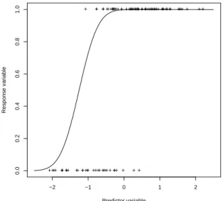
Dataset 1, presented in Figure 1, contains n = 100 observations, generated using α = 1 and
β = 2. The values of the predictor variable have been fixed at random from the standard normal
−2 −1 0 1 2 0.0 0.2 0.4 0.6 0.8 1.0 Predictor variable Response variable + + + + + + + + + + + + ++ ++ + + + + + + + + + + + + + + + + + + + + + + + + + + + + + + + + + + + + ++ + + + + ++++ ++ + + + + + + + + + + + + + + + + + + + + + + ++ + + + + + + + + + + + +
Figure 1: Dataset 1: plot of simulated data and of Φ(1 + 2q) (curve)
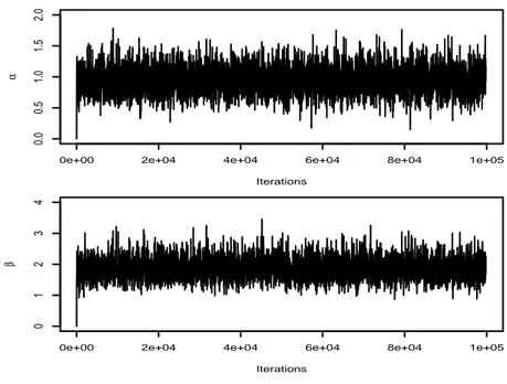
100, 000 iterations. Their behavior appear satisfactory and convergence to the stationary distribu-tion is very quick. The empirical means, based on the last 20, 000 iteradistribu-tions, are equal to 0.94 for
α and 1.85 for β. They represent MCMC estimates of the posterior expectations of α and β, and
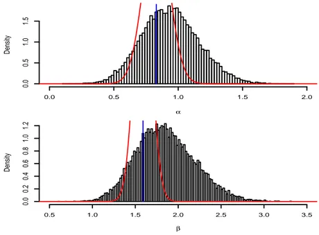
appear satisfactory. Moreover, using the empirical variances based on the last 20, 000 iterations, MCMC estimates of the posterior variance of α and β are respectively given by 0.048 and 0.12. The maximum likelihood estimates (MLEs) of α and β are equal to 0.92 and 1.79. The MLEs have been calculated using the EM algorithm: convergence was reached after 254 iterations. The optimization algorithm of the variational approximation method has converged after 179 iterations and the variational distributions of α and β are respectively N (0.83, 0.01) and N (1.59, 0.01). Fig-ure 3 shows that these approximate distributions are significantly different from the true posterior distributions estimated through their accurate Gibbs approximations. Nevertheless, for this simu-lated dataset, the expected values of α and β calcusimu-lated through the variational approximation are acceptable. However, the variance of the approximate variational posterior distribution of α and β
0e+00 2e+04 4e+04 6e+04 8e+04 1e+05 0.0 0.5 1.0 1.5 2.0 Iterations α
0e+00 2e+04 4e+04 6e+04 8e+04 1e+05
0 1 2 3 4 Iterations β
Figure 2: Dataset 1: evolution of the Gibbs Markov chains over 100, 000 iterations
are too small.
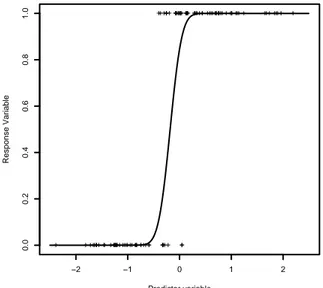
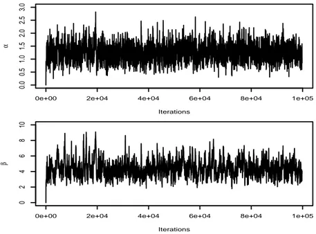
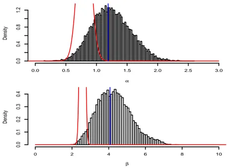
Dataset 2, presented in Figure 4, has been generated for α = 1 and β = 5. The values of the predictor variable have been fixed at random from the standard normal distribution. Figure 5 presents the behavior of the Gibbs chains over 100, 000 iterations. We observe that the convergence of these chains to their stationary distributions is as fast as in the case of dataset 1. The empirical means over the last 20, 000 iterations are equal to 1.25 for α and 4.30 for β. This is the Gibbs estimates of the posterior means of α and β. Moreover, using the empirical variances relative to the last 20, 000 iterations, MCMC estimates of the posterior variance of α and β are respectively given by 0.10 and 0.84. The maximum likelihood estimations of α and β are respectively equal to 1.19 and 4.07. These estimates have been calculated using the EM algorithm which has con-verged after 1859 iterations. The optimization algorithm of the variational approximation method has converged after 438 iterations and the variational distributions of α and β are respectively
α Density 0.0 0.5 1.0 1.5 2.0 0.0 0.5 1.0 1.5 β Density 0.5 1.0 1.5 2.0 2.5 3.0 3.5 0.0 0.2 0.4 0.6 0.8 1.0 1.2
Figure 3: Dataset 1: histograms of the last 20, 000 Gibbs simulations, variational densities (curve) and maximum likelihood estimations (straight line)
true posterior distributions estimated by their accurate Gibbs approximations. For this simulated dataset, variational approximations are very poor.
As we have just verified on a specific example, the mean-field variational approach can fail to identify the posterior location. In order to provide a further check on the performance of the method, we consider now the probit model with p = 2 and xi = (ui, vi). In this case, there two predictor variables, chosen at random from the normal distribution with mean 0 and variance 2, and no intercept. For different sample sizes with θ0= (θ
1, θ2) = (1, 2) and 100 Monte Carlo replications,
Table 1 gives a Monte Carlo approximation to the square root of the mean square difference between the Gibbs sampling approximation to the posterior mean and the mean-field variational location. For each dataset, we used 100, 000 Gibbs iterations and checked the convergence. In this case, the mean-field variational approximation to the posterior mean is reasonable even though, for small sample sizes, this approximation could be poor.
−2 −1 0 1 2 0.0 0.2 0.4 0.6 0.8 1.0 Predictor variable Response Variable + + + + + + + + ++ + + + + + + + + + + + + + + + ++ + + + ++++ + + + + + + + + + + + + ++ + + + + + + + + + + + + + + + + + + + + + + + + + + + + + + + + + + + + + + + + + + + + + + + + + ++ +
Figure 4: Dataset 2: plot of simulated data and of Φ(1 + 5q) (curve)
5
Conclusion
Variational methods have been recently popularized in order to carry out complex Bayesian infer-ences and predictions, especially in the presence of latent variables. In this note, we have described the mean-field variational method and evaluated its performance with regard to the Bayesian pro-bit model. The results we obtain are not unambiguous, and reinforce the conclusion that further investigation and testing is required before the mean-field variational method can be accepted as a reliable computational tool for Bayesian inference in a variety of applied settings.
References
Albert, J. and Chib, S. (1993). Bayesian analysis of binary and polychotomous response data. J.
American Statist. Assoc., 88:669–679.
Beal, M. (2003). Variational Algorithms for Approximate Bayesian Inference. Technical report, Gatsby Computational Neuroscience Unit. Ph.D. Thesis.
Beal, M. and Ghahramani, Z. (2002). The variational Bayesian EM algorithm for incomplete data: with application to scoring graphical model structures. In Bayesian Statistics, 7, Oxford. Oxford University Press.
0e+00 2e+04 4e+04 6e+04 8e+04 1e+05 0.0 0.5 1.0 1.5 2.0 2.5 3.0 Iterations α
0e+00 2e+04 4e+04 6e+04 8e+04 1e+05
0 2 4 6 8 10 Iterations β
Figure 5: Dataset 2: evolution of the Gibbs chains over 100, 000 iterations
Casella, G. and Robert, C. (1999). Monte Carlo Statistical Methods. Springer-Verlag.
Cowell, R., Dawid, A., Lauritzen, S., and Spiegelhalter, D. (1999). Probabilistic Networks and
Expert Systems. Springer-Verlag.
Doucet, A., de Freitas, N., and Gordon, N. (2001). Sequential Monte Carlo Methods in Practice. Springer-Verlag.
Everitt, B. (1984). An Introduction to Latent Variable Models. Chapman and Hall.
Ghahramani, Z. and Beal, M. (2001). Propagation algorithms for variational Bayesian learning. In Leen, T., Dietterich, T., and Tresp, V., editors, Advances in Neural Information Processing
Systems, 13. MIT Press.
Humphreys, K. and Titterington, D. (2000). Approximate Bayesian inference for simple mixtures. In COMPSTAT’2000, Proceedings in Computational Statistics. Springer-Verlag.
Humphreys, K. and Titterington, D. (2001). Some examples of recursive variational approximations for Bayesian inference. In Opper, M. and Saad, D., editors, Advances Mean Field Methods:
Theory and Practice. MIT Press.
Jaakkola, T. (2001). Tutorial on variational approximation methods. In Opper, M. and Saad, D., editors, Advanced Mean Field Methods: Theory and Practice. MIT Press.
Jaakkola, T. and Jordan, M. (2000). Bayesian parameter estimation via variational methods.
α Density 0.0 0.5 1.0 1.5 2.0 2.5 3.0 0.0 0.4 0.8 1.2 β Density 0 2 4 6 8 10 0.0 0.1 0.2 0.3 0.4
Figure 6: Dataset 2: histograms of the last 20, 000 Gibbs simulations, variational densities (curve) and maximum likelihood estimations (straight line)
Jordan, M. (2004). Graphical Models. Statist. Science, 19:140–155.
Jordan, M., Ghahramani, Z., Jaakkola, T., and Saul, K. (1999). An introduction to variational methods for graphical models. Machine Learning, 37(2):183–233.
Kass, R. and Raftery, A. (1995). Bayes factor and model uncertainty. J. American Statist. Assoc., 90:773–795.
Lauritzen, S. (2003). Some modern applications of graphical models. In Green, P., Hjort, N., and Richardson, S., editors, Highly Structured Stochastic Systems. Oxford University Press, Oxford. Little, R. and Rubin, D. (1987). Statistical Analysis with Missing Data. John Wiley, New York. Mclachlan, G. and Krishnan, T. (1997). The EM Algorithm and Extensions. John Wiley, New
York.
Ripley, B. (1987). Stochastic Simulation. John Wiley, New York.
Wang, B. and Titterington, D. (2004). Convergence and asymptotic normality of variational Bayesian approximations for exponential family models with missing values. In Chickering, M. and Halpern, J., editors, Proceedings of the 20th Conference in Uncertainty in Artificial
Intelligence. AUAI Press.
Wang, B. and Titterington, D. (2006). Convergence properties of a general algorithm for calculating variational Bayesian estimates for a normal mixture model. Bayesian Analysis. to appear.
θ1 θ2
n = 50 0.0881 0.1151
n = 100 0.0466 0.0588
n = 500 0.0299 0.0561
Table 1: For different sample sizes and 100 Monte Carlo replications, comparison between Gibbs sampling approximation to the posterior mean and the mean-field variational location
Wiegerinck, W. (2000). Variational approximations between mean field theory and the junction tree algorithm. In Boutilier, C. and Goldszmidt, M., editors, Proceedings of the 16th Conference