Bayesian time series models and scalable inference

Bayesian Time Series Models and Scalable Inference

by

Matthew James Johnson

B.S. Electrical Engineering and Computer Sciences, UC Berkeley, 2008 S.M. Electrical Engineering and Computer Science, MIT, 2010

Submitted to the Department of Electrical Engineering and Computer Science in partial fulfillment of the requirements for the degree of

Doctor of Philosophy in

Electrical Engineering and Computer Science at the Massachusetts Institute of Technology

June 2014

@

2014 Massachusetts Institute of Technology All Rights Reserved.

Signature redacted

MAS SACHUSETTS INST-rT E OF TECHNOLOGY

UN

_{10 2014}

LIBRARIES

Signature of Author:

Certified bv:

Department of Actrical Engineering and Computer Science May 21 2014

Signature redacted

Alan S. Willsky Edwin Sibley Webster Professor of Electrical Engineering and Computer Science Thesis Supervisor

Sianature redacted

Accepted by:

/

slie A. Kolodziejski Professor of Electrical Engineering and Computer Science Chair, Department Committee on Graduate Students

Bayesian Time Series Models and Scalable Inference

by Matthew James Johnson

B.S. Electrical Engineering and Computer Sciences, UC Berkeley, 2008

S.M. Electrical Engineering and Computer Science, MIT, 2010 Submitted to the Department of Electrical Engineering

and Computer Science on May 21 2014

in Partial Fulfillment of the Requirements for the Degree

of Doctor of Philosophy in Electrical Engineering and Computer Science

Abstract

With large and growing datasets and complex models, there is an increasing need for scalable Bayesian inference. We describe two lines of work to address this need.

In the first part, we develop new algorithms for inference in hierarchical Bayesian time series models based on the hidden Markov model (HMM), hidden semi-Markov model (HSMM), and their Bayesian nonparametric extensions. The HMM is ubiquitous in Bayesian time series models, and it and its Bayesian nonparametric extension, the hierarchical Dirichlet process hidden Markov model (HDP-HMM), have been applied in many settings. HSMMs and HDP-HSMMs extend these dynamical models to provide state-specific duration modeling, but at the cost of increased computational complexity for inference, limiting their general applicability. A challenge with all such models is scaling inference to large datasets.

We address these challenges in several ways. First, we develop classes of duration models for which HSMM message passing complexity scales only linearly in the ob-servation sequence length. Second, we apply the stochastic variational inference (SVI) framework to develop scalable inference for the HMM, HSMM, and their nonparamet-ric extensions. Third, we build on these ideas to define a new Bayesian nonparametnonparamet-ric model that can capture dynamics at multiple timescales while still allowing efficient and scalable inference.

In the second part of this thesis, we develop a theoretical framework to analyze a special case of a highly parallelizable sampling strategy we refer to as Hogwild Gibbs sampling. Thorough empirical work has shown that Hogwild Gibbs sampling works very well for inference in large latent Dirichlet allocation models (LDA), but there is little theory to understand when it may be effective in general. By studying Hogwild Gibbs applied to sampling from Gaussian distributions we develop analytical results as well as a deeper understanding of its behavior, including its convergence and correctness in some regimes.

Thesis Supervisor: Alan S. Willsky

Contents

Abstract 3

1 Introduction 9

1.1 Efficient models and algorithms for Bayesian time series analysis . . . .

9

1.2 Analyzing Hogwild Gaussian Gibbs sampling . . . . 11

1.3 Organization and summary of contributions . . . . 12

2 Background 15 2.1 G raphical m odels . . . . 15

2.1.1 Directed graphical models . . . . 15

2.1.2 Undirected graphical models . . . . 19

2.1.3 Exact Inference and Graph Structure . . . . 21.

2.2 Exponential families and conjugacy . . . .25

2.2.1 Definition and Basic Properties . . . . 25

2.2.2 C onjugacy . . . . 29

2.3 Bayesian inference algorithms in graphical models . . . . 32

2.3.1 Gibbs sampling . . . .32

2.3.2 Mean field variational inference . . . . 33

2.4 Hidden Markov Models . . . .37

2.4.1 HMM Gibbs sampling . . . .39

2.4.2 HMM Mean Field . . . . 40

2.5 The Dirichlet Process and Nonparametric Models . . . . 42

3 Hierarchical Dirichlet Process Hidden Semi-Markov Models 47 3.1 Introduction . . . 47

3.2 Background and Notation . . . .48

3.2.1 H M M s . . . . 49

3.2.2 H SM M s . . . . 49

3.2.3 The HDP-HMM and Sticky HDP-HMM . . . . 52

3.3 HSMM Models . . . . 54

3.3.1 Finite Bayesian HSMM . . . . 54

6 CONTENTS 3.3.2 HDP-HSM M ...

3.3.3 Factorial Structure ...

3.4 Inference Algorithms . . . . 3.4.1 A Gibbs Sampler for the Finite Bayesian HSMM . . . . Outline of Gibbs Sampler . . . . Blocked Conditional Sampling of (xt) with Message Passing 3.4.2 A Weak-Limit Gibbs Sampler for the HDP-HSMM . . . . . Conditional Sampling of {f7r()} with Data Augmentation . . 3.4.3 A Direct Assignment Sampler for the HDP-HSMM . . . . . Resam pling (xt) . . . .

Resampling 3 and Auxiliary Variables p . . . . 3.4.4 Exploiting Changepoint Side-Information . . . . 3.5 Experim ents . . . . 3.5.1 Synthetic D ata . . . . 3.5.2 Power Disaggregation . . . . 3.6 Sum m ary . . . . 4 Faster HSMM Inference with Efficient Representations

4.1 Introduction . . . . 4.2 Related work . . . . 4.3 HMM embeddings and HSMM messages . . . . 4.4 HSMM inference with negative binomial durations . . . . 4.4.1 An embedding for negative binomial durations . . . . 4.4.2 Gibbs sam pling . . . . 4.4.3 HMM embeddings for negative binomial mixtures . . . . 4.5 Generalizations via LTI system realization . . . . 4.5.1 LTI systems and realizations . . . . 4.5.2 LTI realizations of HSMMs . . . . 4.6 Sum m ary . . . . 55 55 57 58 58 58 59 60 64 65 67 67 68 69 71 76 79 79 80 81 87 87 90 92 93 94 95 99

5 Stochastic Variational Inference for HMMs, HSMMs, and

Nonpara-metric Extensions ₁₀₁

5.1 Stochastic variational inference . . . 102

5.1.1 _{Stochastic gradient optimization . . . 102}

5.1.2 Stochastic variational inference . . . 103

5.2 SVI for HMMs and HSMMs . . . 105

5.2.1 _{SVI update for HMMs . . . 105}

5.2.2 SVI update for HSMMs . . . 107

5.3 Linear-time updates for negative binomial HSMMs . . . 109

5.4 Extending to the HDP-HMM and HDP-HSMM . . . 113

5.5

Experim ents . . . 116 6 Scalable Inference in Models with Multiple Timescales

6 CONTENTS

CONTENTS

6.1 Introduction . . . 119

6.2 Related work . . . .20

6.3 Model specification . . . . 121

6.4 Gibbs sampling . . . 123

6.4.1 Collapsed Gibbs sampler . . . 123

6.4.2 Weak limit sampler . . . 125

6.4.3 Exploiting negative binomial durations . . . 127

6.5 Mean field and SVI . . . . 128

6.6 Experim ents . . . . 132

6.6.1 Dataset and features . . . . 133

6.6.2 Setting informative duration priors . . . . 134

6.6.3 Experimental procedure and results . . . . 136

6.7

C onclusion . . . . 139

7 Analyzing Hogwild Parallel Gaussian Gibbs Sampling 141 7.1 Introduction . . . . 1.41 7.2 R elated work . . . . 142

7.3 Gaussian sampling background . . . 143

7.4 Hogwild Gibbs model . . . 146

7.5 Gaussian analysis setup . . . 147

7.6 Convergence and correctness of means . . . 148

7.6.1 A lifting argument and sufficient condition . . . 150

7.6.2 Exact local block samples . . . ..155

7.7 V ariances . . . . 155

7.7.1 Low-order effects in A . . . 156

Block-diagonal error . . . 160

Off-block-diagonal error . . . . 162

7.7.2 Exact local block samples . . . 166

7.8 Sum m ary . . . . 167

8 Conclusions and Future Directions 169 8.1 Summary of main contributions . . . . 169

8.2 Directions of future research . . . . 71

A Hogwild Gibbs Covariance Spectral Analysis Details 175

B Numerical Evaluation of HDP-HSMM Auxiliary Variable Sampler 177

C Spectral Learning of HMM Predictive State Representations 189

Bibliography

7

CONTENTS

Chapter 1

Introduction

As datasets grow both in size and in complexity, there is an increasing need for rich, flexible models that provide interpretable structure, useful prior controls, and explicit modeling of uncertainty. The Bayesian paradigm provides a powerful framework for approaching such modeling tasks, and in recent years there has been an explosion of new hierarchical Bayesian models and applications. However, efficient and scalable inference in Bayesian models is a fundamental challenge. In the context of large datasets and increasingly rich hierarchical models, this inference challenge is of central importance to the Bayesian framework, creating a demand both for models that admriit powerful inference algorithms and for novel inference strategies.

This thesis addresses some aspects of the Bayesian inference challenge in two parts. Ill the first part, we study Bayesian models and inference algorithms for time series analysis. We develop new efficient and scalable inference algorithms for Bayesian and Bayesian nonpararnetric time series models and we discuss new model generalizations which retain both effective algorithms and interpretable structure. In the second part, we study a highly parallelizable variation on the Gibbs sampling inference algorithm. While this algorithm has limited theoretical support and does not provide accurate results or even converge in general, it has achieved considerable empirical success when applied to some Bayesian models of interest, and its easy scalability suggests that it would be of significant practical interest to develop a theoretical understanding for when such algorithms are effective. We develop a theoretical analysis of this sampling infer-ence algorithm in the case of Gaussian models and analyze some of its key properties. * 1.1 Efficient models and algorithms for Bayesian time series analysis Bayesian modeling is a natural fit for tasks in unsupervised time series analysis. In such a setting, given time series or other sequential data, one often aims to infer meaningful

states or modes which describe the dynamical behavior in the data, along with

sta-tistical patterns that can describe and distinguish those states. Hierarchical Bayesian modeling provides a powerful framework for constructing rich, flexible models based

CHAPTER 1. INTRODUCTION

on this fundamental idea. Such models have been developed for and applied to com-plex data in many domains, including speech [30, 68, 18] behavior and motion

[32,

33, 51], physiological signals [69], single-molecule biophysics [71], brain-machine interfaces

[54],

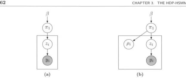
handwritten characters [67], and natural language and text [44, 70]. At their core, these models are built on a Bayesian treatment of the ubiquitous Hidden Markov Model (HMM), a model structure which provides both a coherent treatment of the notion of state and temporal dynamics as well as efficient inference algorithms based on dynamic programming and message passing.

A significant advancement for such general-purpose models was the development of the Bayesian nonparametric hierarchical Dirichlet process hidden Markov model (HDP-HMM) [106]. The HDP-HMM allows the complexity of the model to be learned flexibly from the data, and indeed allows the complexity of the representation to grow with the amount of data. However, in the case of the HDP-HMM the flexibility of the Bayesian nonparametric prior can lead to models with undesirably rapid switching dynamics, to the detriment of model interpretability and parsimony. The first work to address this issue was the development of the Sticky HDP-HMM, which introduced a global bias to encourage state persistence [31, 30]. In Johnson and Willsky [60] we generalized the Sticky HDP-HMM to the hierarchical Dirichlet process hidden semi-Markov model (HDP-HSMM), integrating work on HSMMs to allow arbitrary state-specific duration distributions in the Bayesian nonparametric setting. However, as with other HSMM models, explicit duration modeling increases the computational cost of inference, scaling quadratically with the observation sequence length while the cost of HMM inference scales only linearly. This increased computational complexity can limit the applicability of both the HDP-HSMM and the Bayesian HSMM even when non-geometric duration distributions provide a better model.

An additional challenge for all such Bayesian time series models is scaling inference to large datasets. In particular, the Gibbs sampling and mean field algorithms developed for the HMM and HSMM, as well as their nonparametric extensions, require a complete pass over the dataset in each iteration and thus do not scale well. In contrast, recent advances in scalable mean field methods require only a small number of passes over large datasets, often producing model fits in just a single pass. However, while such methods have been studied extensively for text topic models [53, 115, 17, 114, 92, 52], they have not been developed for or applied to time series models.

In this thesis we address these inference challenges in several ways. To address the challenge of expensive HSMM inference, in Chapter 4 we develop a framework for computing HSMM messages efficiently for some duration distributions. In particular, we derive message passing recursions for HSMMs with durations that are modeled as negative binomials or mixtures of negative binomials for which the computational 10

Sec. 1.2. Analyzing Hogwild Gaussian Gibbs sampling

complexity scales only linearly with the observation sequence length. We also give an HSMM Gibbs sampling algorithm which exploits this efficient structure.

To address the challenge of scaling inference to large datasets, in Chapter 5 we de-velop stochastic variational inference (SVI) algorithms for the Bayesian HMM, HSMM, and their nonparametric extensions. In addition, we build on the framework of Chap-ter 4 to develop fast approximate updates for HSMMs with negative binomial durations. We show that, as with SVI for topic models, the resulting algorithms provide speedups of several orders of magnitude for large datasets.

In Chapter 6 we build on these ideas to develop a Bayesian nonparametric time series model that can capture dynamics at multiple timescales while maintaining efficient and scalable inference. This model is applicable to settings in which the states of complex dynamical behavior can be decomposed further into substates with their own dynamics. Such behavior arises naturally in the context of speech analysis, where we may wish to model dynamics within individual phonemes as well as the dynamics across phonemes

[68,

18], and in the context of behavior analysis, where complex movements can be decomposed into component parts [51, 32]. While this model is significantly more complex than the HDP-HMM or HDP-HSMM alone, we show how to compose the ideas developed in Chapters 3, 4, and 5 to develop both efficient Gibbs sampling and scalable SVI inference.

* 1.2 Analyzing Hogwild Gaussian Gibbs sampling

Taking a broader perspective on scaling Bayesian inference, it is clear that some of the workhorse Bayesian inference algorithms cannot scale to large datasets for general models. Sampling methods in particular have proven to be hard to scale, and while there is considerable ongoing work oii scalable sampling inference [116, 42], new strategies must be developed and analyzed.

Some lines of work aim to parallelize the computation of sampling updates by ex-ploiting conditional independence and graphical model structure [42]. Though this strategy can be effective for some settings, there are many models and collapsed sam-plers in which there are no exact conditional independencies and hence no opportunities for such parallelization. However, in some cases dependence may be weak enough so that some degree of independent computation can be tolerated, at least to produce good approximate updates. In particular, thorough empirical work has shown that an extremely simple and highly parallelizable strategy can be effective, at least for one one popular hierarchical Bayesian model: by simply running Gibbs updates in parallel on multiple processors and only communicating those updates to other processors period-ically, one can effectively sample from the latent Dirichlet allocation (LDA) model [83,

82, 73, 7, 55].

CHAPTER 1. INTRODUCTION

While the empirical success in the case of LDA is well-documented, there is little theory to support this strategy. As a result, it is unclear for which other models or datasets this strategy may be effective, or how the organization of the computation, such as the frequency of synchronization and the number of parallel processors, may affect the results. However, developing a general theory may be difficult: even standard sampling algorithms for general Bayesian models are notoriously resistant to theoretical analysis, and the parallel dynamics add another layer of difficulty.

Therefore to begin to develop such a theoretical analysis we consider the case of using this parallel strategy to sample from Gaussian distributions. Gaussian distributions and algorithms are tractable for analysis because of their deep connection with linear algebra, and we exploit this connection to develop an analysis framework that provides an understanding of several key properties of the algorithm. We call this strategy Hogwild Gaussian Gibbs sampling, and in Chapter 7 we describe our analysis framework and prove several salient results concerning the convergence and correctness of Gaussian Hogwild Gibbs sampling.

U 1.3 Organization and summary of contributions

In this section we provide an outline of the rest of the thesis and a summary of our main contributions.

Chapter 2: Background

In Chapter 2 we provide a brief overview of the foundations for the work in this thesis, including probabilistic graphical models, exponential family distributions and conju-gate Bayesian analysis, hidden Markov models, and Bayesian nonparametric models constructed using the Dirichlet process.

Chapter 3: The Hierarchical Dirichlet Process Hidden semi-Markov Model We originally developed the HDP-HSMM in Johnson [59], and we include its

develop-ment here because Chapters 4, 5, and 6 build on it. There are new contributions in this chapter as well; in particular, in Chapter 3 and Appendix B we provide a thorough numerical study of the Gibbs sampler we proposed for the HDP-HSMM. The power disaggregation application is also new, in addition to the factorial HDP-HSMM model. Finally, the derivations of the Gibbs sampling algorithms are significantly improved. Chapter 4: Faster HSMM Inference with Efficient Representations

HSMM message passing is much more computationally expensive than HMM message passing, scaling as O(T2

N+TN2) compared to just O(TN 2_{) for a model with N}

states 12

Sec. 1.3. Organization and summary of contributions ₁₃

and an observation sequence of length T. This computational cost can severely limit the applicability of models based on the HSMM, especially for larger datasets.

In Chapter 4 we develop a general framework for computing HSMM messages effi-ciently for specific duration models, so that the computational complexity scales only linearly with T. The main practical result, which we use extensively in Chapters 5 and 6, is an efficient message passing recursion for HSMMs with durations that are modeled as negative binomial distributions or mixtures of negative binomial distribu-tions. We also develop a Gibbs sampling algorithm for HSMMs with negative binomial durations using these ideas.

The framework we develop is much more general, and includes new connections to the theory of linear time-invariant (LTI) systems, which could yield efficient message passing recursions for more duration models as well as new approximation schemes. Chapter 5: SVI for HMMs, HSMMs, and Nonparametric Extensions

Since scalable inference is a fundamental challenge for Bayesian time series models, in Chapter

5

we apply the stochastic variational inference (SVI) framework to develop new algorithms for Bayesian HMMs, HSMMs, and their nonparamnetric extensions, the HDP-HMM and HDP-HSMM. We show that these SVI algorithms can fit such time series models with just a single pass over large datasets.

In addition, because the computational complexity of general HSMM message pass-ing inference can be limitpass-ing even in the minibatch settpass-ing of SVI, we build on the ideas developed in Chapter 4 to develop an approximate SVI update for models with durations that are modeled as negative binomial distributions or mixtures of negative binomial distributions. We demonstrate that this approximate update can effectively fit HSMM models with time complexity that scales only linearly with the observation sequence length.

Chapter 6: Scalable Inference in Models with Multiple Timescales

In many settings we may wish to learn time series models that represent dynamics at multiple time scales, such as speech models which capture both the dynamics within individual phonemes and the dynamics across phonemes. It is crucial for such models to admit efficient and scalable inference algorithms, since such complex dynamics require larger datasets to be learned effectively.

In Chapter 6 we develop a Bayesiani nonparametric model for learning such dynamn-ics. We build on the HDP-HSMM developed in Chapter 3 so that explicit duration modeling can be used to identify dynamics at the different timescales. Using the ideas from Chapters 4 and 5 we also develop an efficient Gibbs sampler and a scalable SVI algorithm. We demonstrate the effectiveness of both the model and the proposed

infer-ence algorithms on an application to unsupervised phoneme discovery.

Chapter 7: Analyzing Hogwild Parallel Gaussian Gibbs Sampling

Scaling sampling inference algorithms to large datasets is a fundamental challenge for Bayesian inference, and new algorithms and strategies are required. One highly par-allelizable strategy, which we call Hogwild Gibbs sampling, has been shown through empirical work to be very effective for sampling from LDA models. However, there is limited theoretical analysis for Hogwild Gibbs sampling and so it is difficult to un-derstand for which models it may be helpful or how algorithm parameters may affect convergence or correctness. Furthermore, sampling algorithms for general models are notoriously difficult to analyze.

In Chapter 7 we develop a theoretical framework for Hogwild Gibbs sampling applied to Gaussian models. By leveraging the Gaussian's deep connection to linear algebra, we are able to understand several properties of the Hogwild Gibbs algorithm, and our framework provides simple linear algebraic proofs. In particular, we give sufficient conditions on the Gaussian precision matrix for the Hogwild Gibbs algorithm to be stable and have the correct process means, we provide an analysis of the accuracy of the process covariances in a low-order analysis regime when cross-processor interactions are small, and we provide a detailed understanding of convergence and accuracy of the process covariance, as well as a way to produce unbiased estimates of the exact covariance, when the number of processor-local Gibbs iterations is large.

Chapter 8: Conclusions and Recommendations

In Chapter 8 we provide concluding remarks as well as some potential avenues for future research.

Chapter 2

Background

In this chapter we provide a brief overview of the foundations on which this thesis builds, particularly probabilistic graphical models, exponential family distributions, hidden Markov models, and Bayesian nonparametric models constructed using the Dirichlet process.

* 2.1 Graphical models

In this section we overview the key definitions and results for directed and undirected probabilistic graphical models, which we use both for defining models and constructing algorithms in this thesis. For a more thorough treatment of probabilistic graphical models, see Koller and Friedman

[65].

* 2.1.1 Directed graphical models

Directed graphical models, also called Bayes nets, naturally encode generative model parameterizations, where a model is specified via a sequence of conditional distribu-tions. They are particularly useful for the hierarchical Bayesian models and algorithms developed in this thesis.

First, we give a definition of directed graphs and a notion of directed separation of nodes. Next, we connect these definitions to conditional independence structure for collections of random variables and factorization of joint densities.

Definition 2.1.1 (Directed graph). For some n E N, a directed graph on

n

nodes is

a

pair (V, E) where V = [n] {1, 2,.. .,n} and E C (V x V) \ {(ii) : V}. We call

the elements of V the (labeled) nodes or vertices and the elements of E the edges, and

we say (i, j)

E

E is an edge from i to

j.

Given a graph (V, E), for distinct i, j E V we write i -+

j

or

j

<- i if (i, j)

E

E

and write i

j

if (i,j) E E or (j, i) E E. We say there is a directed path from

11

to in of length n - 1 if for some i2, 3, . ,n- E V we have ii -+ i2 -+

i,,

and an

undirected path if we have i1-i 2 .-- in. We say node

j

is a descendant of node

i

C---

0

C-- -

C

M

(a) (b) (c)

Figure 2.1: An illustration of the cases in Definition 2.1.2. Shaded nodes are in the

set C.

if there is a directed path from i to

j,

and we say

j

is a child of i if there is a directed path of length 1. Similarly, we say i is an ancestor of

j

if

j

is a descendant of i, and we say i is a parent of

j

if

j

is a child of i. We use WG(i) to denote the set of parents

of node i and cG(i) to denote its children.

We say a directed graph is cyclic if there is a node i E V that is its own ancestor, and we say a graph is acyclic if it is not cyclic. For directed graphical models, and all of the directed graphs in this thesis, we use directed acyclic graphs (DAGs).

Using these notions we can define the main idea of directed separation.

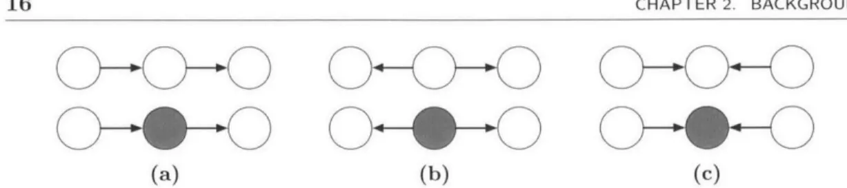
Definition 2.1.2 (Blocked/unblocked triples). Given a DAG G = (V, E), let a -b -c

be an undirected path with a, b, c E V, and let C C V be a subset of nodes with C

n

{a, c} = 0. We call a - b - c a triple, and we say it is blocked by C in two cases:

1. if the structure is not a b +- c, then b G C

2. if the structure is a -+ b <- c, and for all descendants b' E V of b we have b'

V

C.

We say a triple is unblocked by C if it is not blocked by C.

We illustrate the cases in Definition 2.1.2 in Figure 2.1, which shows six triples of nodes, where nodes in the set C are shaded. In each of (a) and (b), the top triple is unblocked while the bottom triple is blocked, corresponding to case 1 in the definition. However, in (c) the reverse is true: the top triple is blocked while the bottom triple is unblocked, corresponding to case 2 in the definition.

Definition 2.1.3 (Blocked/unblocked path). Given a DAG G = (V, E) and a set

C C V, let i1 - i2 - n be a path with C n {i1,i} = 0. We call the path

unblocked by C if every triple in the path is unblocked by C. We call the path blocked by C if it is not unblocked.

Note that Koller and Friedman [65] uses the term active trail for our definition of

unblocked path.

Definition 2.1.4 (d-separation). Given a DAG G = (V, E), for distinct i, j E V and

a subset C C V with C

n

{i, j} 0, we say i and j are d-separated in G by C

Sec. 2.1. Graphical models 17

if there is no undirected path between i and

j

that is unblocked by C, and we write

d-sepc(i,

j

C). Further, for disjoint subsets A, B, C c V with A and B nonempty we write d-sepG(A, B|C) if we have d-sepG(i, jIC) for all i C A and

j

e

B.

In words, i,

j

E V may not be d-separated in G given C if there exists an undirected path between i and

j

in G. However, the path must be unblocked, where if a node on the path belongs to C it generally blocks the path except when there is a "V" structure a -+ b +- c oi the path, in which case b blocks the path unless it or one of its

descendants is in C. This special rule is useful when defining probabilistic structure in terms of the graph because it models how independent random variables can become dependent when they are competing explanations for the same observation.

Next, we give a definition of conditional independence structure in collections of random variables that uses graphical d-separation.

Definition 2.1.5 (Markovianity on directed graphs). Given a DAG G = (V, E) and a

collection of random variables X =

{Xj

: i C V} indexed by labeled nodes in the graph, we say X is Markov on G if for disjoint subsets A, B, C C V we have

d-seP (alA, B|IC ) =-> X A -L X B|X I _2.. where for S C V we define XS

A

{Xi i E S}.

Note that this definition does not require that the graph capture all of the condi-tional independencies present in the collection of random variables. Indeed, a collection of random variables can be Markov on many distinct graphs, and every collection is Markov oi the complete graph. Graphs that capture more structure in the collection of random variables are generally more useful.

Conditional independence structure can be used in designing inference algorithms, and a graphical representation can make clear the appropriate notion of local informa-tion when designing an algorithm with local updates. A particularly useful noinforma-tion of local information is captured by the Markov blanket.

Definition 2.1.6 (Directed Markov blanket). Given a DAG G = (V, E), the Markov

blanket for node i C V, denoted MBG(i), is the set of its parents, children, and childreis' parents:

MBc(i) A

{j

E V

:j

- i}Uj E V :i -}U{j

_E

_{V : ]k} .i-± k<-j}. (2.1.2)

The Markov blanket for a set of nodes A C V contains the Markov blankets for all nodes

in A except the nodes in A itself:

MBc(A) U

U

MBG(i)

\A.

(2.1-3)

18 _{CHAPTER 2. BACKGROUND}

Figure 2.2: An illustration of the directed Markov blanket defined in Definition 2.1.6. Nodes in the Markov blanket of node i are shaded gray.

We illustrate Definition 2.1.6 in Figure 2.2. The nodes in the Markov blanket of node i are shaded gray.

Proposition 2.1.1. _{Given a collection of random variables}

_{

_{Xi : i E V} that is Markov}

with respect to a DAG G = (V, E), we have

Xi If XS XMBG(i) _(2.1.4)

where S A V

\

(MBG(i) U {i}).

Proof. By conditioning on the parents of node i, all paths of the form a -+ b -* i are

blocked. By conditioning on its children, all paths of the form i -> b - c are blocked.

By conditioning on the childrens' parents, all paths of the form i - b <- c, which may have been unblocked by conditioning on b or one of its descendants via case 2 of

Definition 2.1.4, are blocked. _D

Another common and convenient notion of probabilistic graphical structure is a density's factorization with respect to a DAG.

Definition 2.1.7 (Factoring on directed graphs). Given a DAG G = (V, E) on n nodes

and a collection of random variables X =

{Xi

: i C V} with density px with respect to

some base measure, we say px factorizes according to G if we can write

PX(Xi, . ., z) = rl P(XiIz, e(j)) (2.1.5)

iEV

Sec. 2.1. Graphical models

Theorem 2.1.1. A collection of random variables {Xi : I

E

V} with a joint density

(with respect to some base measure) is Markov on a DAG G if and only if the joint density factorizes as in Eq. (2.1.5).

Proof. The proof is straightforward. In Koller and Friedman [65], Theorem 3.1 shows

Markovianity implies the densities factor and Theorem 3.2 shows the reverse. D * 2.1.2 Undirected graphical models

Undirected graphical models, also called Markov random fields, do not easily encode generative model specifications. However, they

can

be more useful for encoding soft con-straints or local partial correlations. We use an undirected graphical model perspective in our analysis of Hogwild Gibbs Sampling in Chapter 7.

As with directed graphical models, we first define undirected graphs and a notion of separation of nodes, then give definitions that link the graphical structure to both conditional independence structure in a collection of random variables and factorization structure in the joint density for those variables.

Definition 2.1.8 (Undirected graph). For some n E N, an undirected graph on n

nodes is a pair (V, E) where V =

[n]

and E C {{i,

j}

: i, j E V, i / J}.

Analogous to the definition in the previous section, there is a natural notion of an undirected path between nodes. Given a graph (V, E), for distinct i,

j

E V we write

i

j

if {i, E} F, and we say there is an (undirected) path from i₁ to i, of length ri - 1 if for some i2, i6, - , in- 1 E V we have 11- i2 - -n. We say i is a neighbor of

j

if {ij} E E and denote the set of neighbors of node i as nG(i)

A

{j

E V : {i,j} c E}.

We say a pair of nodes is connected if there exists an (undirected) path from i to

_j.

The notion of undirected separation and corresponding notion of Markovianity on undirected graphs is simpler than those for directed graphs.

Definition 2.1.9 (Undirected separation). Given an undirected graph G = (V, E), for

distinct i,

j

e

V and a subset C c V with C n {i, J} = 0, we say i and

j

are separated

in G given C and write sepG(i, j|C) if there is no path from i to

j

that avoids C. For

disjoint subsets A, B, C

c

V with A and B nonempty we write sepG(A, BIC) if we have

sepG(i, jIC) for all i c A and j G B.

Definition 2.1.10 (Markovianity on undirected graphs). Given an undirected graph

G = (V, E) and a collection of random variables X = { Xi : i E V} indexed by labeled

nodes in the graph, we say X is Markov on G if for disjoint subsets A, B, C C V we have

sepG(A, B|C) -> XA L XBXC. (216

19

As with Markovianity with respect to directed graphs, an undirected graph may not encode all the conditional independence statements possible for a given collection of random variables.

The notion of Markov blanket for an undirected graph is also simpler.

Definition 2.1.11 (Undirected Markov blanket). Given an undirected graph G

(V,

E), the Markov blanket for each node i C V, denoted MBG(i), is the set of neighbors of node i:

MBG(i) nG(i)

{j

E 17: {i,j} G E}. (2.1.7)

The Markov blanket for a set of nodes A C V is the set of all neighbors to nodes in A excluding those in A:

MBG(A) U

U

MBG(i) A. (2.1.8)

icA

We can use this definition for an undirected analog of Proposition 2.1.1.

Proposition 2.1.2. Given a collection of random variables

{

Xi : i G V} that is Markov with respect to an undirected graph G = (V, E), we have

Xi LL XsIXMBG(i) (2.1.9)

where S A V \ (MBG(i) U {i})

Proof. Because all the neighbors of i are in MBG(i), for any

j

c S there can be no

undirected path from j to i that avoids MBG(i). El

We can also define a density factorization with respect to an undirected graph, though we must first define the notion of a clique. A clique in a graph (V, E) is a nonempty subset of fully-connected nodes; that is, a nonempty set C C V is a clique if for every distinct i, j C C we have {i,j} C E.

Definition 2.1.12 (Factoring on undirected graphs). Given an undirected graph G

(V,

E) and a collection of random variables X =

{X

: i C V} with density px with

respect to some base measure, we say px factorizes according to G if we can write

PX (X1, . ,n) = Z 11 Oc (xC) (2.1.10)

CEC

for a collection of cliques C of G and nonnegative potentials or factors

{4'c

: C C C} indexed by those cliques, where

Z fj0C(c)v(d)(

'CEC

Sec. 2.1. Graphical models

is a normalizing constant.

Note that cliques typically overlap; that is, we may have

Ci

n

Cj

7 0 for distinct C, C

E

C. To remove many possible redundancies, without loss of generality one can

assume that C includes only maximal cliques, where a maximal clique cannot have any other node added to it and remain a (fully-connected) clique.

The correspondence between a collection of random variables being Markov on an undirected graph and its joint density factorizing as Eq. (2.1.10) is not quite as simple as that for directed graphs because deterministic relationships among the random variables call prevent factoring the density, as shown in the next example.

Example 2.1.1. Using Example

4.4 from

Koller and Friedman [65j, consider four

binary random variables X = {Xi : i = 1, 2, 3, 4} with a PMF that takes value 1/8 on the configurations of (Xi, X2, X3, X4) given by

(0,0,0,0) (1,0,0,0) (1,1,0,0) (1,1,1,0) (0,0,0,1) (0,0, 1,1) (0, 1,1,1) (1,1,1, 1)

and 0 elsewhere. Then X is Markov on the graph 1 - 2 - 3 ---4 -- 1 but the density

cannot be factorized into pairwise potentials.

This issue cannot arise when we restrict our attention to strictly positive densities.

Theorem 2.1.2. Given a collection of random variables X = {Xj i G V} with a joint

density px (with respect to some base measure) and an undirected graph G, we have

1. If px factorizes according to G, then X is Markov on G.

2. If X is Markov on G and px is strictly positive, then Px factors according to G.

Proof. The proof for 1 is straightforward and is given as the proof of Theorem 4.1 in

Koller and Friedman [65]. The proof for 2 is the proof of the Hammersley-Clifford theorem, given as Theorem 4.8 in Koller and Friedman [65].

U 2.1.3 Exact Inference and Graph Structure

Given some specification of a probability distribution, inference for that distribution means computing quantities of interest such as marginals, conditionals, or expectations. In the graphical model framework we cal be precise about the computations required to perform inference and their complexity, as we overview in this subsection. For concreteness, we focus on undirected models with densities.

Consider an undirected graphical model specified by an undirected graph G = (V, E) and a set of potentials {ic : C E C} on a set C of cliques of G. The joint density is

proportional to the product of the clique potentials p(x)

o

Hcec

4cxc).

We can represent an arbitrary inference query in terms of a subset of nodes on which we con-dition, a subset of nodes which we marginalize out, and a subset over which we want to represent the resulting density; that is, we partition the set of nodes V into three disjoint (possibly empty) subsets A1, A2, A3 with A1 U A2 U A3 = V and write

p(xA₁| XA3) JP(XA1, xA2 JXA3 )iv(dXA 2) =

fH~

bc(xc)v(dXA2) (2.1.12)

f

H

c

0 c

(xc)v(dxA

_{1 uA}2)

Therefore to compute an arbitrary inference query we need only to compute integrals of products of the factors in the density. To simplify notation, we write such computations in the form

fJ

1

C(xC)v(dxA) (2.1.13)

CeC

for some subset A C V.

Graph structure affects how we can organize a computation of the form (2.1. 13) and thus its computational complexity. Consider the special case of integrating out a single variable xj by partitioning the set of cliques into those which contain node

j

and those which do not, Cj {C E C: j E C} and Cj {C E C: jd C}, and writing

J1

H

c(xc)v(dxj) =

J

0c\.(xc\ 3)J

fJ

V)cj(xc)v(dxj) (2.1.14)

CEC Cy ECy Ci eC₃

= 1 O Cu (xce )OB(xB) (2.1.15)

C\j EC\j

where B A {i c _{Cj : Cj E Cy}\{j} is the set of all indices that share a clique with node}

j

in G and OB is a new factor on the clique B resulting from the integral over xj. Thus as a result of the integral there is an induced graph on V

\

{j}

formed by eliminating

j

by fully connecting its neighbors and deleting it from the graph.

When integrating over multiple variables, the process repeats: given an elimination

order, nodes are eliminated one by one from the graph, and each elimination introduces

a new clique in the graph and a corresponding new potential term in the density over the remaining variables. The computational complexity of the process is determined by the size of the largest clique encountered. In the case of PMFs with finite support, the number of entries in the table encoding the new potential formed in (2.1.15) is typically exponential in the size of the new clique; in the case of PDFs, the complexity depends on the complexity of integrating over factors on cliques, where the clique size determines the number of dimensions in the domain of the integrand, and the complexity

Sec. 2.1. Graphical models

of representing the result. The optimal elimination order is itself NP hard to find for general graphs.

Some classes of graphs have straightforward elimination orderings that avoid the growth in clique size, and inference in distributions that are Markov on such graphs avoids the corresponding growth in complexity.

Definition 2.1.13 (Tree graph). A directed or undirected graph G = (V, E) is a tree

if for each pair distinct nodes i,

j

C

V there is a unique undirected path from i to

j

in

G.

In an undirected tree G, we refer to the nodes i with only single neighbors

InG

( 1 as leaves. In a directed tree, we refer to the nodes with no children as leaves.

Proposition 2.1.3 (Markov on trees). A density p that factors on an undirected tree

(V, E) can be written in terms of pairwise factors {<i: {i,

j}

C E} as

1

p(r) W= H Oiji, X). (7 (2.1.16)

{i,j}GbE

Proof. All of the maximal cliques in an undirected tree are of size at most 2. E

Note that because the edges are undirected, Oij and Oji denote the same object. Given a density that factors according to an undirected tree specified in terms of its pairwise factors {ij :

{i,

j}

E} we can convert it to a directed specification by local

normalization, i.e. by choosing a direction for each edge and computing

pXzilzg) = . Oi j .X (2.1.17)

J, Oij(Xi,Xj) v (dxj,)

Note that a density that factors on a directed tree may not in general be written purely in terms of conditional probability factors that depend only on pairs of nodes, as shown in the next example.

Example 2.1.2. A density that factors according to the directed tree G = (V, E) with

V = {1, 2, 3} and edges 1 -+ 2 <- 3 may include a factor p(x2I1, X:3). Such a density is not Markov on the undirected tree G' = (V', E') with V' = V and edges 1 - 2 -3, and instead only factors on the complete undirected graph with edges 1 - 2 - 3 -1.

Directed trees in which each node has at most one parent avoid this issue, and we can convert freely between directed and undirected tree parameterizations for such models.

Proposition 2.1.4. A density p that factors on a directed tree G = (V, E) in which each node only has one parent, i.e.

|rrG(i)

< 1 for i e V, also factors with respect to

the undirected tree G' = (V', E') formed by dropping the directions on the edges of G, i.e. V' = V and E' = {{i, j} : (i, j) E}

Proof. Set Oij (xi, xj) = p(xi I j).

With undirected trees and directed trees in which each node has at most one parent we can perform elimination without introducing larger factors by using an elimination order that recursively eliminates leaves. Furthermore, the corresponding partial sums for all such elimination orderings can be computed simultaneously with an efficient dynamic programming algorithm, as shown in the next theorem.

For an undirected graph G =

(V,

E) and a subset of nodes A C V, we define G

\

A

to be the graph formed by deleting the nodes A and the edges incident on nodes in A, i.e. the graph (V', E') where V'= V\A and E' = {{i,j} e E: i,

j

V A}. We say a pair

of nodes is connected if there exists an undirected path from i to

j,

and we say subsets

A, B

c

V are connected if there exists an i

E

A and

j

E

B that are connected.

Definition 2.1.14 (Tree messages). Given a density with respect to a base measure v that factorizes on an undirected tree G = (V, E) of the form (2.1.16), we define the

message from node i to node

j

with

{i,j}

E

E to be

mJ-4i(xi) A j 11 Vg/y (Xil, Xj)@ij (Xi, Xj) v(dxv') (2.1.18)

where (V', E') is the subtree of G that is disconnected from node i in G

j}.

Theorem 2.1.3 (Tree message passing). For a density that factorizes on an undirected

tree G = (V, E) of the form (2.1.16), the result of any computation of the form (2.1.13) can be written in terms of messages as

j 11

0(xj, xj)v(dXA)

y = ri oij (Xi, Xj) rl mnj- (Xk) (2.1.19)

{ij}E {i,j}E' kEB

where (V', E') = G\ A is the graph over the the nodes that are not integrated out and B is the set of nodes in V' that have edges to A in G, i.e. B {k C 1': {k, j} E, j

e

A}. Furthermore, all messages can be computed efficiently and simultaneously via the

recursions

mnisj (xj) = Oij (Xi, Xj ) Tnm--+k(xj)v(dxj). (2.1.20)

k EnG (j)\{i}

Therefore all inference queries in undirected trees can be computed in time linear in the length of the longest path in the tree.

Proof. The theorem follows from applying elimination to trees and expressing every

partial elimination result as (2.1.20). E

Sec. 2.2. Exponential families and conjugacy 25

We refer to an implementation of the recursion (2.1.20) as a tree message-passing

algorithm. We use tree message passing algorithms extensively as subroutines in the

inference algorithms for the time series models that we develop in the sequel.

* 2.2 Exponential families and conjugacy

In this section, we define exponential families and give some of the properties that we use in this thesis.

* 2.2.1 Definition and Basic Properties

Definition 2.2.1 (Exponential family). We say a family of densities p with respect to

a base measure v indexed by a parameter vector 0 is an exponential family of densities if it can be written as

p(xj0) = h(x) exp{'r/(0), t(x)) - Z(r;(0))} (2.2.1)

where

(-,-)

is an inner product on real vector spaces. We call tl(0) the natural parameter

vector, t(x) the (sufficient) statistic vector, h(x) the base density, and

Z (rF) Ill e, c IM

~

h (x)v1,(dx) (2.2.2)

the log partition function.

It is often useful to parameterize the family directly in terms of q, in which case we simply write the density as p(xjrj). Note that marginalizing over part of the support of ami exponential family, such as marginalizing over one coordinate of x or of t(x), does not in general yield another exponential family.

Given an exponential family of the form (2.2.1) we define the set of natural paramn-eters that yield valid normalizable probability densities as 0, where

a

ffl : Z(r/) < 00} (2.2.3)

and the set of realizable expected statistics as

M

{Ex-p(r)Lt(X)1

:

r

0 (2.2.4)

where X ~ p( - 17) denotes that X is distributed with density p( - ?j). We say a family is regular if 0 is open, and minimal if there is no nonzero a such that

(a,

t(x)) is equal

to a constant (v-a.e.). Minimality ensures that there is a unique natural parameter for each possible density (up to values on sets of v-measure 0). We say a family is tractable

CHAPTER 2. BACKGROUND

if for any r, we can evaluate Z(r) efficiently' and when X - p( . ij) we can compute E[t(X)] and simulate samples of X efficiently.

For a regular exponential family, derivatives of Z are related to expected statistics. Proposition 2.2.1 (Mean mapping and cumulants). For a regular exponential family

of densities of the form (2.2.1) with X ~ p( - I), we have VZ :

e

-+ M and

VZ(TI) = E[t(X)] (2.2.5)

and writing p

A

E[t(X)] we have

V2Z(1) = E[t(X)t(X) T] - pT. (2.2.6)

More generally, the moment generating function can be written

Mx(s) = E[e(s'X)] = ez(7s)-Z(). (2.2.7)

and so derivatives of Z generate cumulants of X, where the first cumulant is the mean and the second and third cumulants are the second and third central moments, respec-tively.

Proof. Note that we require the family to be regular even to define VZ. To show 2.2.5,

using v as the base measure for the density we write

V -Z(g) Vj ln e(qt(x) h(x)v(dx) (2.2.8)

I t (X)eC 7t(x)h h(x)v1(dx) _(2.2.9)

f Ce(rl' ))h (x) v(dx)

J t(x)p(x r)v(dx) (2.2.10)

E[t(X)]. (2.2.11)

To derive the form of the moment generating function, we write

E[e(s'X)] - fesx)p(x)v(dx) (2.2.12)

-=f e()e(7,t())-Z()h(x)v(dx) (2.2.13)

- ez(+s)-z(n). (2.2.14)

'We do not provide a precise definition of computational efficiency here. Common definitions often correspond to the complexity classes P or BPP [3].

Sec. 2.2. Exponential families and conjugacy

The cumulant generating function for X is then in Mx (s) = Z(

+

s) - Z(7D). E When a specific set of expected statistics can only arise from one member of an exponential family, we say the family is identifiable and we can use the moments as an alternative way to parameterize the family.

Theorem 2.2.1 (Exponential family identifiability). For a regular, minimal

exponen-tial family of the form (2.2.1), V Z : 0 -+ M is injective, and VZ : - M is

surjective, where M denotes the interior of A. Therefore VZ : 0 -+ A' is a bijec-tion.

Proof. See Wainwright and Jordan [113, Theorem 3.3]. D

When parameterizing a regular, minimal exponential family in terms of expected statistics [t E

M

', we say it is written with mean parameters, and we have

rI(p)=

(VZ)-1(p) using Theorem 2.2.1. Given a set of moments, the corresponding minimal exponential family member has a natural interpretation as the density (relative to v) with maximum entropy subject to those moment constraints

[113,

Section 3.1].

For members of an exponential family, many quantities can be expressed generically in terms of the natural parameter, expected statistics under that parameter, and the log partition function.

Proposition 2.2.2 (Entropy, score, and Fisher information). For a regular exponential family of densities of the form (2.2.1) parameterized in terms of its natural parameter

r/, with X ~ p( - |rj) and p(/) ) E[t(X)] we have

1. The (differential) entropy is

H[p] A -E[lnp(Xlr)] = -(r, p(r)) + Z(r). (2.2.15)

2. When the family is regular, the score with respect to the natural parameter is 'v(x, i1) Vr, lr p(Xr1) = t(x) - p(q) (2.2.16)

3. When the family is regular, the Fisher information with respect to the natural

pararmeter is

I(r) E E[v(X, 'r)v(X, ir) T 2Z](2.2.17)

Proof. Each follows from (2.2.1), where 2.2.16 and 2.2.17 use Proposition 2.2.1. D When the family is parameterized in terms of some other parameter 0 so that

r

= r(0), the properties in Proposition 2.2.2 include Jacobian terms of the form Dr//0.

CHAPTER 2. BACKGROUND

When the alternative parameter is the mean parameter p, since 1(p) = (VZ)-'(p) the relevant Jacobian is (V2Z)-1. We use the Fisher information expression (2.2.17) in the development of a stochastic variational inference (SVI) algorithm in Chapter 5.

We conclude this subsection with two examples of exponential families of densities. Example 2.2.1 (Gaussian). The Gaussian PDF can be parameterized in terms of its

mean and covariance (p, E), where 1t E Rd and E

E

Rdxd with E >- 0, and can be

written

p(xIp, E) = (27)-d/2 I -1/2 exp (X _ ,j)TE-1( _ P

= 2r-d/2 E-1 E-1 _, TE-1 T

=(21r7)/ exp{(Zl H 111 -t p), (miT I, X1) In I EnZ

hN(X) N(A, _{NN(X) ZN (7N}

where ((A,b,c), (D,e, f)) = tr(AT D)+bT e

+

cf. Therefore it is an exponential family of

densities, and further it is a regular exponential family since 0 = {( E, 1t) : E 0, p C

Rd} is open (in the standard product topology for Euclidean spaces). The family is minimal because there is no nonzero (A, b, c) such that ((A, b, c), tN(x)) = xTA b TX+c

equal to a constant (v-a.e.).

Example 2.2.2 (Categorical). Consider drawing a sample X from a finite distribution

with support on [K] = {1, 2, ... , K}, where p(x = k|7) = ,rk for K G [K] and 7r satisfies

Ei

7i = 1 and w > 0 element-wise. We can write the PMF for X as

K K

p(xIr) =

7

r

w

= exp

{

ln 7rkL[x = k]} exp

{(ln

7, 1)} (2.2.18)

k=1 k=1

where the log is taken element-wise,

I[

]

is an indicator function that takes value 1 when its argument is true and 0 otherwise, and 1

k is an indicator vector with its ith entry

E[k = i]. We call this family of densities the categorical family, and it is an exponential

family of densities with natural parameter qj(7) = In r and statistic t(x) = 12. (A

closely related family is the multinomial family, where we consider drawing a set of n independent samples from the same process, x =

{xi

: I

E

[n]}, and defining the statistic to be the counts of each occurrence, i.e. the kth entry of t(x) is

|{x,

: xi = k}|.)

Note that Z(QT) = 0. The categorical family as written in (2.2.18) is not a regular exponential family because 0 = {w7

e

RK : 71i = 1, 7 > 0} is not open. Since

the family is not regular, (2.2.16) does not apply. We can instead write the family of densities as

p(x 1r) = exp

{(ln

r, 1) - In E r} (2.2.19)

where Z(T7(it)) = In E 1 ri so that 0 {iTr

R

K : 7F > 0} is open. However, neither 28