Improved Bayesian network configurations for random variable identification of concrete chlorination models

(1)

HAL Id: hal-01270458

https://hal.archives-ouvertes.fr/hal-01270458

Submitted on 7 Feb 2016

HAL is a multi-disciplinary open access archive for the deposit and dissemination of sci-entific research documents, whether they are pub-lished or not. The documents may come from teaching and research institutions in France or abroad, or from public or private research centers.

L’archive ouverte pluridisciplinaire HAL, est destinée au dépôt et à la diffusion de documents scientifiques de niveau recherche, publiés ou non, émanant des établissements d’enseignement et de recherche français ou étrangers, des laboratoires publics ou privés.

Improved Bayesian network configurations for random

variable identification of concrete chlorination models

Thanh-Binh Tran, Emilio Bastidas-Arteaga, Franck Schoefs

To cite this version:

Thanh-Binh Tran, Emilio Bastidas-Arteaga, Franck Schoefs. Improved Bayesian network configura-tions for random variable identification of concrete chlorination models. Materials and Structures, Springer Verlag, 2016, In press, �10.1617/s11527-016-0818-4�. �hal-01270458�

(2)

Please cite this paper as:

Tran T-B, Bastidas-Arteaga E, Schoefs F (2016). Improvement of Bayesian network configurations for random variables identification in deterioration modelling. Materials and Structures. In press http://doi.org/10.1617/s11527-016-0818-4

Improved Bayesian network configurations for random variable identification of concrete chlorination models

Thanh-Binh Tran1, Emilio Bastidas-Arteaga1*, Franck Schoefs1

1_{LUNAM Université, Université de Nantes-Ecole Centrale Nantes, GeM, Institute for Research in Civil and}

Mechanical Engineering/Sea and Littoral Research Institute, CNRS UMR 6138/FR 3473, Nantes, France Abstract: Relevant material and environmental parameters are required in modelling chloride ingress into concrete. They could be determined from experimental data (concrete cores taken during inspection) but in practice data availability is limited by time-consuming and expensive tests. Consequently, the main objective of this paper is to develop an approach based on Bayesian networks (BN) to improve the parameter identification when inspection data is limited. We aim at proposing appropriate inspection configurations that reduce inspection costs and identification errors for different exposure conditions and materials. It was found that it is possible to define an optimal number of inspection points in depth for allowed identification errors defined by decision makers. The optimal number of inspection points depends on both exposure and material properties. The random variables identified with the improved BN configurations are used to assess the probability of corrosion initiation. The results indicate that the improved BN configurations are useful to identify model parameters even from scarce inspection data.

Keywords: Chloride ingress; corrosion; reinforced concrete; uncertainties; Bayesian network; identification; Inspection; Deterioration modelling.

1. Introduction

Reinforced concrete (RC) structures located close to the seashore or in contact with de-icing salts are subjected to chloride-induced corrosion deterioration. Corrosion of rebars affects load carrying capacity through various mechanisms: reduction of reinforcement cross-section, loss of bond between steel and concrete, concrete cracking and delamination [1–3]. These mechanisms reduce their serviceability and safety levels during the whole service life. Thus, the assessment of the chloride content in concrete is an important task to determine corrosion initiation risks and therefore to plan and quantify maintenance operations of structures [4–7].

Various condition assessment techniques consisting of destructive and non-destructive methods have been developed to assess chloride ingress. Destructive inspection techniques (coring), could provide accurate inspection results, however, they are more expensive and time-consuming. Non-destructive techniques are less expensive but require still technical developments [8–10] and specific post-treatment methods for assessing the chloride content from multi-technique measurements [9–12]. Data collected after inspection campaigns are often used to determine parameters for chloride ingress or corrosion propagation models. This information is helpful for lifetime

*_{Corresponding author. Address: 2 rue de la Houssinière BP 99208, 44322 Nantes Cedex 3 France.}

(3)

2

assessment and optimisation of maintenance strategies. This study focuses on the corrosion initiation stage that is estimated from chloride penetration models. Under natural exposure conditions, chloride ingress involves important uncertainties related mainly to material properties and exposure conditions [1, 6, 13–17]. These uncertainties are also affected by temporal and spatial variability of associated deterioration processes and their characterisation requires larger amount of inspection data [18–22]. Nevertheless, in real practice, the number of inspections is limited by the difficulties to implement tests that increase inspection times and costs. Therefore, it is necessary to use the available information in the best way for uncertainty quantification by using statistic and/or probabilistic methods. An appropriate method to deal with this kind of issue is to use metamodels. To characterize the randomness of model parameters, the metamodels should also introduce a function for random parameter identification. Metamodels can be categorised into two groups: response surface methods and networks. The group of response surface methods (physical response surface, polynomial response surface, polynomial Chaos expansion, etc) cannot ensure a good convergence for the results and for solving the inverse stochastic problem, they also require a very large number of coefficients [23]. In contrast, metamodels methods based on networks (Neural network, Bayesian network (BN)) can bring a fast convergence independently of the choice of the initial condition. Among this group, Bayesian network (BN) is an robust method with some characteristics which meet the demand of chloride ingress model’s data, for example: (i) BN can readily handle incomplete data set, (ii) BN can allow to learn about causal relationships, (iii) BN can deal with discrete evidences, and (iv) BN in conjunction with Bayesian statistical techniques facilitate the combination of domain knowledge data. Consequently, BN are considered in this study to deal with this problem.

Bayesian networks were used in previously for parameter identification purposes. Some studies [24–27] proposed an approach based on the use of BN updating from experimental data. They showed, after identification, a good agreement between numerical predictions and experimental measurements. In this study, we search for improved BN configurations that reduce the amount of inspection data for parameter identification. Based on the approach proposed by Tran et al. [27], data from numerical simulations, representing inspection data is used to identify information about two chloride ingress model parameters: chloride surface concentration (Cs) and the chloride

diffusion coefficient (D). Various cases representing different exposure conditions and material quality are investigated. Optimal configurations for each analysed case are suggested by evaluating the identification errors.

A brief description of the BN and its application for chloride ingress modelling are presented in section 2. Section 3 presents the procedure for the improvement of the BN configuration for parameter identification. Section 3 describes the different studied cases and the approach to select an optimal configuration of BN for each case. Finally, the identified parameters are employed in Monte Carlo simulation for the assessment of the probability of corrosion initiation (section 4).

(4)

3

2. Chloride ingress modelling and identification by using Bayesian networks

2.1. Bayesian networks theory

Generally, a BN is Direct Acyclic Graph (DAG) consisting of a set of nodes that are connected by edges to illustrate their dependencies. Nodes in BNs are graphical representation of objects and events that exist in the real world and can be presented as continuous or discrete random variables. To each child node with its parents is assigned a conditional Probability Density Function (PDF), f(X|pa(X)) or Probability Mass Function (PMF), p(x|pa(X)), where pa(X) represents for parents of X in the graph. An edge may represent causal relationships between the variables (nodes) but this is not a requirement. The graphical structure of a BN reflects the conditional independence assumption among the random variables. Hence, a BN is a compact model representing the joint PDF or PMF among random variables. In this study, only BNs with discrete random variables are considered. Figure 1 illustrates a simple BN that consists of three nodes representing to three discrete random variables X1, X2 and X3 in which X2 and X3

(2)

(3)

The summation operations in the second line of Eq. (3) are performed in a smaller domain and imply node eliminations. The calculation order starts from the last term on the right to the left, hence X3 is the first node to eliminate followed by node X2.

Elimination order is arbitrary and the size of the domains to handle due to elimination order defines the complexity of inference. Therefore, the objective of exact inference algorithms is to determine the elimination order yielding the smallest domains to handle [28]. Among exact inference algorithms, junction tree inference which can be seen as an

(5)

4

extension of node elimination, can compute the a posteriori probabilities for all nodes in a BN simultaneously and consider multiple evidences cases. The junction tree algorithm is selected for inference of all BNs in this paper.

2.2. Application to chloride ingress

2.2.1. Chloride ingress and modelling

In saturated concrete, the Fick’s diffusion equation [29] is usually used to assess unidirectional chloride ingress at a distance x from the concrete surface:

2 2 c c f f C C D t x ∂ ∂ = ∂ ∂ (4)

where Cfc (kg/m3) is the concentration of chloride dissolved in pore solution, t (year) is

the time and D (m/s2_{) is the effective chloride diffusion coefficient. Assuming that, at a} given scale, concrete is a homogeneous and isotropic material with the following initial conditions: (i) the concentration is zero at time t = 0 and (ii) the chloride surface concentration is constant during the exposure time, the free chloride ion concentration

C(x,t) at depth x after time t for a semi-infinite medium is:

C x,t

( )

= C_s 1−erf x 2 D⋅t ⎛ ⎝ ⎜⎜ ⎜⎜ ⎞ ⎠ ⎟⎟⎟ ⎟ ⎡ ⎣ ⎢ ⎢ ⎤ ⎦ ⎥ ⎥ (5)

where Cs (kg/m3) is the chloride surface concentration and erf(.) is the error function.

Eq. (5) remains valid when RC structures are saturated and subjected to constant concentration of chlorides on the exposure surfaces. In real structures, these conditions are rarely presented because concrete is a heterogeneous material and the chloride concentration in the exposed surfaces could be time-variant. Besides, this solution does not consider chloride binding capacity, concrete aging and other environmental factors such as the influence of surrounding temperature and humidity in chloride ingress process [13, 16, 30–32]. Although this solution neglects some important physical phenomena, this model is used herein to illustrate the proposed methodology for the identification of random variables using BN because its complexity is sufficient to account for non-linear effects in x-direction and in time and to perform sensitivity analyses. The methodology can be after extended to more realistic chloride ingress models: only the computation time for building the model will increase from the larger number of variables involved and consequently the larger size of the BN on one hand and the computation time of the model itself on the other one.

2.2.2. Bayesian network identification of chloride ingress model parameters

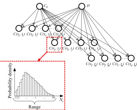
Chloride ingress could be modelled by the BN described in Figure 2 where Cs and D are

the two parent nodes representing the random variables to identify. There are n child nodes C(xi, tj) representing the discrete chloride concentration measurement in time and

space – i.e. at depth xi and at inspection time tj. Adding/removing nodes therefore

account for the discretisation in space (number of points of measurements) and time (number of inspections times). The total number of child nodes n which represents the number inspection points is computed as:

x t

n n n

=

(6)

where nx is the total number of points in depth and nt is the total number of inspection

(6)

5

C(xi, tj) could be easily estimated from Eq. (5). Both exact and approximate inference

algorithms can be used to update probabilities of the BN described in Figure 2. Exact inference is useful to analytically compute the conditional probability distribution over the variables of interest. However, they can only be applied to a very limited set of cases: when all nodes are discrete or when all nodes have linear Gaussian distribution. In the case of complex and densely connected BNs, exact inference may require intractably amount of computational time and approximate inference can be seen as an alternative. Most of approximate algorithms are based on stochastic sampling. However, these techniques still have some algorithmic difficulties that provide some limitations in the rate of convergence [33, 34]. In this study, chloride ingress model is described in an analytical form and the number of parent nodes (parameters to identify) is limited. Exact inference algorithms could therefore be difficult to apply here regarding their shortcomings. Continuous parameters are then replaced by discrete random variables. However the discretisation of continuous random variables generates approximation errors depending on the discretisation of the problem. Each node is defined over a specific range (upper and lower bounds) and discretised into a given number of states per node, Ns. The range should in theory contain all the possible values of each

parameter. These ranges can be defined on the basis of existing databases, similar study cases, or expert knowledge. Here, the ranges for Cs and D were defined enough large to

contain values representative of the variability of environmental exposure and material properties when the prior information about these parameters is very poor. The theoretical distributions presented in Table 1 can be used in this case to estimate upper and lower bounds for a given confidence interval. The adopted values cover a confidence interval larger than 99% by ensuring that the parameters to identify belong to this wide a priori range. Figure 2 also illustrates the discretisation considered for each node. For example, the node C(x1,tj) was divided into Ns = 50 states over a predefined

range. In this BN, if all nodes are discrete, the probability of chloride concentration

p(C(xi, tj)) can be calculated as follows [24, 35]:

p C x

(

( )

_i,t_j

)

= p C x

(

( )

_i,t_j | D,C_s

)

D,C_s

∑

p D,C

(

_s

)

(7) With assumption that Cs and D are two independent variables, the joint probability

of Cs and D can be rewritten as p(D, Cs) = p(D) p(Cs).

The BN allows entering evidences and then updating the probabilities in the network. In this study, the evidences could be computed from measures of chloride concentration at given points and times (chloride profiles). Let us denote Cxt1, Cxt2,…, Cxtn as n measurements obtained at depth xi and inspection time tj:

C 1≤i≤n_x 1≤ j≤nt x_i,t_j

( )

the Conditional Probability Tables (CPT). Monte Carlo simulations of the model (from Eq. (5)) are used for the computation of CPT [27]. Supposing that k observations: Cxt1, Cxt2,…,Cxtk can be used to update the BN, we aim at computing the a posteriori

distributions p(Cs|o) and p(D|o) as:

)

= p C

(

_s, D | o

)

Cs

∑

(9)

(7)

6 where:

(10) These a posteriori distributions can be estimated by marginalising the joint distribution in Eq. (8) to obtain the joint distribution over the subsets of the variables:

p C

(

s, D,Cxt1...Cxtk

)

= p C

(

_s, D,Cxt₁...Cxt_n

)

Cxt

∑

_{j ( k}_{< j≤n )} (11) and

p Cxt

(

1...Cxtk

)

=C_s,D,Cxt

∑

_{j ( k}_{< j≤n )}p C

(

s, D,Cxt1...Cxtn

)

(12)

To perform probabilistic inference, the computation of above probabilities is possible but it requires computational effort. The more efficient way is to use inference algorithms. As previously mentioned in this section, only exact inference algorithms (junction tree algorithm [34]) are considered to perform inference. The inference is carried out by a BN Tool Box which is built on the Matlab® Software. Note that we assume that the measurements are not affected by errors. Measurement errors can be modelled by adding additional nodes to represent its PDF and its dependence on the magnitude of the measured values [36].

3. BN configurations for parameter identification

3.1. Basic considerations

3.1.1. Exposure conditions and material properties

The effects of exposure conditions on parameter identification are considered by accounting for two levels of environmental aggressiveness:

• High: Structure situated to 0.1 km or less from the coast, but without direct contact with seawater. RC structures subjected to de-icing salts can also be classified in this level.

• Extreme: Structure subjected to wetting and drying cycles; the processes of surface chloride accumulation are wetting with seawater, evaporation and salt crystallisation.

Each level corresponds to one value of chloride surface concentration (Cs) and one

value for concrete cover depth (c) (Table 1). Three concrete qualities are proposed in this studied to characterise (i) chloride diffusion coefficient (D) and (ii) threshold chloride concentration (Cth) (Table 1).

Table 1 presents the considered probabilistic models for the random variables. The COV for Cs and D are respectively reduced to 20% and 15% with respect to other

values presented in the literature [37]. This is due to the fact that within one type of concrete, the variation is narrowed. The assumption that Cs and D follow lognormal

distributions is also in agreement with other studies [38, 39]. Six case studies are proposed by combining one level of environmental aggressiveness with one concrete quality (Table 2).

3.1.2. Generation of numerical evidences

This section aims at determining an improved configuration of a BN for the identification of parameters of chloride ingress models. In this case, the BN is used to

(8)

7

update probabilistic models for the parameters to identify. The evaluation of the effectiveness of the identification for a given configuration should be based on a given criterion. Preferably, it should include a larger amount of experimental data (chloride profiles) that can be used to estimate ‘real’ probabilistic models of model parameters and consequently to test and compare various BN configurations. However, such a database is in practice very hard to obtain because chloride profiles are computed from semi-destructive tests that are expensive and time-consuming. Therefore, in order assess the error associated to each BN configuration and to provide general recommendations that minimise the identification errors, we consider a large number of numerical evidences (chloride profiles) generated from Monte Carlo simulations. The numerical chloride profiles are generated from theoretical probabilistic models of the random variables to identify.

3.1.3. Assessment of the identification error

The theoretical probabilistic models given in Table 1 are used to generate 10,000 chloride profiles for each study case. Different configurations of the BN corresponding to different discretisation of total inspection depth are investigated to select an optimal configuration by comparing the error of the identified parameter (Zidentified) with respect

to theoretical value (Ztheory):

( )

| identified theory|100% theory Z Z Error Z Z − = (13)

where Z represents the mean or the standard deviation of the parameter to identify – e.g., the mean or standard deviation of Cs, Zidentified is determined from the a posteriori

histograms of parent nodes (Cs and D), and Ztheory is the value of the mean or standard

deviation used to generate numerical evidences provided in Table 1. In practice it is unrealistic (almost impossible) to collect 10,000 chloride profiles. However, this larger database is necessary for obtaining a convergence on the error assessment.

3.2. BN configurations and identification procedure

3.2.1. Discretisation of nodes

We aim at identifying the parameters Cs and D by using chloride profiles as evidences.

Section 3.3 will detail the configurations of the BN considered in this study that are basically based on the general case described by Figure 2.

Table 3 describes the discretisation of each node as well as the considered a priori distributions. As detailed in Figure 2, each node is divided into Ns states over a given

range. Ns will vary to determine a value that diminishes identification errors. The range

(upper and lower bounds) for each parameter should in theory contain all the possible values of each parameter. These ranges can be defined on the basis of existing databases, similar study cases, or expert knowledge. Here, the ranges for Cs and D were

defined enough large to contain values representative of the variability of environmental exposure and material properties when the a priori information about these parameters is very poor. In fact, by limiting the upper bound, it is possible to have some extreme realisations out of these ranges. Therefore, an improved discretisation should consider that the upper direction is unbounded. However this kind of consideration is beyond the scope of the study.

The theoretical distributions presented in Table 3 can be used in this case to estimate upper and lower bounds for a given confidence interval. The adopted values cover a

(9)

8

confidence interval larger than 99% by ensuring that the parameters to identify belong to this wide a priori range. A priori characteristics (type of distribution, mean, standard deviation, etc.) are commonly considered to define the configuration of the parent nodes

Cs and D. However, to avoid hypothesis about priori information, we suppose that Cs

and D follow uniform distributions defined over given ranges. The assumption of uniform distributions for unknown parameters avoids making any assumption about the distribution shapes [24, 40, 41].

A priori distributions of parent nodes (Cs and D) are used to generate a sufficient

random number of chloride concentrations at depth x and an inspection time of 10 years by using Eq. (5) for each child node. This a priori data is used to compute the CPT for each child node in the BN. Tran et al. [27] suggested that different ranges for discretising each child node (upper and lower boundaries) should be used to take advantage of information from deeper points where chloride content is low. This numerical aspect is applied in this study to minimise the errors in parameter identification.

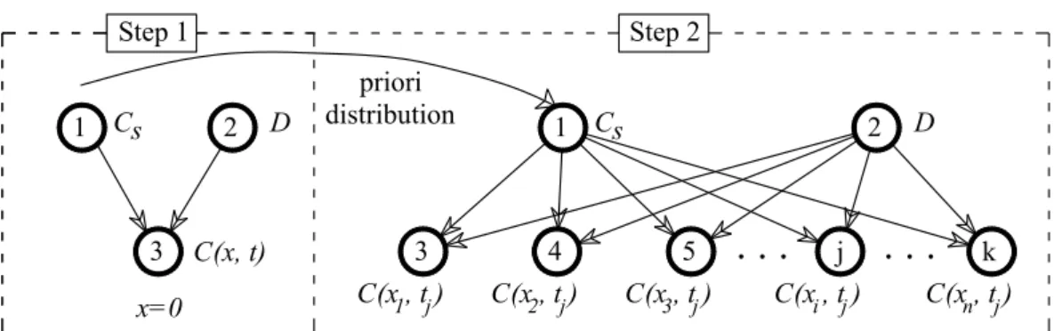
3.2.2. BN configurations and 2-steps identification procedure

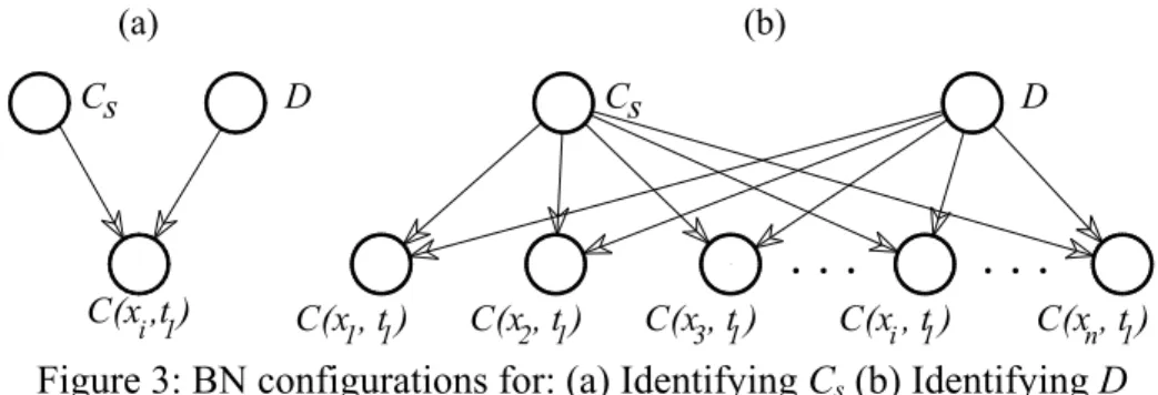
Parameter identification using BN is a complex problem that requires an improved configuration to reduce identification errors. Due to physical and model characteristics, Tran et al. [27] found that there are BN configurations that reduce the identification errors for each parameter. Inspection data near the surface is more valuable than those in the deeper part for identifying Cs. Therefore, the BN configuration with one child

node representing for chloride content at the concrete surface (x≈0) (Figure 3a) is used for the identification of Cs. The one-point-at-surface BN configuration includes also a

parent node D because in real conditions Cs cannot be determined at x=0 and then Cs

and D are dependent. For example, from a practical point-of-view the coring technique used to determine a chloride content estimates an average chloride value for the grinding depth dg (dg=0.3cm) at the average depth x=0.15cm. In addition, Cs at x ≈ 0 is

largely influenced by the exposure (rain, wetting and drying cycles, wind, etc.) under unsaturated conditions. Therefore taking a single measurement of Cs at x=0.15cm could

induce larger errors when wetting or drying processes modify the value of Cs at the

inspection time because a convection zone could appear. In this case, it will be more useful to use data from a point close to concrete surface but out of the effect of convection zone to identify Cs. This aspect is not illustrated in this study because it

requires real experimental data.

The use of a single BN that uses several points in depth (Figure 3b) generates additional errors for the identification of Cs. Figure 4 illustrates this point by comparing

the a posteriori histograms of Cs obtained from one-point-at-surface (Figure 3a) and

several points (Figure 3b). It is clear that the one-point-at-surface configuration provides results closer to the theoretical histogram.

For D, it is necessary to use the information from the total inspection length (L) to provide a better characterisation of the kinetics of the chloride ingress process. The BN configuration in such a case consists of several child nodes corresponding to chloride content at selected depth points derived from the discretisation of the total inspection length (Figure 3b). In the experimental procedure to determine chloride profiles, coring technique is used to determine an average chloride content in each grinding depth (slice). An average chloride content is determined from the powder extracted from each slice. The grinding depth (dg) was selected according to the accuracy of the

(10)

semi-9

destructive equipment and in this study, dg=0.3cm. Afterwards, it is possible to select

several inspection points corresponding to discretisation length (Δx) for updating the BN (Figure 5). Tran et al. [27] also pointed out that there is an optimal discretisation size for each inspection time. This means that there is an improved configuration for each analysed case corresponding to a discretisation that reduces the identification errors for the parameter D. Moreover, to reduce the level of uncertainty, Tran et al. [27] proposed a 2-steps identification procedure (Figure 6) where the used the a posteriori histogram of Cs obtained with one depth point configuration (step 1) as a priori

information for the estimation of D by considering several inspection points of BN configuration (step 2). This 2-steps procedure is used herein to improve the identification of D. Results in section 3.3.1 will illustrate this point.

3.3. Results

As previously mentioned in section 3.2, the BN configuration using one child node close to the surface is used for identifying Cs. However, for D, it is necessary to use the

BN with several child nodes representing for several measurements in depth to obtain a better identification. This section focuses on finding an optimal number of inspection points in depth representing an improved BN configuration to identify D using the 2-steps procedure described in section 3.2. Various BNs with different number of inspection points are considered to compare the identification errors. For a single inspection time nt = 1 and n = nx where the number of inspection points varies from n =

2 to n = nmax. n = 2 represents the case in which only two inspections points are

considered placed at the surface and at the total inspection depth (L) – i.e., x1 = 0 cm

and x2 = L. The maximum number of points nmax for a single inspection corresponds to

the case in which the minimum experimental discretisation size (∆x = 0.3 cm) is used. Figure 5 shows an intermediate case where L = 12 cm, nt = 1, and ∆x = 2 cm. For this

case n = nx = L/Δx + 1= 7 inspection points in depth.

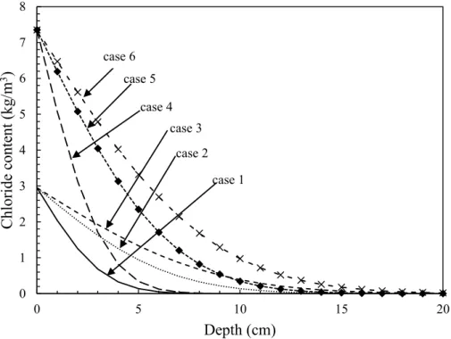
A single inspection time (nt = 1) at tins = 10 years was considered for all the cases.

The total inspection length of each case was defined based on the mean chloride profile (Figure 7) to cover all the potential chloride presence. Figure 7 was estimated from the mean values provided in Table 1 and tins = 10 years. The values of L and nmax for the 6

study cases are shown in Table 2.

3.3.1. Identification errors for D and influence of the discretisation size

Figure 8 depicts the estimated errors for the parameter D for a high level of aggressiveness and moderate concrete quality (case 2) as a function of the number of inspection points in depth, nx. Case 2 is selected because it appears frequently in

practice. For generalisation purposes, we considered a case with a larger number of evidences (10,000 chloride profiles). For comparative purposes, Figure 8 also includes results from a single BN configuration that considers the information from the total depth (Figure 3b).

In general, identification errors of statistical moments of D are smaller for the 2-steps procedure. This is due to the fact that considering a one-point-at-surface BN configuration in step 1 improves the identification of Cs and the second step is then

more useful for identifying D. Hence, the identification of D is now performed based on the 2-steps procedure. It can be seen that using more inspection points could not guarantee a better identification for the mean of D. The errors for the mean are close to 2% with nx > 4 (Figure 8a). However, for the estimation of the standard deviation, it is

(11)

10

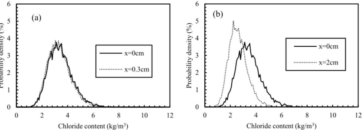
Figure 8b shows an increasing trend when nx > 13. This is mainly related to the

discretisation size Δx that decreases for larger values of nx – i.e., nx = L/Δx + 1. Figure 9

presents the probability densities of the evidences of the chloride content for two values of ∆x generated from the theoretical values (Table 1). In general, to obtain a good identification of D, the value of ∆x should be small to provide sufficient information about chloride profiles in depth. However, when ∆x is very small, the chloride content is almost the same between the two adjacent points. Therefore, the probability densities of the evidences used for updating in BN are very similar for two adjacent inspection points (Figure 9) and this will increase the identification errors. In contrast, when ∆x increases (x = 0cm and x = 2cm), the probability densities of the evidences are more different by reducing the identification errors (Figure 9). When ∆x is larger than the optimal value, the identification errors increase because the information becomes poor for describing the chloride ingress process [27]. Therefore, we will focus on the assessment of the optimal value of that minimises the identification errors for the standard deviation.

3.3.2. Optimal number of inspection points per depth for the different study cases

On the basis of the results presented in Figure 8, it is possible to find optimal ranges of

nx for given allowable identification error levels defined by decision makers. For

example, a decision maker can define allowable identification errors smaller than 10% and 20% for the identification of the mean and the standard deviation of D, respectively. Within this range, the value of nx that minimises the identification error of the standard

deviation is defined as an optimal value (nx,opt). For case 2, the optimal range is (8 – 15)

and the optimal number of inspection points is nx,opt = 8. The results for all considered

cases are summarised in Table 4. In fact, these ranges in real practice cannot ensure the same identification errors as we defined in theory (10% and 20% for the mean and standard deviation respectively) because there are many uncertainty involved in the problem that will vary for each application. However, they can be seen as recommendations to reduce the identification errors in real cases.

It is worth noticing that nx,opt is larger for RC structures with better concrete quality

under the same exposure condition. For example, the values of nopt for case 1, case 2

and case 3 are 19, 8 and 6 respectively, corresponding to good, ordinary and poor concrete quality. This phenomenon is related to the chloride diffusion coefficient for each concrete quality (Table 1). A chloride profile with a larger diffusion coefficient is characterised by a smaller slope in comparison to the other two cases (e.g, case 3, Figure 7). This means that the chloride content between the two adjacent inspection points is close (Figure 9). Therefore, the identification errors increase for a larger number of inspection points [27]. The identification results coming from BN with an optimal number of inspection points are used for the assessment of the probability of corrosion initiation in section 4.

4. Assessment of corrosion initiation risks from identified parameters

4.1. Probability of corrosion initiation

This section examines the effectiveness of improved BN configurations by using the identified data for the evaluation of the probability of corrosion initiation. The time to corrosion initiation, tini, is defined as the time at which the chloride concentration at the

(12)

11

chloride concentration for which the rust passive layer of steel is destroyed and the corrosion reaction begins. Cth depends on many parameters [5, 37, 42]: type and content

of cement, exposure conditions, time and type of exposure, distance to the sea, oxygen availability at the bar depth, type of steel, electrical potential of the bar surface, presence of air voids, definition of corrosion initiation, methods and techniques for measuring Cth, etc. Then, the determination of an appropriate Cth becomes a major

challenge for the owner/operator and it is therefore assumed that Cth is a random

variable. It was found convenient to propose three mean values of Cth depending on the

quality of concrete [37]. Table 1 contains the considered values for this random variable.

The corrosion initiation is calculated by evaluating the time-dependent variation of the chloride concentration at the reinforcing steel that is computed from Eq.(5). The limit state function that defines corrosion initiation can be written as:

( )

, _th

( )

_tc

( )

,

g X t =C X −C Xt (14)

where Ctc(X, t) is the total concentration of chlorides at the concrete cover depth c at

time t, function of the vector of random variables X. The probability of corrosion initiation, pini is obtained by integrating the joint probability function over the failure

domain g(X, t) ≤ 0 – i.e., Eq. (14). pini is estimated herein by using Monte Carlo

simulations.

4.2. Numerical example

4.2.1. Assessment of pini for case 2

We consider a RC component placed in a chloride-contaminated environment with high level of aggressiveness and ordinary quality concrete (case 2, Table 1). The BN configurations proposed in section 3 are used to identify both the mean and standard deviation of the parameters Cs and D by considering an optimal number of inspection

points in depth – i.e., nx,opt = 8 (Table 4). The identified parameters are then used in

Monte Carlo simulations to estimate the probability of corrosion initiation.

Figure 10 compares theoretical values with the predictions estimated from identified parameters when we have a large number of inspection data (10,000 numerical profiles) and when inspection data is limited (15 numerical profiles). It is clear that by using the improved configuration, the assessment of probability of corrosion initiation is close to the theoretical values even with 15 chloride profiles. The prediction errors with respect to theory described in Figure 10b reveal small errors excepting for the prediction at t=10 years. In fact, the probability of corrosion initiation at this time is relatively low (pini≈0.1) and therefore, more information is required to improve the accuracy at earlier

times. Consequently, for long-term predictions, this approach provides an acceptable assessment of pini.

4.2.2. Error for the assessment of pini in all studied cases

The errors on the assessment of probability of corrosion initiation with 15 chloride profiles for other cases reveal similar trends (Figure 11). The BN configurations used to identify both the mean and standard deviation of Cs and D consider the optimal number

of inspection points indicate in Table 4. The larger errors shown in Figure 11 are related with earlier times where the probability of corrosion initiation is smaller. When t > 40 years the errors are lower than 6% for only 15 chloride profiles. This work considered an inspection time of 10 years for all study cases. However, as mentioned in [24], for an

(13)

12

specific study case the error could be also reduced if other inspection times are considered. Optimal inspection times could be defined for each exposure and concrete quality.

5. Conclusions

Identification of parameters in chloride ingress models is an important task for predicting the level of chloride content penetrating into concrete. Inspection data used for identification is always limited due to time-consuming and expensive tests. Consequently, BN modelling of this phenomenon it considered herein for identifying random variables with a limited number of data in an optimal scheme. Based on a previous study about using BN for parameter identification [27], this study proposes an approach to select an optimal number of inspection points in depth that minimises the identification errors. The results obtained from different study cases indicated that the optimal number of inspection points in depth depends on both exposure and concrete quality. It was also found that the use of these optimal configurations improves the assessment of the probability of corrosion initiation. These findings can be used as recommendations for defining inspection schemes even if inspection data is limited.

Further work in this area will focus on the consideration of: • optimal inspection times for each study case,

• inspection costs, • real data,

• other deterioration models and,

• measurement errors and model uncertainty [17].

6. Acknowledgements

The ERDF funding of the European Union, program Interreg, for the project DurratiNet (2009-2012 Durable Transport Infrastructure in the Atlantic Area-Network), enabled us to undertake this study under good conditions. This work was co-founded by the SI3M project (2012-2016 Identification of Meta-Model for Maintenance Strategies) funded by Region Pays de la Loire (France). The authors of this paper would like to thank the Region Pays de la Loire (France) for its support to the SI3M project.

7. References

1. Lounis DZ, Amleh L (2003) Reliability-Based Prediction of Chloride Ingress and Reinforcement Corrosion of Aging Concrete Bridge Decks. In: Proceeding of the 3rd International IABMAS Workshop on Life-Cycle Cost Analysis and Design of Civil Infrastructure Systems. Lausanne, Switzerland, pp 139–147

2. Bastidas-Arteaga E, Bressolette P, Chateauneuf A, Sánchez-Silva M (2009) Probabilistic lifetime assessment of RC structures under coupled

corrosion-fatigue processes. Structural Safety 31:84–96. doi:

10.1016/j.strusafe.2008.04.001

3. Dang VH, François R (2013) Influence of long-term corrosion in chloride environment on mechanical behaviour of RC beam. Engineering Structures 48:558–568. doi: 10.1016/j.engstruct.2012.09.021

(14)

13

4. Sheils E, O’Connor A, Breysse D, et al. (2010) Development of a two stage inspection process for the assessment of deteriorating infrastructure. Reliability Engineering and System Safety 95:182–194.

5. Bastidas-Arteaga E, Schoefs F (2012) Stochastic improvement of inspection and maintenance of corroding reinforced concrete structures placed in unsaturated

environments. Engineering Structures 41:50–62. doi:

10.1016/j.engstruct.2012.03.011

6. Conciatori D, Grégoire É, Samson É, et al. (2014) Sensitivity of chloride ingress modelling in concrete to input parameter variability. Materials and Structures. doi: 10.1617/s11527-014-0374-8

7. Bastidas-Arteaga E, Schoefs F (2015) Sustainable Maintenance and Repair of RC Coastal Structures. Proceedings of the ICE - Maritime Engineering 168:162–173. doi: 10.1680/maen.14.00018

8. Torres-Luque M, Bastidas-Arteaga E, Schoefs F, et al. (2014) Non-destructive methods for measuring chloride ingress into concrete: State-of-the-art and future challenges. Construction and Building Materials 68:68–81. doi: 10.1016/j.conbuildmat.2014.06.009

9. Patil S, Karkare B, Goyal S (2014) Acoustic emission vis-à-vis electrochemical techniques for corrosion monitoring of reinforced concrete element. Construction and Building Materials 68:326–332. doi: 10.1016/j.conbuildmat.2014.06.068 10. du Plooy R, Villain G, Palma Lopes S, et al. (2013) Electromagnetic

non-destructive evaluation techniques for the monitoring of water and chloride ingress into concrete: a comparative study. Materials and Structures 48:369–386. doi: 10.1617/s11527-013-0189-z

11. Ploix M-A, Garnier V, Breysse D, Moysan J (2011) NDE data fusion to improve the evaluation of concrete structures. NDT & E International 44:442–448. doi: 10.1016/j.ndteint.2011.04.006

12. Lecieux Y, Schoefs F, Bonnet S, et al. (2015) Quantification and uncertainty analysis of a structural monitoring device: detection of chloride in concrete using DC electrical resistivity measurement. Nondestructive Testing and Evaluation 1– 17. doi: 10.1080/10589759.2015.1029476

13. Bastidas-Arteaga E, Chateauneuf A, Sánchez-Silva M, et al. (2011) A comprehensive probabilistic model of chloride ingress in unsaturated concrete. Engineering Structures 33:720–730. doi: 10.1016/j.engstruct.2010.11.008

14. Saassouh B, Lounis Z (2012) Probabilistic modeling of chloride-induced corrosion in concrete structures using first- and second-order reliability methods.

Cement and Concrete Composites 34:1082–1093. doi:

10.1016/j.cemconcomp.2012.05.001

15. Deby F, Carcasses M, Sellier A (2008) Toward a probabilistic design of reinforced concrete durability: application to a marine environment. Materials and Structures 42:1379–1391. doi: 10.1617/s11527-008-9457-8

16. Bastidas-Arteaga E, Schoefs F, Stewart MG, Wang X (2013) Influence of global warming on durability of corroding RC structures: A probabilistic approach. Engineering Structures 51:259–266. doi: 10.1016/j.engstruct.2013.01.006

(15)

14

17. Sheils E, O’Connor A, Schoefs F, Breysse D (2012) Investigation of the effect of the quality of inspection techniques on the optimal inspection interval for structures. Structure and Infrastructure Engineering 8:557–568. doi: 10.1080/15732479.2010.505377

18. O’Connor A, Kenshel O (2013) Experimental Evaluation of the Scale of Fluctuation for Spatial Variability Modeling of Chloride-Induced Reinforced Concrete Corrosion. Journal Of Bridge Engineering 18:3–14.

19. Peng L, Stewart MG (2014) Spatial time-dependent reliability analysis of corrosion damage to RC structures with climate change. Magazine of Concrete Research 66:1154–1169. doi: 10.1680/macr.14.00098

20. Giannini R, Sguerri L, Paolacci F, Alessandri S (2014) Assessment of concrete strength combining direct and NDT measures via Bayesian inference. Engineering Structures 64:68–77. doi: 10.1016/j.engstruct.2014.01.036

21. Pan Z, Chen A, Ruan X (2015) Spatial variability of chloride and its influence on thickness of concrete cover: A two-dimensional mesoscopic numerical research. Engineering Structures 95:154–169. doi: 10.1016/j.engstruct.2015.03.061

22. Stewart MG, Mullard JA (2007) Spatial time-dependent reliability analysis of corrosion damage and the timing of first repair for RC structures. Engineering Structures 29:1457–1464. doi: 10.1016/j.engstruct.2006.09.004

23. Soize C (2010) Identification of high-dimension polynomial chaos expansions with random coefficients for non-Gaussian tensor-valued random fields using partial and limited experimental data. Computer Methods in Applied Mechanics and Engineering 199:2150–2164. doi: 10.1016/j.cma.2010.03.013

24. Bastidas-Arteaga E, Schoefs F, Bonnet S (2012) Bayesian identification of uncertainties in chloride ingress modeling into reinforced concrete structures. Third International Symposium on Life-Cycle Civil Engineering

25. Richard B, Adelaide L, Cremona C (2012) A Bayesian approach to estimate material properties from global statistical data. European Journal of Environmental and Civil Engineering 37–41.

26. Tran T-B, Bastidas-Arteaga E, Schoefs F, Bonnet S (2014) Bayesian updating for optimization of inspection schedules of chloride ingress into concrete. Proceeding of the 2nd International Symposium on Uncertainty Quantification and Stochastic Modeling

27. Tran TB, Bastidas-Arteaga E, Schoefs F (2015) Improved Bayesian network configurations for probabilistic identification of degradation mechanisms: application to chloride ingress. Structure and Infrastructure Engineering 1–15. doi: 10.1080/15732479.2015.1086387

28. Finn VJ, Nielsson TD (2007) Bayesian Networks and Decision Graphs, Second

Edi. Journal of Chemical Information and Modeling. doi:

10.1017/CBO9781107415324.004

29. Tuutti K (1982) Corrosion of steel in concrete. Swedish Cement and Concrete Institute

(16)

15

of climate adaptation strategies for design of new concrete structures subject to chloride-induced corrosion. Structural Safety 52:40–53. doi: 10.1016/j.strusafe.2014.10.005

31. Meijers SJH, Bijen JMJM, de Borst R, Fraaij ALA (2005) Computational results of a model for chloride ingress in concrete including convection, drying-wetting cycles and carbonation. Materials and Structures 38:145–154. doi: 10.1007/BF02479339

32. Flint M, Michel A, Billington SL, Geiker MR (2013) Influence of temporal resolution and processing of exposure data on modeling of chloride ingress and reinforcement corrosion in concrete. Materials and Structures 47:729–748. doi: 10.1617/s11527-013-0091-8

33. Straub D (2009) Stochastic Modeling of Deterioration Processes through Dynamic Bayesian Networks. Journal of Engineering Mechanics 135:1089–1099. 34. Bensi MT, Der Kiureghian A, Straub D (2011) A Bayesian Network Methodology for Infrastructure Seismic Risk Assessment and Decision Support. University of California, Berkeley

35. Nguyen XS (2007) Algorithmes probabilistes appliqués à la mécanique des ouvrages de génie civil. PhD Thesis, INSA de Toulouse

36. Schoefs F, Boéro J, Clément A, Capra B (2012) The αδ method for modelling expert judgement and combination of non-destructive testing tools in risk-based inspection context: application to marine structures. Structure and Infrastructure Engineering 8:531–543. doi: 10.1080/15732479.2010.505374

37. Duprat F (2007) Reliability of RC beams under chloride-ingress. Construction and Building Materials 21:1605–1616.

38. Duracrete (2000) Probabilistic calculations. DuraCrete—probabilistic performance based durability design of concrete structures. EU—brite EuRam III. Contract BRPR-CT95-0132. Project BE95-1347/R12-13.

39. Vu KAT, Stewart MG (2000) Structural reliability of concrete bridges including improved chloride-induced corrosion. Structural Safety 22:313–333.

40. Cao Z, Wang Y (2014) Bayesian model comparison and selection of spatial correlation functions for soil parameters. Structural Safety. doi: 10.1016/j.strusafe.2013.06.003

41. Robinson JW, Hartemink AJ (2010) Learning Non-Stationary Dynamic Bayesian Networks. The Journal of Machine Learning Research 11:3647–3680.

42. Boubitsas D, Tang L (2014) The influence of reinforcement steel surface condition on initiation of chloride induced corrosion. Materials and Structures 48:2641–2658. doi: 10.1617/s11527-014-0343-2

(17)

16

List of Tables

Table 1: Probabilistic models of the variables ... 17

Table 2: Description of the considered study cases, inspection depths and maximum inspection points per case ... 17

Table 3: Discretisation of nodes and priori distribution ... 18

Table 4: Optimal values of inspection points for the 6 study cases ... 18

List of Figures Figure 1: A simple Bayesian network ... 19

Figure 2: General BN configuration for modelling chloride ingress ... 19

Figure 3: BN configurations for: (a) Identifying Cs (b) Identifying D ... 20

Figure 4: Comparison of theoretical histogram of Cs with a posteriori histograms obtained from one-point-at-surface and several points in depth BNs. ... 20

Figure 5: Spatial discretisation of chloride ingress measurements ... 21

Figure 6: Two-step procedure for improving identification with limited data ... 21

Figure 7: Mean chloride profiles for the 6 study cases at t=10 years ... 22

Figure 8: Error in identification of D for the case 2: (a) Mean, (b) Standard deviation . 22 Figure 9: Effect of discretisation size ∆x on the distribution of chloride content: (a) ∆x=0.3 cm – (b) ∆x=2 cm ... 23

Figure 10: (a) Probability of corrosion initiation – (b) Prediction error for pini ... 23

(18)

17

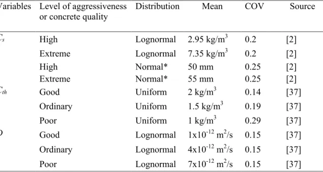
Table 1: Probabilistic models of the variables Variables Level of aggressiveness

or concrete quality Distribution Mean COV Source

Cs High Lognormal 2.95 kg/m3 0.2 [2] Extreme Lognormal 7.35 kg/m3 0.2 [2] c High Normal* 50 mm 0.25 [2] Extreme Normal* 55 mm 0.25 [2] Cth Good Uniform 2 kg/m3 0.14 [37] Ordinary Uniform 1.5 kg/m3 0.19 [37] Poor Uniform 1 kg/m3 0.29 [37] D _Good _{Lognormal 1x10}-12_m2_{/s 0.15} _[37] Ordinary Lognormal 4x10-12 m2/s 0.15 [37] Poor Lognormal 7x10-12_m2_{/s 0.15} _[37]

*Truncated at 10mm (lower bound)

Table 2: Description of the considered study cases, inspection depths and maximum inspection points per case

Case Level of aggressiveness Concrete quality Inspection depth L (cm) nmax

1 High Good 9 31 2 High Ordinary 15 51 3 High Poor 20 67 4 Extreme Good 9 31 5 Extreme Ordinary 15 51 6 Extreme Poor 20 67

(19)

18

Table 3: Discretisation of nodes and priori distribution

Parameters Number of states per

node, Ns

Priori distribution Range

Cs (kg/m3) 50 Uniform [0.5; 17] D (10-12 m2/s) 50 Uniform [0,1; 20]

C(xi, t) (kg/m3) 50 -a variable b

a _{Computed from a priori information of parent nodes} b _{Estimated as a function of the inspection depth}

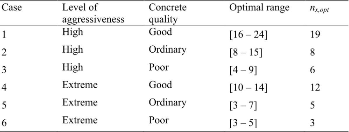
Table 4: Optimal values of inspection points for the 6 study cases

Case Level of

aggressiveness

Concrete quality

Optimal range nx,opt

1 High Good [16 – 24] 19 2 High Ordinary [8 – 15] 8 3 High Poor [4 – 9] 6 4 Extreme Good [10 – 14] 12 5 Extreme Ordinary [3 – 7] 5 6 Extreme Poor [3 – 5] 3

(20)

19

Figure 1: A simple Bayesian network

Figure 2: General BN configuration for modelling chloride ingress

X₂ X₃ X₁ 12 3 ... i ... 50 Range Pro bability densi ty N_s Cs D C(x , t )₁ ₁ C(x , t )₂ ₁ C(x , t )_{i 1} C(x , t )_{n 1} C(x , t )_{1 j} C(x , t )_{2 j} C(x , t )_i _j C(x , t )_{n j} C(x , t )_{1 m} C(x , t )_{2 m} C(x , t )_{i m} C(x , t )_{n m} . . . . . . . . . . . . . . . . . .

(21)

20

Figure 3: BN configurations for: (a) Identifying Cs (b) Identifying D

Figure 4: Comparison of theoretical histogram of Cs with a posteriori histograms

obtained from one-point-at-surface and several points in depth BNs.

(a) (b) Cs D C(x ,t )_{i 1} Cs D C(x , t )₁ C(x , t )₂ C(x , t )₃ C(x , t )_i C(x , t )_n . . . . . . 1 1 1 1 1 0 5 10 15 20 25 30 35 40 0.83 2.48 4.13 5.78 7.43 9.08 P ro bab ilit y den sity ( %) Chloride content (kg/m3₎

Histogram from one-point-at-surface BN Histogram from several points in depth BN Theoretical histogram

(22)

21

Figure 5: Spatial discretisation of chloride ingress measurements

Figure 6: Two-step procedure for improving identification with limited data

2 4 6 8 10 12

depth x (cm) C(x,t)

0

Δx=2cm

Total inspection depth=12 cm

d g=0.3cm 1 Cs 2 D 3 C(x, t) x=0 1 Cs 2 D 3 C(x , t )₁ 4 C(x , t )₂ 5 C(x , t )₃ j C(x , t )_i k C(x , t )_n . . . . . . j j j j j priori distribution Step 1 Step 2

(23)

22

Figure 7: Mean chloride profiles for the 6 study cases at t=10 years

Figure 8: Error in identification of D for the case 2: (a) Mean, (b) Standard deviation

0 1 2 3 4 5 6 7 8 0 5 10 15 20 Chloride c onte nt ( kg /m 3 ) Depth (cm) case 5 case 4 case 3 case 2 case 1 case 6 0 5 10 15 20 25 0 10 20 30 40 50 60 Er ror (% )

Number of inspection points From 2-steps procedure From 1 step (a) 0 50 100 150 200 250 0 10 20 30 40 50 60 Er ror (% )

Number of inspection points From 2-steps procedure From 1 step

(24)

23

Figure 9: Effect of discretisation size ∆x on the distribution of chloride content: (a) ∆x=0.3 cm – (b) ∆x=2 cm

Figure 10: (a) Probability of corrosion initiation – (b) Prediction error for pini

Figure 11: Errors on assessment of probability of corrosion initiation 0 1 2 3 4 5 6 0 2 4 6 8 10 12 Pr ob ab ili ty d en si ty ( %) Chloride content (kg/m3₎ x=0cm x=0.3cm 0 1 2 3 4 5 6 0 2 4 6 8 10 12 Pr ob ab ili ty d en si ty ( %) Chloride content (kg/m3₎ x=0cm x=2cm (a) (b) 0 0.1 0.2 0.3 0.4 0.5 0.6 0.7 0.8 0.9 1 0 20 40 60 80 100 Proba bili ty of c or rosion initiation Time (year) Theory 10000 profiles 15 profiles (a) 0 2 4 6 8 10 12 14 0 20 40 60 80 100 Err or (% ) Time (year) 10000 profiles 15 profiles (b) 0 2 4 6 8 10 12 14 0 20 40 60 80 100 Er ror (% ) Time (year) Case 1 Case 2 Case 3 Case 4 Case 5 Case 6