Bayesian nonparametric latent variable models

(1)

Bayesian Nonparametric Latent Variable Models

Thèse Patrick Dallaire Doctorat en informatique Philosophiæ doctor (Ph.D.) Québec, Canada © Patrick Dallaire, 2016

(2)

(3)

Résumé

L’un des problèmes importants en apprentissage automatique est de déterminer la com-plexité du modèle à apprendre. Une trop grande comcom-plexité mène au surapprentissage, ce qui correspond à trouver des structures qui n’existent pas réellement dans les don-nées, tandis qu’une trop faible complexité mène au sous-apprentissage, c’est-à-dire que l’expressivité du modèle est insuffisante pour capturer l’ensemble des structures présentes dans les données. Pour certains modèles probabilistes, la complexité du modèle se tra-duit par l’introduction d’une ou plusieurs variables cachées dont le rôle est d’expliquer le processus génératif des données. Il existe diverses approches permettant d’identifier le nombre approprié de variables cachées d’un modèle. Cette thèse s’intéresse aux méthodes Bayésiennes nonparamétriques permettant de déterminer le nombre de variables cachées à utiliser ainsi que leur dimensionnalité.

La popularisation des statistiques Bayésiennes nonparamétriques au sein de la commu-nauté de l’apprentissage automatique est assez récente. Leur principal attrait vient du fait qu’elles offrent des modèles hautement flexibles et dont la complexité s’ajuste pro-portionnellement à la quantité de données disponibles. Au cours des dernières années, la recherche sur les méthodes d’apprentissage Bayésiennes nonparamétriques a porté sur trois aspects principaux : la construction de nouveaux modèles, le développement d’algo-rithmes d’inférence et les applications. Cette thèse présente nos contributions à ces trois sujets de recherches dans le contexte d’apprentissage de modèles à variables cachées. Dans un premier temps, nous introduisons le Pitman-Yor process mixture of Gaussians, un modèle permettant l’apprentissage de mélanges infinis de Gaussiennes. Nous présen-tons aussi un algorithme d’inférence permettant de découvrir les composantes cachées du modèle que nous évaluons sur deux applications concrètes de robotique. Nos résultats dé-montrent que l’approche proposée surpasse en performance et en flexibilité les approches classiques d’apprentissage.

Dans un deuxième temps, nous proposons l’extended cascading Indian buffet process, un modèle servant de distribution de probabilité a priori sur l’espace des graphes dirigés acycliques. Dans le contexte de réseaux Bayésien, ce prior permet d’identifier à la fois la présence de variables cachées et la structure du réseau parmi celles-ci. Un algorithme d’in-férence Monte Carlo par chaîne de Markov est utilisé pour l’évaluation sur des problèmes d’identification de structures et d’estimation de densités.

Dans un dernier temps, nous proposons le Indian chefs process, un modèle plus géné-ral que l’extended cascading Indian buffet process servant à l’apprentissage de graphes et d’ordres. L’avantage du nouveau modèle est qu’il admet les connections entres les variables observables et qu’il prend en compte l’ordre des variables. Nous présentons un algorithme d’inférence Monte Carlo par chaîne de Markov avec saut réversible permettant l’appren-tissage conjoint de graphes et d’ordres. L’évaluation est faite sur des problèmes d’esti-mations de densité et de test d’indépendance. Ce modèle est le premier modèle Bayésien nonparamétrique permettant d’apprendre des réseaux Bayésiens disposant d’une structure complètement arbitraire.

(4)

(5)

Abstract

One of the important problems in machine learning is determining the complexity of the model to learn. Too much complexity leads to overfitting, which finds structures that do not actually exist in the data, while too low complexity leads to underfitting, which means that the expressiveness of the model is insufficient to capture all the structures present in the data. For some probabilistic models, the complexity depends on the introduction of one or more latent variables whose role is to explain the generative process of the data. There are various approaches to identify the appropriate number of latent variables of a model. This thesis covers various Bayesian nonparametric methods capable of determining the number of latent variables to be used and their dimensionality.

The popularization of Bayesian nonparametric statistics in the machine learning com-munity is fairly recent. Their main attraction is the fact that they offer highly flexible models and their complexity scales appropriately with the amount of available data. In recent years, research on Bayesian nonparametric learning methods have focused on three main aspects: the construction of new models, the development of inference algorithms and new applications. This thesis presents our contributions to these three topics of research in the context of learning latent variables models.

Firstly, we introduce the Pitman-Yor process mixture of Gaussians, a model for learning infinite mixtures of Gaussians. We also present an inference algorithm to discover the latent components of the model and we evaluate it on two practical robotics applications. Our results demonstrate that the proposed approach outperforms, both in performance and flexibility, the traditional learning approaches.

Secondly, we propose the extended cascading Indian buffet process, a Bayesian nonpara-metric probability distribution on the space of directed acyclic graphs. In the context of Bayesian networks, this prior is used to identify the presence of latent variables and the network structure among them. A Markov Chain Monte Carlo inference algorithm is presented and evaluated on structure identification problems and as well as density estimation problems.

Lastly, we propose the Indian chefs process, a model more general than the extended cascading Indian buffet process for learning graphs and orders. The advantage of the new model is that it accepts connections among observable variables and it takes into account the order of the variables. We also present a reversible jump Markov Chain Monte Carlo inference algorithm which jointly learns graphs and orders. Experiments are conducted on density estimation problems and testing independence hypotheses. This model is the first Bayesian nonparametric model capable of learning Bayesian learning networks with completely arbitrary graph structures.

(6)

(7)

List of Tables

3.1 MAP prediction success rates on five data sets Xj_test of unseen samples, with

the trained PYPMoG model. . . 61

3.2 Comparison of clustering accuracies between different unsupervised learning methods, for different time-window size W . . . . 65

3.3 Average terrain classification accuracy. . . 70

3.4 Leave-one-out averaged prediction accuracy . . . 74

4.1 Kullback-Leibler Divergence Estimations. . . 93

4.2 Posterior Means and Deviations on Structure Complexity . . . 95 5.1 Estimated Hellinger distance between fantasy datasets and the test set. The

(12)

(13)

List of Figures

2.1 Finite partitioning of the θ-space.. . . 16 2.2 An example of random discrete probability distribution generated from a

Dirich-let process with α = 10 and a uniform base distribution. The red sticks

repre-sent the probability of observing particular values of θ.. . . 17 2.3 The marginal probability of a Dirichlet process is a Dirichlet distribution.

The sequence shows that the Dirichlet process can be seen as the

infinite-dimensional generalization of the Dirichlet distribution. . . 19 2.4 Random matrices drawn from the Chinese restaurant process with different

values of α. The sampling starts from the bottom with the first customer, who is always assigned to table k = 1. The black blocks are representing the

customers choice of tables. . . 23 2.5 Illustration of Dirichlet process samples. The top row shows the stick-breaking

distribution and the bottom row transforms them into random probability dis-tributions. The solid line in the top row reflect the expected value of πk while

in the bottom row it corresponds to the normal distribution. . . 26 2.6 Random draws from the two-parameter stick-breaking distribution. The red

bars represent the first 50 weights {π_k}50

k=1. The blue curve is the cumulative

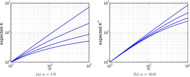
sum of weights showing the long tail behavior when d > 0. . . . 28 2.7 Expected value of K+ as a function of n in a log-log scale. The figures include

plots for d ∈ {0.0, 0.2, 0.5, 0.9}, respectively appearing from bottom to top in

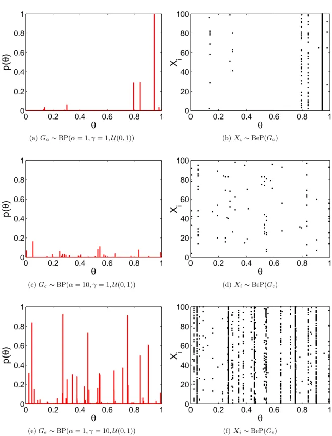
both figures. . . 30 2.8 Examples of random measures drawn from Beta processes with different

param-eters α and γ. Base distribution H is the uniform distribution U (0, 1). The left column shows the random measures we used to sample the Bernoulli processes

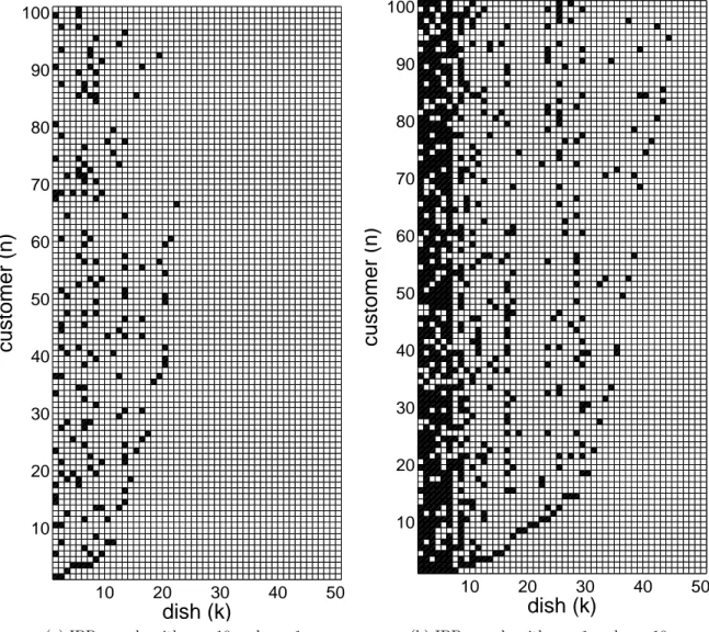
in the right column. . . 34 2.9 Examples of random binary matrices drawn from IBPs with different

parame-ters. The sampling starts from the bottom with the first customer. . . 36 3.1 Graphical model of the Pitman-Yor process mixture of Gaussians. The circular

nodes represent variables. When several variables have the same dependencies, we use the plate notation instead of repeating all variables with the same sub-graph. A plate generally looks like a rectangle containing indexed variables where the bottom-right symbol indicates the number of times the subgraph is

repeated. . . 48 3.2 Close-up view of the tactile probe, showing the steel pin and the triple axis

accelerometer (in red) attached near the tip. The leather-made attachment at

(14)

3.3 Turntable used to collect tactile probe data, with the tachometer measuring rotation velocity. The stack of discs, on the right, constitutes the surface test

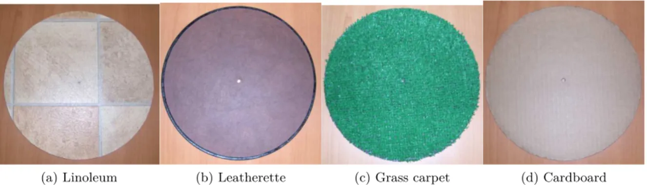
sets. . . 52 3.4 Picture of 4 discs used in the surface identification experiments. The complete

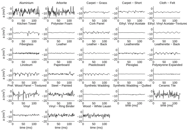
test set comprises 28 discs. . . 53 3.5 One time window of 100 samples for each of the 28 test surfaces. The signal is

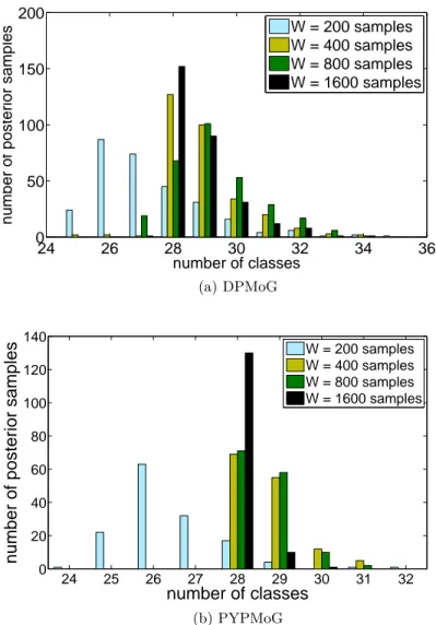
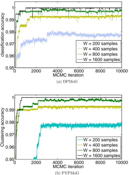
the acceleration in the Y direction only. . . . 54 3.6 Percentage of variance of the principal components. . . 57 3.7 Estimating the number of surfaces in an unlabeled data set. . . 58 3.8 Clustering accuracy on unlabeled data sets as a function of the MCMC

itera-tion, for different time window sizes W . For these experiments, the true number

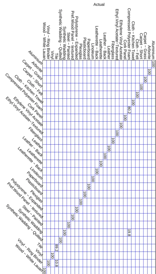
of clusters was unspecified. . . 59 3.9 Confusion matrix for the combined test set X1:5_test using time-window size of

W = 1600 samples. . . . 60

3.10 The expected posterior number of classes as a function of the training set size. All training sets contain the same number of examples for each surface. The blue solid line corresponds to the PYPMoG and the red dashed line is the

DPMoG. . . 62 3.11 Confusion matrix for test set XB using time-window size of W = 1600 samples. 63

3.12 The expected posterior clustering accuracy as a function the training set size. All training sets contain the same number of examples for each surface. The blue solid line corresponds to the PYPMoG and the red dashed line is the

DPMoG. . . 64 3.13 Histogram of the posterior on hyperparameter d obtained with MCMC. The

chain is computed with a data set of 50 examples per surface and with W = 1600. 64 3.14 TheMessor robot, used to collect the data sets in the experiments.. . . 66 3.15 Force/Torque signals registered with the foot-mounted sensor. Sub-figures are:

a) forces from concrete floor; b) torques from concrete floor; c) forces from sand; d) torques from sand. Each color denotes a signal axis: x-axis (red),

y-axis (green) and z-y-axis (blue). . . 68 3.16 Terrain samples used in the experiments: a) sand; b) green rubber; c) concrete

floor; d) PVC tiles; e) ceramic tiles; f) carpet tiles; g) artificial grass, h) grit; i)

pebbles; j) black rubber; k) wooden boards and l) rocks. . . 69 3.17 Confusion matrix of the maximum a posteriori PYPMoG. . . 70 3.18 Three non-overlapping Markov Chain Monte Carlo simulations on clustering

accuracy selected for visual assessment. . . 72 3.19 Histogram of the posterior distribution on pairwise correct classification when

training a PYPMoG for clustering terrains. . . 72 3.20 Posterior distribution on identified terrains. . . 73 4.1 Graphical representation of the information flow in the belief network. . . 79 4.2 Examples of several probability distributions representable with the nonlinear

Gaussian density function as a function of its parameters y and ρ. . . . 81 4.3 A random draw from the cascading Indian buffet process with K(0) = 3. The

binary matrices on the right come between the layers and indicate the existing connections. In this example, Z(5) is a zero-matrix, meaning that layer m = 5

(15)

4.4 Learning the directed acyclic graph in Fig. a) requires the CIBP to introduce

an extra node X to pass the message from A to C such as in Fig. b).. . . 87 4.5 A random draw from the extended cascading Indian buffet process showing

what the ECIBP provides. The gray arrows are taken from 4.3. On the right, binary matrices show the jumping connections only for layer m = 0 and its

grandparent layers. The matrices are finite dimensional in both dimensions. . . 88 4.6 The skeleton of the belief network to identify, where gray nodes are observable

and white nodes are hidden. . . 97 5.1 A practical example showing what are active nodes and inactive nodes. Given

that X is the only observable node, B is active because it is the parent of X and A is active for it is the parent of another active node. Node C is trivially inactive as it is not connected to any node. Being the child of an active node is not an activation element and therefore D is inactive. The same reasoning

applies for observable nodes, leaving E inactive.. . . 103 5.2 A directed acyclic graph augmented with order values and its adjacency matrix

representation. The labels of the graph respect the order values, making Z_AA a lower triangular binary matrix. The gray nodes represent observable variables

and white nodes are hidden variables. . . 107 5.3 Empirical study on the effect of hyperpameters α and γ. . . . 112 5.4 Empirical study of the model complexity as a function of the number of

ob-served variables. . . 113 5.5 The training sets showing the true distributions to learn. . . 116 5.6 Fantasy datasets produced by several posterior Bayesian networks. . . 117 5.7 Quadrimodal distribution generated with 2 independent bimodal distributions. 118 5.8 Results of learning from quadrimodal datasets of various sizes. . . 119 5.9 4 latent features used to generate the data sets. Each feature is composed of

0’s and 1’s as the color bars indicate. . . 121 5.10 4 latent features contained in the maximum a posteriori model. Those are closed

(16)

(17)

À ma mère Louisette, ma tante Fleurette ainsi que ma compagne Sandrine, les trois merveilleuses femmes qui ont permis que cette thèse se réalise dans la sérénité.

(18)

(19)

Remerciements

Tout d’abord, j’aimerais exprimer ma profonde gratitude envers Brahim Chaib-draa et Philippe Giguère, mes directeurs de recherches, pour les innombrables conseils qu’ils m’ont prodigués. Je les remercie de m’avoir écouté, de m’avoir guidé et de m’avoir motivé tout au long de ce parcours. Aussi, je les remercie de m’avoir fait confiance par rapport à mon choix de sujet de recherches et de m’avoir toujours laissé une grande liberté quant aux orientations à donner à mes recherches.

J’aimerais aussi remercier les membres du jury Claude-Guy Quimper, Nizar Bouguila, Thierry Duchesne, Philippe Giguère et Brahim Chaib-draa pour la correction de la thèse, les com-mentaires constructifs et les questions pertinentes.

Je remercie le Fonds québécois de la recherche sur la nature et les technologies (FQRNT) ainsi que mes directeurs pour le support financier. Cet aide m’a permis de me concentrer sur mon apprentissage et mon développement en tant que chercheur. Je remercie l’entreprise Yelp pour m’avoir offert un stage chez eux dans la magnifique ville de San Francisco.

Un merci spécial à Ludovic Trottier, un collaborateur et ami avec qui j’ai passé du temps exceptionnel. Nos nombreuses discussions sur des sujets farfelus ont très certainement été thérapeutiques. Je tiens aussi à remercier les membres du laboratoire DAMAS que j’ai côtoyés au cours de mes 10 années passées au sein du groupe. Un merci spécial à Camille Besse et Jean-Samuel Marier avec qui j’ai eu énormément de plaisir. Merci à Abdeslam Boularias, Andriy Burkov et Hamid Chinaei pour les excellentes discussions et les débats d’idées. Je vous remercie d’avoir influencé mes opinions, d’avoir ébranlé mes croyances et pour avoir partagé vos connaissances.

Finalement, une pensée très spéciale à ma famille. Le support de ma mère Louisette Dallaire et de ma tante Fleurette Dallaire a été indéniablement l’un des facteurs dominants de mon succès. Leur aide quotidienne m’a permis de me concentrer à temps plein sur mes recherches. Je remercie ma merveilleuse conjointe Sandrine Riopel pour sa patience, pour ses encouragements dans les moments difficiles et pour m’avoir accompagné à San Francisco. Son amour, son énergie et sa joie de vivre contagieuse me permettent de passer à travers n’importe quelle épreuve. Je remercie aussi Jonathan Duchesne pour avoir attentivement écouté mes théories

(20)

et pour ses nombreuses questions qui m’ont forcé à développer mes talents de vulgarisateur. Et Newton, pour sa naïveté, son envie de jouer et avoir égaillé ma vie tout simplement. À ma famille, je vous aime, merci de faire partie de ma vie.

(21)

Chapter 1

Introduction

Nowadays, artificial intelligence is everywhere. It is in our phones, cars, ATMs, video games and even assists physicians with medical diagnosis to only name a few. All these systems are specifically designed to replicate human cognitive abilities at different levels and can even surpass humans both on precision and in operation speed. This is a revolution: we now have the capacity to create artificially intelligent systems capable of making complex decisions through the application of sophisticated algorithms.

The most advanced techniques to produce artificially intelligent programs is to endow them with the ability to learn, i.e. allowing the program to improve its performance based on past experiences. Such an adaptive behavior is commonly seen in humans and animals, but is also present in some plants that are relying on sophisticated calcium-based signaling networks acting as their memory (Gagliano et al., 2014). The learning process of a program is not different: it requires information about its environment under the form of training examples and a way to memorize the current state of knowledge arising from experience.

Machine learning is the subfield of computer science studying learning algorithms. In general, learning tasks fall into one of three broad categories: supervised learning, unsupervised learn-ing or reinforcement learnlearn-ing. This categorization of the different learnlearn-ings can be related to the human nature. As children, we were being taught at school (supervised learning), we experienced the world by ourselves (unsupervised learning) and got grounded for misbehavior (reinforcement learning). The type of learning to employ depends on the nature of the task to accomplish. For instance, supervised learning aims to learn a function associating an input signal to an output signal while unsupervised learning only deals with input signals and seeks to discover the structures hidden into them. On the other hand, reinforcement learning is used when rewards signals are available after making sequences of decisions. When developing an intelligent system, it is important to carefully analyze the data in the first place so that we can decide on the appropriate type of learning to adopt.

(22)

fact, statistical learning has been observed in very young children for language acquisition and in object visual perception (Arciuli and Simpson, 2011). We can define statistical ma-chine learning as the application of the statistical learning methodology to mama-chine learning problems. The use of a statistical framework has several benefits. It allows rigorous analysis of the data, offers guarantees of convergence, gives confidence intervals on the results, etc. The recent successes of learning algorithms based upon statistics proved that statistical machine learning is not only a tool for theoretical analysis, but can truly be helpful in designing new algorithms for solving real-world problems.

Bayesian statistics constitute a large part of statistical machine learning (Gelman et al.,2014). A statistical framework based on the Bayesian paradigm exploits the laws of probability to represent current states of knowledge. Everything is formulated in terms of probability statements and the mathematics for updating the knowledge based on the data are well-described. This type of probabilistic machine learning is not restricted to learning a single model of the data. The observations can be consistent with several models and consequently determining which model is appropriate is also uncertain. The probability theory on which Bayesian methods build upon provides a framework for modeling this type of uncertainty. In Bayesian statistics, a model consists in specifying the joint distribution on all random variables describing the problem. Here, the role of the joint probability distribution is to encapsulate the variables’ interactions and their relative uncertainty. Different models will exhibit different interactions or even have varying number of variables when latent variables are allowed. One very flexible way of representing this is to use probabilistic graphical models, an approach relying on graphs for encoding conditional dependencies and independencies between all random variables appearing in the model. It has the advantage to compactly represent complex problems, such as real-world phenomena, and offers, through the use of graph theory, an effective way to address model complexity.

Graphical models (Lauritzen,1996) provide an intuitively appealing interface facilitating the modelization of highly-interacting sets of random variables and makes easier the visualization of the scope of each variable, including the variables that are not directly observed. Using this graph-based representation, efficient learning algorithms can be designed to infer latent variables by conditioning on the observables. The nature of the inference here is to estimate the hidden values taken by the latent variables given the realizations of the observed variables. When the model itself is also uncertain, i.e. that either the parameters associated with the distribution of the latent variables are unknown or the form of the distribution is unknown, the Bayesian framework becomes very useful as it can manage all this uncertainty related to what cannot be perceived.

Latent variables play an important role in machine learning (Bishop,2006). Many of the things we observe are influenced by causes we may not be able to see. For instance, when someone is

(23)

talking, the formulated sentence originates from specific thoughts that the speaker wants to communicate to the listener. The thoughts are obviously hidden and therefore they have to be inferred from a rather small number of words. Sometimes, a sentence might be ambiguous or even incomplete. This leads to inherent uncertainty on the listener’s side. Moreover, the number of possible thoughts is arguably infinite and makes this task even more challenging. Learning the dimensionality of latent variables is crucial for some machine learning problems. This is comparable to incrementally adding more thoughts to our repertoire as we grow up and listen to others trying to transmit these entirely new thoughts. Dimensionality can take various forms. Learning what values a random variable can take is one form, while identifying the number of latent variables present in a model is another. These problems are particular cases of structure learning in graphical models and are well-known to be difficult (Koller and Friedman,2009).

The general problem of structure learning aims to find the existing interactions between variables. For graphical models, this task translates into learning the graph that best factorizes the joint probability distribution of the variables. When all variables are known, although not necessarily observable, the number of potential graphs is finite, even though extremely large due to the combinatorial nature of graphs. An aspect of structure learning is identifying latent variables influencing the known variables. When the number of latent variables to introduce is unknown, this results in a potentially infinite number of graphical models to evaluate. In real-world problems it is common to suspect the presence of hidden cause while ignoring both their number and their scope of influence.

Bayesian nonparametrics offers an elegant statistical framework to the above-mentioned prob-lem of selecting a model having the right dimensionality (Hjort et al.,2009). The fundamental assumption of Bayesian nonparametrics is that models are all infinite dimensional. This, in a sense, eliminates all uncertainty about the model’s true dimensionality. However, Bayesian nonparametrics also assumes that for a finite amount of data, only a finite number of dimen-sions can manifest itself. This brings up the important question of determining which (active) dimensions were used to generate a particular dataset.

The number of dimensions allowed in a model is related to the complexity of the model. It turns out that Bayesian nonparametrics handles this by allowing the complexity of the model to grow appropriately with the amount of data, offering great flexibility during the learning phase. In the context of learning thoughts from spoken language, the Bayesian nonparametric paradigm would suggest that there exists an infinite number of thoughts in the world. With experience, a child would constantly hear new sentences. At the beginning, sentences are highly likely to convey entirely new thoughts. With experience, this probability decreases since most sentences can be associated to already known thoughts. Here, the learning paradigm assumes a constant evolution where more and more of the infinitely many thoughts are learned with

(24)

experience, but at some point, it becomes infrequent to encounter new thoughts.

This thesis focus on Bayesian nonparametric learning. Even though the field has engaged statisticians for about four decades, it only recently enjoyed a significant surge of interest. We ascribe this excitement to the enthusiasm of machine learning scientists towards highly flexible learning models and to the growth of available computational power. The two are intrinsically linked. Using highly flexible models can naturally lead to models of greater complexity which in turns requires a proportional amount of computational resources.

Current research on Bayesian nonparametric methods in machine learning focus on three important aspects:

1. constructing new models for dealing with different types of data; 2. designing efficient inference algorithms for the current models; and

3. developing new applications where Bayesian nonparametric methods are well-suited. In this thesis, we address all these points at different levels. However, the emphasis is placed on the development of new Bayesian nonparametric models for latent variable models. The last decade has been the scene of several new Bayesian nonparametric models. The In-dian buffet process is one seminal work in the field (Griffiths and Ghahramani,2006,2011). It opened the door to several latent factor learning methods such as the phylogenetic In-dian buffet process of Miller et al. (2012), the infinite factorial hidden Markov model of Gael et al.(2009) and the dyadic data model ofMeeds et al.(2006). A more practical appli-cation has recently been developed by Polatkan et al. (2015) which tackles the problem of super-images, the problem of recovering a high-resolution image from low-resolution images. Several new Bayesian nonparametric models are natural extensions or applications of the grandfather of Bayesian nonparametrics, the Dirichlet process (Ferguson,1973). For instance, Blei and Lafferty(2007) proposed a method to model topic correlations. InFox et al. (2011), the authors presented a Bayesian nonparametric approach for modeling systems with switch-ing linear dynamics. An infinite mixture of Gaussian processes was proposed byTayal et al.(2012) which allows finite decomposition of times series.Wood et al.(2011) developed the sequence memoizer, an algorithm learning Markov models with arbitrary orders and applied it to loss-less data compression.

1.1 Objectives

The objective of this thesis is to develop new machine learning methods based on Bayesian nonparametric statistics. As we stated before, Bayesian nonparametrics allows for more flexi-ble and more accurate learning procedure by scaling the complexity of the learned model with respect to the amount of available data. The motivation behind the development of these new

(25)

learning methods is to enlarge the current set of tools in machine learning with even more accurate learning methods.

The main question is: what model can we improve? There exists several models with im-provement potential. In this thesis, we are concerned with latent variable models and there will focus on improving current Bayesian nonparametric latent variable models. In the next section, we briefly describe the contributions of the thesis.

1.2 Contributions

In this thesis, we introduce novel models and present new applications of Bayesian nonpara-metrics to machine learning problems. All contributions belong to the broader field of com-puter science, although their impact touches several related fields of research such as robotics, probability & statistics and machine learning. In chronological order, our contributions are the following:

1. we introduce a clustering model based on the Pitman-Yor process for autonomous sur-face recognition. The main advantage of this model compared to traditional approaches is that it automatically learns the number of encountered surfaces. Once the learning is completed, the algorithm returns a set of potential clusterings reflecting the uncertainty about what surfaces are detected;

2. we introduce a supervised learning model based on the Pitman-Yor process for surface classification. The proposed model has the advantage of learning non-linear boundaries within the space of surfaces and also models the uncertainty of those boundaries. Since the model is learned with Bayesian methods, the algorithm can make probabilistic pre-dictions by returning full probability distributions over potential surfaces;

3. we present quantitative results for the cascading Indian buffet process. Previous works on the model only reported qualitative results, making it hard to assess the model efficiency on a practical problem. We evaluated the cascading Indian buffet process’ performance on learning graphical models in the context of density estimation;

4. we introduce an extended version of the cascading Indian buffet process allowing the learning of arbitrary directed acyclic graph structures within latent variables. This model is the first Bayesian nonparametric prior on such arbitrary structures where the number of nodes belonging to the graph is infinite. The new model has been applied to density estimation and structure identification problems;

5. we introduce the Indian chefs process, a Bayesian nonparametric prior on the joint space of directed acyclic graphs and orders. The advantage of this model over the extended cascading Indian buffet process is that observable nodes can now be interconnected. Moreover, this new prior allows inferring the order of the variables in the graph. We

(26)

applied the Indian chefs process model to density estimation problems, statistical inde-pendence tests and feature discovery; and

6. we develop an exact inference algorithm for the Indian chefs process. The algorithm is based on reversible jump Markov chain Monte Carlo methods where simulations visit the space of graphs and orders. The samplers composing the algorithm are designed in a way that they could be reused in other problems or to derive approximate inference approaches for the Indian chefs process.

1.3 Summary of Remaining Chapters

We now provide an overview of the chapters, including details of the methods used in each of them as well as descriptions of the experimental parts. We also briefly comment on the results and our conclusions.

Chapter 2: Background We begin with an introduction of the necessary concepts for a

good understanding of our contributions. This chapter, as well as the thesis, is highly focused towards probability and statistics. It is thus natural to start with a well-grounded motivation of Bayesian statistics from the machine learning perspective. We explain the learning me-chanics of Bayesian methods and discuss the role of the prior. The transition is made towards nonparametric Bayesian approaches. The chapter covers two of the most important priors in Bayesian nonparametrics, the Dirichlet process and Beta process. We discuss the theoretical aspects of these processes as well as models which can be derived from them. We conclude the chapter with an introduction to Markov chain Monte Carlo methods and conjugate models, two important practical tools to carry out posterior computation.

Chapter 3: Pitman-Yor Process Mixtures Applied to Surface Identification This

chapter presents an application of Bayesian nonparametric structure learning for the problem of surface identification. It first introduces the Pitman-Yor process mixture of Gaussians as a prior on infinite mixture of Gaussians exhibiting power-law behaviors. An inference algo-rithm for learning Gaussian mixtures is also presented. We then tackle the problem of surface recognition by describing a pre-processing approach for accelerometer signals originating from interactions with surfaces. The classification and clustering learning approaches derived from the Pitman-Yor process mixture of Gaussians are detailed and experiments are conducted with both learning algorithms. In our case, the experiments were done with an artificial fin-ger and a walking robot. Results demonstrated that our methods surpassed the predictive performance of the Pitman-Yor process mixture of Gaussians alternatives.

Chapter 4: The Extended Cascading Indian Buffet Process Structure learning in

(27)

chapter, we consider a specific kind of nonlinear Gaussian belief networks. We detail the parametrization of such networks and the generative process of the data. Then, we incre-mentally describe more and more complex Bayesian nonparametric priors on directed acyclic graph structures, thus relating previous works on this problem. Directed acyclic graphs are the most general structure representation for graphical models, which is the reason why we want to construct a prior supporting the whole space of graphs. The proposed prior, the extended cascading Indian process, achieves this goal of representing arbitrary graph structures within latent variables. We introduce an inference procedure for the proposed model and experiment it on low-dimensional data with strong data patterns. We also demonstrate that the model can perform structure identification by retrieving graphs from the correct class of equivalence.

Chapter 5: The Indian Chefs Process The extended cascading Indian buffet process

does not support graphs with connections among observable variables and forces all observ-ables to lie at the bottom of the structure. The Indian chefs process, which is the main con-tribution of this thesis, solves this problem. By truly supporting any possible directed acyclic graphs with any order and any number of latent variables, this Bayesian nonparametric model provides a way to perform exact structure inference in graphical models. The chapter includes a constructive definition of the Indian chefs process. A reversible jump Markov chain Monte Carlo sampler performing random walks on the space of graphs and orders is presented. This inference method sacrifices computational efficiency to the profit of exact inference. The rele-vancy of the proposed prior is demonstrated on several problems such as density estimation, independence testing and feature extraction.

Chapter6: Conclusion and Future Work We conclude with a retrospection on Bayesian

(28)

(29)

Chapter 2

Background

In this chapter, we introduce the necessary concepts for understanding latent variable models. A latent variable is a variable that cannot be observed or measured directly. It is thus natural to use the language of probability to quantify the intrinsic uncertainty of latent variables. For a Bayesian, conducting inference with a latent variable model corresponds to constructing and evaluating the posterior joint probability of all variables, both observable and latent. We elaborate on this concept by providing an introduction to Bayesian statistics, with a particular focus on nonparametric Bayesian methods. Finally, we introduce the standard strategies of inference required to understand how learning is performed in latent variables models.

2.1 The Bayesian Framework

The fundamental characteristic of the Bayesian methodology is to explicitly represent the uncertainty regarding the unknowns in a probabilistic language. Basically, everything is dealt with probabilities. Even statistical conclusions are made in terms of probability statements, which in principle facilitates a common-sense interpretation of the statistical results.

The flexibility and generality of the Bayesian framework endow it with the capacity to cope with complex problems. There is no theoretical limit to the complexity of the model, only practical ones. Models involving several parameters having complicated multilayered probabil-ity specifications can be easily represented from a Bayesian perspective. In practice, however, computational issues may arise when large models are specified. In such a scenario, one should take care of controlling the complexity of the model so that inference remains tractable or, at least, be computable in a reasonable amount of time.

A typical Bayesian analysis can be outlined as follows (with details in the next sections): — formulate a probability model for the data;

— express uncertainty about model parameters with probability distributions; — observe the data to construct the likelihood function; and

(30)

— perform posterior inference with Bayes’ theorem.

Once we have the posterior distribution, inferential questions can be answered through an appropriate analysis of the posterior.

The kind of questions we are looking to answer may differ depending on the type of prob-lems we are facing. From the machine learning point of view, supervised and unsupervised learning often require estimating model parameters to make predictions about future data, no matter how these parameters are learned, only the generalization performance of the model matters. On the other hand, in probability and statistics, hypothesis testing is a more fre-quent question and statisticians insist on proper and rigorous methodology. Nowadays, the Bayesian methodology is well accepted within the machine learning community and people are getting attracted by well-studied statistical frameworks such as the Bayesian paradigm. This has led to statistical machine learning. More recently, statistical learning has emerged as a new subfield of statistics, focusing on machine learning problems (such as unsupervised learning and supervised learning) with a strictly statistical scheme of thinking (James et al., 2013). This demonstrates the close relationship of machine learning and statistics as both are of substantial influence to each other.

In Bayesian data analysis, questions are answered by means of the posterior distribution. In what follows, we describe in more details the steps leading to so-called posterior and introduce the basic motivational arguments of the Bayesian paradigm.

2.1.1 The Likelihood Principle

There are three major schools of thought to statistical inference: Bayesian, Likelihoodism, and Frequentism (Gandenberger,2014;Sober,2002). Even though they have been in disagreement on many points for decades, all of them agree on one thing: the likelihood function, which is the result of combining the data and the probability model of the data.

Deciding on a probability model means choosing a probability distribution for the data. In a sense, its role is to link the parameters to the data, so that we can evaluate and compare different models for the same data. For instance, consider a set of n data points x₁, . . . , xn drawn independently from a unique random variable X having density function p(X | θ). The probability of these observations under this probability model is:

p(x1, . . . , xn| θ) = n

Y

i=1

p(xi| θ), (2.1)

where the joint probability is factorized due to the independence and identical distribution (iid) assumptions.

The likelihood function is a reinterpretation of Equation (2.1) as a function of the parameter where x1, . . . , xnare now known and fixed. Indeed, this function is used to evaluate the quality

(31)

of a specific probability model parametrized by θ by conditioning on the observations, which is denoted:

L(θ | x1, . . . , xn) = p(x1, . . . , xn| θ). (2.2)

Even though the likelihood function is constructed from a probability density function, it is not itself a probability density.

For a Frequentist, Equation (2.2) can be used to find the maximum likelihood estimator: ˆ

θ = arg max

θ

L(θ | x1, . . . , xn), (2.3)

along with confidence intervals around the estimated parameter.

For a Likelihoodist, Equation (2.2) is used to compare two hypotheses, such as parameters θ versus θ0, based on their likelihood ratio:

r = L(θ

0 _{| x}

1, . . . , xn) L(θ | x1, . . . , xn)

, (2.4)

where a likelihood ratio r > 1 is said to favor hypothesis θ0 as the true parameter while r < 1 values favor θ.

For a Bayesian, once the data have been observed, all the evidence relevant to the unknown parameter θ is considered encapsulated in the likelihood function. Basically, it means that the likelihood function contains everything we need to know from the data to perform Bayesian inference. This assumption is called the Likelihood Principle (LP) (Berger et al.,1988). The LP is implicit in Bayesian statistics while Frequentist methods, such as the p-value test, are known to violate it (Gandenberger,2014).

The likelihood function is one of two sources of information leading to the posterior distri-bution. In Section 2.1.3, we introduce the second source of information, namely the prior distribution, which is mandatory for Bayesian methods. Prior to this, in the next section, we motivate the use of prior distributions with the concept of exchangeability.

2.1.2 The Concept of Exchangeability

It is a common assumption to view a set of data as being generated by independent and identically distributed random variables. This assumption can be oversimplifying in many cases. On the opposite side, we have times series which assume that the data are generated from sequences of dependent random variables. This can again be a strong assumption. The exchangeability assumption can be seen as a compromise for many problems. It is less restrictive than iid and simpler than time series. What exchangeability states is that an infinite sequence of random variables x₁, x2, . . . is infinitely exchangeable if the joint probability of any finite subset x1, . . . , xn is invariant to any permutations. That is, it immediately follows

(32)

that:

p(x1, . . . , xn) = p(xπ(1), . . . , xπ(n)), (2.5)

where π is a permutation on a finite subset of random variables. This basically means that the order in which we observe the data does not matter. Given that the iid assumption holds, then infinite exchangeability follows immediately. However, the opposite is not always true since there exist exchangeable random variables that are statistically dependent. A typical example is the Pólya urn (Eggenberger and Pólya, 1923). It consists of an urn containing a few red and black balls. At time t, a ball is picked from the urn, defining xt, and is returned to the urn along with a second ball of the same color. Clearly, x_t+1 depends on the previous picks x₁, . . . , xt. However, there exists a distribution - the Beta distribution in the two-color case - which makes the picks exchangeable since the joint probability of the colors does not change under any permutation.

The exchangeability assumption is typically a reasonable assumption in machine learning and for statistical applications since it accurately describes a large class of experimental setups. Furthermore, the notion of exchangeability is fundamental to Bayesian statistics and has led to the celebrated de Finetti’s theorem (De Finetti, 1937). There are several reasons why this theorem is praised by Bayesians. The theorem, and its later generalizations (Bernardo and Smith,2009), have strong mathematical implications. It demonstrated tight connections between Bayesian and frequentist reasoning, it proved the existence of priors, it provided an interpretation of parameters which differs from what is usually accepted and it brought forth the Bayes’ Theorem and the Likelihood Principle as corollaries (Poirier,2010).

The formal definition of de Finetti’s theorem is the following. Assuming that x1, x2, . . . is an exchangeable sequence of real-valued random quantities, then the joint probability density of any finite subset x1, . . . , xnhas an integral representation of the form:

p(x1, . . . , xn) = Z Θ n Y i=1 p(xi | θ)p(θ)dθ. (2.6)

This representation entails that there exists a parametric probability model p(x | θ) gener-ating the data, i.e. the likelihood function, and, more importantly, there exists a probability distribution p(θ) - commonly called the de Finetti mixing distribution - which has to describe the initially available information about the parameter θ, i.e. the prior. Here, we must stress

thatthe existence of the prior distribution is not an assumption, but rather a direct conclusion

of the theorem. The prior on parameter space Θ can be interpreted as the belief about what the long-run relative frequency θ is when n → ∞.

2.1.3 Types of Prior Distributions

Bayesian methods are often criticized for their subjectivism and the main reason is the intrinsic nature of the prior distribution. One could argue that the choice of the probability model is

(33)

also subjective. For instance, assuming a linear regression model when high degree polynomials could fit well is a strong a priori knowledge injection. In machine learning, we often say that models are wrong, but some are useful. Under that premise, the prior distribution should be seen as such, another tool, just like the probability model of the data which might also be erroneous.

There are two opposing perspectives on how the prior should be chosen. These views sepa-rate Bayesians into two general categories, subjective Bayesians and objective Bayesians. In practice, most Bayesians lie in the gray area, applying whatever is punctually required. The subjective approach is based on the concept of belief and that a prior should reflect an opinion, a translation of knowledge into the probabilistic language. The uttermost form of this is prior elicitation (O’Hagan et al.,2006). This technique consists of interacting with domain experts to obtain their opinion, together with uncertainty, and to carefully formulate them into informative prior distributions. Since machine learning is mostly concerned with automatically learning algorithms, the idealized black box, this way of thinking is often unsustainable in practice.

The objective approach goes the other way around. The prior should not encapsulate im-portant knowledge, but rather be as non-informative as possible. Its role is to regularize the inference so that it goes in the right direction by bringing a minimal amount of information. This type of prior is often qualified as vague, non-informative or flat. The idea here is to let the data do the work. The simplest way of specifying a non-informative prior probability distribution is to assign equal probability to all elements. More sophisticated methods related to objective Bayesian inference include robust Bayesian analysis and nonparametric Bayesian analysis (Berger et al.,2006).

So far, we motivated the likelihood function and presented a theorem proving the existence of the prior. We now explain how Bayesian statistics make use of the two.

2.1.4 Bayesian Inference

In Bayesian statistics, inference is conducted through the computation of the posterior dis-tribution, which involves combining the likelihood function and the prior distribution with Bayes’ theorem: p(θ | x1, . . . , xn) = p(x1, . . . , xn| θ) p(θ) R Θp(x1, . . . , xn| θ) p(θ)dθ = p(x1, . . . , xn| θ) p(θ) p(x1, . . . , xn) , (2.7)

where p(θ | x₁, . . . , xn) is the posterior distribution over model parameter θ after observing data points x1, . . . , xn. Equation (2.7) can be seen as an update rule for beliefs which can either be applied to the full data set once or be applied sequentially one datum at a time where the posterior after the previous update becomes the prior for the next. The sequential updating is made possible by the conditional independence given parameter θ which allows factorizing

(34)

the likelihood function according to Equation (2.1) and thus decompose the Bayes’ rule. It is good to mention that, due to exchangeability, the order in which the data are supplied will not affect the end result as this will always produce identical posterior distributions.

One may notice that the denominator in Equation (2.7) corresponds to the integral represen-tation of de Finetti in Equation (2.6). This term is called the evidence or marginal likelihood and is the normalization constant of the posterior distribution. A common alternative form of Bayes’ rule omits this constant and is written as:

p(θ | x1, . . . , xn) ∝ p(x1, . . . , xn| θ) p(θ), (2.8)

which shows that the posterior distribution is in fact proportional to the joint probability of the observations and model parameters.

2.1.5 Making Predictions

As stated earlier, all inference is done by first computing the posterior. This is also true when the purpose of inference is making predictions about future observations. For instance, consider the case where we observe x1, . . . , xn and we want to predict the value of xn+1. To this end, we want to compute the posterior predictive distribution:

p(xn+1| x1, . . . , xn) =

Z

Θ

p(xn+1| θ) p(θ | x1, . . . , xn)dθ, (2.9)

which requires the posterior uncertainty about model parameters to be computed first. Then, for predictions, the uncertainty about the true parameters is taken into account by marginal-izing the data probability model with respect to the posterior on parameters.

It is important to point out that the predictions from Equation (2.9) are not point-estimates, but rather full distributions. A perfectly valid way of obtaining point-estimates, while re-specting the posterior predictive distribution, is to simply draw a random sample from it. In machine learning, predictions often come along with the notion ofloss function. The study of loss functions within the Bayesian framework refers to Bayesian decision theory (Berger, 2013); It is out of the scope of this thesis as we only deal with supervised and unsupervised learning problems.

Integrating over posterior models such as in Equation (2.9) can be difficult in practice. The main is reason is that integrals do not always lead to an analytical form. In such a case, the integration is carried out with numerical methods that might require lots of computation to get sufficiently good approximations of the exact distribution. One way to simplify predictions is to avoid the integral by using a single parametric model instead of considering them all. This technique is at the limit of the Bayesian philosophy because it does not take into account the uncertainty over parameters, but can perform well in practice if a good model is found. The most likely model under the posterior distribution:

ˆ

θ = arg max

θ

(35)

i.e. the maximum a posteriori (MAP) estimate, can fulfill this task. It is analog to the max-imum likelihood defined in Equation (2.3), but in the Bayesian framework, the prior now acts as a regularization term, a typical machine learning technique used to avoid overfit-ting (Schölkopf and Smola, 2002). Selecting a predictive model with this technique is in-tuitively more appealing than the straightforward maximum likelihood, especially from a machine learning perspective.

As we stated earlier, Bayesian nonparametric methods are well-known for their great flexibility and their automatic complexity scaling mechanisms for model selection. We now introduce the basics of Bayesian nonparametric methods.

2.2 Bayesian Nonparametrics

When using Bayesian methods, one wants to encapsulate the uncertainty about the model into the prior probability distribution. As more data get available, one would expect that the posterior distribution concentrates itself around the true model. However, this is under the assumption that the prior assigns non-zero probability to the true model, otherwise, identifying the model becomes impossible.

The support of the distribution (the set of elements having non-zero probability) is thus very important when specifying priors. For instance, when doing linear regression, one is actually assigning probability one to the linear model, setting aside all nonlinear models. When the true model happens to be nonlinear, it is going to receive probability 0 under the posterior because it is out of the prior’s support. Performing Bayesian inference in that context will lead to a concentration of the posterior probability in some neighborhood of the true model projected into this lower-dimensional space.

The idea behind the nonparametric Bayesian approach is to avoid situations where the true model is out of the support by enlarging it to the point it virtually contains all hypotheses. This is a Bayesian way of reflecting total ignorance about the dimensionality of the true model. However, there is one important assumption made by nonparametric approaches: we assume that the true model does not have any finite parametric representation. Keep in mind that the model can still infer parametric models via the concept of active parameters. The only constraint being to supply a finite amount of data examples. In other words, the model will always get more complex as more data become available, but will have a finite number of active parameters to explain what has been seen so far. We will come back several times on this concept and this will become clearer as we explain it for specific models.

In the next sections, we introduce two important stochastic processes for Bayesian nonpara-metric modeling, namely the Dirichlet process and the Beta process.

(36)

Figure 2.1 – Finite partitioning of the θ-space.

2.2.1 The Dirichlet Process

In its seminal paper, Ferguson (1973) proposed the first Bayesian nonparametric approach by demonstrating the existence of the Dirichlet process. This stochastic process is actually an extension of the common finite Dirichlet distribution to infinite-dimensional spaces. In what follows, we introduce the Dirichlet process, its marginalized version called theChinese

restaurant process and a construction of the Dirichlet process based upon the stick-breaking process.

2.2.1.1 Definition

The Dirichlet process (DP) is a probability distribution over discrete distributions. It has two parameters: a probability density function H defined on the parameter space Θ, which is called

thebase distribution, and a positive scalar α called the concentration parameter. We denote

by G ∼ DP(α, H) a Dirichlet process distribution on the space of probability distributions where G is a random discrete probability distribution with support in Θ.

Let us consider a finite partitioning {A1, . . . , AK} of space Θ respecting the following con-straints:

K

[

k=1

Ak= Θ Aj∩ Ak= ∅, j 6= k, (2.11)

where the disjoint union of the K subsets is the complete space such as in Figure 2.1. This represents the basic probability concept that each subset A_k is an event and its area corre-sponds to the probability of occurrence for that event. To obtain the probability of an event

Ak, one would simply integrate the probability distribution on this space with respect to this area. The measure-theoretic notation for this is to write G(A_k) to denote the probability of event Ak.

(37)

0 0.2 0.4 0.6 0.8 1 0 0.05 0.1 0.15 0.2 0.25 0.3 0.35 0.4 θ p( θ )

Figure 2.2 – An example of random discrete probability distribution generated from a Dirichlet process with α = 10 and a uniform base distribution. The red sticks represent the probability of observing particular values of θ.

Let us assume that G is a random probability distribution on Θ and is distributed according to a DP parametrized by H and α. By definition, the probability assigned by G to subset A_k, i.e. the measure G(A_k), is also a random variable since G is itself a random variable. More formally, a probability measure G is said to be Dirichlet process distributed if the measures of any finite partition follows a Dirichlet distribution, which we can express as:

(G(A1), . . . , G(AK)) ∼ Dir(αH(A1), . . . , αH(AK)), (2.12) where Dir(·) denotes the common finite Dirichlet distribution with K dimensions. What should be understood from Equation (2.12) is that the Dirichlet process has a Dirichlet distribution as its marginal distribution, hence the name Dirichlet process.

Intuitively, the Dirichlet process can be seen as assigning probabilities to functions. These functions are all defined on space Θ and can be interpreted as "floating" over the space depicted in Figure2.1. By integrating a function, say f , with respect to one of the subset A_k, i.e. computing integral R

θ∈Akf (θ), we obtain the probability of that particular event. Here,

functions are random and the partitioning can be done arbitrarily. The randomness of the functions creates uncertainty regarding the probability of discrete events. When letting the number of partitions go to infinity, something important happens. Not all subsets will receive positive probability, but only a finite number of them will. This will ultimately generate an infinite discrete probability distribution, where most outcomes have near 0 probability and only a few have significant probability to occur.

(38)

probabil-ity distribution drawn from a DP(10, U (0, 1)). The red bars correspond to the probabilprobabil-ity of atomic events. As we can see, only a few θ’s receive significant probability under this distribu-tion. The bars, together, form a function, i.e. a random probability measure. When evaluating the probability of bigger events such as in Figure2.1, we have to integrate this function. In Figure 2.3, we show several marginalizations of the Dirichlet process depicted in Figure 2.2. As the number of dimensions increases, the Dirichlet distribution gets closer to a Dirichlet process. This represents an intuitive construction of the Dirichlet process where each event can always be subdivided into 2 smaller events, up until there are infinitely many events and we obtain a Dirichlet process random sample.

The expectation and variance of the Dirichlet process are particularly enlightening about the effect of its parameters α and H. First, the expectation of a DP is solely determined by its base distribution H. In fact, for any measurable set A ⊂ Θ we have that:

E[G(A)] = H(A), (2.13)

which means that base distribution H serves as a prior guess on probability distribution G. The fact that H can be continuous and G discrete does not change anything. Another way of reading Equation (2.13) is that H(A) is the integral of probability density function H on area A and G(A) is an infinite sum of point masses within area A. Thus, base distribution

H determines the expected sum of point masses for an area A. Then, the uncertainty around

this last expectation depends on the concentration parameter α according to: V[G(A)] = H(A)(1 − H(A))

α + 1 , (2.14)

showing that increasing α results in a variance reduction, while near zero values translate into great uncertainty. When α → ∞, we also have that G(A) → H(A), leading to a DP having all of its probability mass concentrated on the base distribution H.

Equations (2.13) and (2.14) provide an overview of how the Dirichlet process distributes its probability mass in the space of probability distributions. This mass, however, can only be shifted within the space of discrete probability distributions. Even when the base distribution

H is set as a continuous distribution, the DP still assigns probability 1 to the subset of discrete

probability distributions. The stick-breaking construction, which we will introduce in Section 2.2.1.6, makes this property more explicit.

2.2.1.2 Posterior Distribution

An important result of Ferguson (1973) is an analytical form allowing simpler computation of posterior Dirichlet processes. The author found that, just like the standard Dirichlet dis-tribution, the Dirichlet process is conjugate to themultinomial likelihood.

To describe this posterior distribution, let us first assume a set of n independent and identically distributed observations θ1, . . . , θn drawn from an unknown distribution G. By specifying

(39)

0 0.2 0.4 0.6 0.8 1 0 0.2 0.4 0.6 0.8 θ p( θ )

(a) 2-dimensional marginal DP

0 0.2 0.4 0.6 0.8 1 0 0.2 0.4 0.6 θ p( θ ) (b) 4-dimensional marginal DP 0 0.2 0.4 0.6 0.8 1 0 0.2 0.4 0.6 θ p( θ ) (c) 8-dimensional marginal DP 0 0.2 0.4 0.6 0.8 1 0 0.2 0.4 0.6 θ p( θ ) (d) 16-dimensional marginal DP 0 0.2 0.4 0.6 0.8 1 0 0.2 0.4 0.6 θ p( θ )

(e) 32-dimensional marginal DP

0 0.2 0.4 0.6 0.8 1 0 0.2 0.4 0.6 θ p( θ ) (f) 64-dimensional marginal DP

Figure 2.3 – The marginal probability of a Dirichlet process is a Dirichlet distribution. The sequence shows that the Dirichlet process can be seen as the infinite-dimensional generalization of the Dirichlet distribution.

a prior G ∼ DP(α, H) on the unknown distribution, the posterior distribution given the observations becomes: G | θ1, . . . , θn∼ DP α + n, α α + nH + 1 α + n n X i=1 δθi ! , (2.15)

(40)

where δ_θ represents the unit mass centered on θ. Notice here that the posterior base distribu-tion is a weighted sum between the prior base distribudistribu-tion H and the empirical distribudistribu-tion:

1 n n X i=1 δθi. (2.16)

In this equation, α determines the importance of the prior base distribution in the posterior distribution. It will eventually be dominated by the empirical distribution when n α. The DP is therefore asymptotically consistent, since the posterior distribution converges towards the true distribution as the sample size n grows to infinity, granting it some Frequentist properties (Teh,2010).

From equations (2.13) and (2.15), we can deduce the expected posterior probability of any event A ⊂ Θ: E[G(A) | θ1, . . . , θn] = α α + nH(A) + 1 α + n n X i=1 δθi(A), (2.17)

where δ_θ returns 1 iff θ ∈ A. The behavior of this expectation, as the number of observations tends towards infinity, is given by:

lim n→∞E[G(A) | θ1, . . . , θn] = ∞ X k=1 πkδθk(A). (2.18)

Thus, we obtain a weighted sum of unit masses whose locations correspond to unique values {θ_k}∞_k=1contained in the set of observations and whose weights π_kare the empirical frequencies of the associated θk (Fox,2009).

2.2.1.3 Predictive Distribution

As we mentioned in Section 2.1.5, the need for making predictions is an important part of machine learning. Consider a random probability distribution G ∼ DP(α, H) for which we have a set of iid samples θ₁, . . . , θn. We want to determine the predictive distribution of θn+1 by marginalizing out the posterior distribution formulated in Equation (2.15). From Equation (2.17), we can compute the marginal posterior probability that θn+1∈ A. Thus, to obtain the predictive distribution, it is sufficient to reduce A ⊂ Θ to a singleton, which gives:

θn+1| θ1, . . . , θn∼ α α + nH + 1 α + n n X i=1 δθi. (2.19)

This expression corresponds to the base distribution of the posterior DP in Equation (2.15). In fact, the distribution obtained in Equation (2.19) is equivalent to drawing a ball from the generalized Pólya urn (Blackwell and MacQueen,1973).

2.2.1.4 The generalized Pólya urn

The Pólya urn (Eggenberger and Pólya,1923) is a metaphor describing multiple well-known discrete distributions with random sequences of colored balls drawn from an urn. Blackwell