Modelling dependency completion in sentence comprehension as a Bayesian hierarchical mixture process: A case study involving Chinese relative clauses

Modelling dependency completion in sentence comprehension

as a Bayesian hierarchical mixture process:

A case study involving Chinese relative clauses

Shravan Vasishth (vasishth@uni-potsdam.de)

Department of Linguistics, University of Potsdam, Germany.

Nicolas Chopin (nicolas.chopin@ensae.fr)

Ecole Nationale de la Statistique et de l’administration ´economique, Malakoff, France.

Robin Ryder (ryder@ceremade.dauphine.fr)

Centre de Recherche en Math´ematiques de la D´ecision, CNRS, UMR 7534, Universit´e Paris-Dauphine, PSL Research University, Paris, France.

Bruno Nicenboim (bruno.nicenboim@uni-potsdam.de)

Abstract

We present a case-study demonstrating the usefulness of Bayesian hierarchical mixture modelling for investigating cog-nitive processes. In sentence comprehension, it is widely as-sumed that the distance between linguistic co-dependents af-fects the latency of dependency resolution: the longer the distance, the longer the retrieval time (the distance-based ac-count). An alternative theory, direct-access, assumes that re-trieval times are a mixture of two distributions: one distribu-tion represents successful retrievals (these are independent of dependency distance) and the other represents an initial failure to retrieve the correct dependent, followed by a reanalysis that leads to successful retrieval. We implement both models as Bayesian hierarchical models and show that the direct-access model explains Chinese relative clause reading time data better than the distance account.

Keywords: Bayesian Hierarchical Finite Mixture Models; Psycholinguistics; Sentence Comprehension; Chinese Relative Clauses; Direct-Access Model; K-fold Cross-Validation

Introduction

Bayesian cognitive modelling (Lee & Wagenmakers, 2014), using probabilistic programming languages like JAGS (Plummer, 2012), is an important tool in cognitive science. We present a case study from sentence processing research showing how hierarchical mixture models can be profitably used to develop probabilistic models of cognitive processes. Although the case study concerns a specialized topic in psy-cholinguistics, the approach developed here will be of general interest to the cognitive science community.

In sentence comprehension research, dependency comple-tion is assumed by many theories to be a key event. For ex-ample, consider a sentence such as (1):

(1) a. The man (on the bench) was sleeping

In order to understand who was doing what, the noun The

manmust be recognized to be the subject of the verb phrase

was sleeping; this dependency is represented here as a di-rected arrow. One well-known proposal (Just & Carpenter, 1992), which we will call the distance account, is that depen-dency distance between linguistically related elements partly

determines comprehension difficulty as measured by read-ing times or question-response accuracy. For example, the Dependency Locality Theory (DLT) by Gibson (2000) and the cue-based retrieval account of Lewis and Vasishth (2005) both assume that the longer the distance between two co-dependents such as a subject and a verb, the greater the re-trieval difficulty at the moment of dependency completion. As shown in (1), the distance between co-dependents can in-crease if a phrase intervenes.

As another example, consider the self-paced reading study in Gibson and Wu (2013) in Chinese subject and object rel-ative clauses. The dependent variable here was the reading time at the head noun (official). As shown in (2), the dis-tance between the head noun and the gap it is coindexed with is larger in subject relatives compared to object relatives.1 Thus, the distance account predicts an object relative advan-tage. For simplicity, we operationalize distance here as the number of words intervening between the gap inside the rel-ative clause and the head noun. In the DLT, distance is op-erationalized as the number of (new) discourse referents in-tervening between two co-dependents; and in the cue-based retrieval model, distance is operationalized in terms of decay in working memory (i.e., time passing by).

(2) a. Subject relative [GAPi GAP yaoqing invite fuhao tycoon de] DE guanyuani official xinhuaibugui

have bad intentions

‘The official who invited the tycoon has bad in-tentions.

b. Object relative

1_{The dependency could be equally well be between the relative} clause verb and the head noun; nothing hinges on assuming a gap-head noun dependency.

[fuhao tycoon yaoqing invite GAPi GAP de] DE guanyuani official xinhuaibugui

have bad intentions

‘The official who the tycoon invited has bad in-tentions.

In the Gibson and Wu study, reading times were recorded using self-paced reading in the two conditions, with 37 sub-jects and 15 items, presented in a standard Latin square de-sign. The experiment originally had 16 items, but one item was removed in the published analysis due to a mistake in the item. We coded subject relatives as−1/2, and object relatives as+1/2; this implies that an overall object relative advantage would show a negative coefficient. In other words, an object relative advantage corresponds to a negative sign on the esti-mate.

The distance account’s predictions can be evaluated by fit-ting the hierarchical linear model shown in (1). Assume that (i) i indexes participants, i= 1, . . . , I and j indexes items,

j= 1, . . . , J; (ii) yi jis the reading time in milliseconds for the

i-th participant reading the j-th item; and (iii) the predictor X is sum-coded (±1/2), as explained above. Then, the data yi j

(reading times in milliseconds) are defined to be generated by the following model:

yi j= β0+ β1Xi j+ ui+ wj+ εi j (1)

where ui∼ Normal(0, σ2u), wj∼ Normal(0, σ2w) and εi j ∼

Normal(0, σ2

e); all three sources of variance are assumed to

be independent. The terms ui and wj are called varying

in-tercepts for participants and items respectively; they repre-sent by-subject and by-item adjustments to the fixed-effect interceptβ0. Their variances,σ2uandσ2wrepresent

between-participant (respectively item) variance.

This model is effectively a statement about the generative process that produced the data. If the distance account is cor-rect, we would expect to find evidence that the slope β1 is

negative; specifically, reading times for object relatives are expected to be shorter than those for subject relatives. As shown in Table 1, this prediction appears, at first sight, to be borne out. Subject relatives are estimated to be read 120 ms slower than object relatives, apparently consistent with the predictions of the distance account.

Estimate Std. Error t value ˆβ0 548.43 51.56 10.64*

ˆβ1 -120.39 48.01 -2.51*

Table 1: A linear mixed model using raw reading times in milliseconds as dependent variable, corresponding to the re-ported results in Gibson and Wu 2013. Statistical significance is shown by an asterisk.

The object relative advantage shown in Table 1 was

origi-nally presented in Gibson and Wu (2013) as a repeated mea-sures ANOVA.

To summarize, the conclusion from the above result would be that in Chinese, subject relatives are harder to process than object relatives because the gap inside the relative clause is more distant from the head noun in subject vs. object rela-tives. This makes it more difficult to complete the gap-head noun dependency in subject relatives. This distance-based ex-planation of processing difficulty is plausible given the con-siderable independent evidence from languages such as En-glish, German, Hindi, Persian and Russian that dependency distance can affect reading time (see review in Safavi, Hu-sain, and Vasishth (2016)).

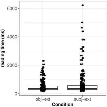
0 2000 4000 6000 obj−ext subj−ext Condition reading time (ms)

Figure 1: Boxplots showing the distribution of reading times by condition of the Gibson and Wu (2013) data.

However, the distributions of the reading times for the two conditions show an interesting asymmetry that cannot be straightforwardly explained by the distance account. At the head noun, the reading times in subject relatives are much more spread out than in object relatives. This is shown in Figure 1, where reading times are shown on the log scale. Although this spread was ignored in the original analysis, a standard response to heterogeneous variances (heteroscedas-ticity) is to delete “outliers” based on some criterion; a com-mon criterion is to delete all data lying beyond±2.5SD in each condition.2This procedure assumes that the data points identified as extreme are irrelevant to the question being in-vestigated. An alternative approach is to not delete data but to downweight the extreme values by applying a variance stabi-lizing transform (Box & Cox, 1964). Taking a log-transform 2_{In the published paper, Gibson and Wu (2013) did not delete} any data, leading to the results shown in Table 1.

of the reading time data, or a reciprocal transform, can re-duce the heterogeneity in variance; see Vasishth, Chen, Li, and Guo (2013) for analyses of the Gibson and Wu data us-ing a transformation.

One might think that if subject and object relatives are gen-erated by LogNormal distributions with different means, then modelling the data as being generated by LogNormals would adequately explain the data. Table 2 shows that if we assume such a model, there is no longer a statistically significant ob-ject relative advantage: the absolute t-value for the estimate of theβ1parameter is smaller than the critical value of 2 (Bates,

Maechler, Bolker, & Walker, 2015). Thus, assuming that the data are generated by LogNormal distributions with different means for the subject and object relatives leads to the conclu-sion that there isn’t much evidence for the distance account.

Estimate Std. Error t value

ˆβ0 6.06 0.07 92.64*

ˆβ1 -0.07 0.04 -1.61

Table 2: A linear mixed model using log reading times in mil-liseconds as dependent variable in the Gibson and Wu, 2013, data.

Consider next the possibility that the heteroscedasticity in subject and object relatives in the Gibson and Wu data reflects a systematic difference in the underlying generative processes of reading times in the two relative clause types. We investi-gate this question by modelling the extreme values as being generated from a mixture distribution.

Using the probabilistic programming language Stan (Stan Development Team, 2016), we show that a hierarchical mix-ture model provides a better fit to the data (in terms of predic-tive accuracy) than several simpler hierarchical models. As Nicenboim and Vasishth (2017) pointed out, the underlying generative process implied by a mixture model is consistent with the direct-access model of McElree, Foraker, and Dyer (2003). We therefore suggest that, at least for the Chinese relative clause data considered here, the direct-access model may be a better way to characterize the dependency resolution process than the distance account.

We can implement the direct-access model as a hierarchi-cal mixture model with retrieval time assumed to be generated from one of two distributions, where the proportion of trials in which a retrieval failure occurs (the mixing proportion) is

psrin subject relatives, and por in object relatives. The

ex-pectation here is the extreme values that are seen in subject relatives are due to psrbeing larger than por.

Subject relatives yi j∼psr· LogNormal(β + δ + ui+ wj, σ2e′) +(1 − psr) · LogNormal(β + ui+ wj, σ2e) Object relatives yi j∼por· LogNormal(β + δ + ui+ wj, σ2_e′) +(1 − por) · LogNormal(β + ui+ wj, σ2e) (2)

Here, the terms uiand wj have the same interpretation as in

equation 1.

Model comparison

Bayesian model comparison can be carried out using differ-ent methods. Here, we use Bayesian k-fold cross-validation as discussed in Vehtari, Gelman, and Gabry (2016). This method evaluates the predictive performance of alternative models, and models with different numbers of parameters can be compared (Vehtari, Ojanen, et al., 2012; Gelman, Hwang, & Vehtari, 2014).

The k-fold cross-validation algorithm is as follows: 1. Split data pseudo-randomly into K held-out sets y(k), where

k= 1, . . . , K that are a fraction of the original data, and K

training sets, y(−k). Here, we use K= 10, and the length of

the held-out data-vector y(k) is approximately 1/K-th the

size of the full data-set. We ensure that each participant’s data appears in the training set and contains an approxi-mately balanced number of data points for each condition. 2. Sample from the model using each of the K training sets, and obtain posterior distributions ppost(-k)(θ) = p(θ | y_(−k)), where θ is the vector of model parameters.

3. Each posterior distribution p(θ | y(−k)) is used to compute

predictive accuracy for each held-out data-point yi:

log p(yi| y(−k)) = log

Z

p(yi| θ)p(θ | y(−k)) dθ (3)

4. Given that the posterior distribution p(θ | y(−k)) is

summa-rized by s= 1, . . . , S simulations, i.e., θk,s_{, log predictive}

density for each data point yiin subset k is computed as

d el pd_i= log 1 S S

∑

5. Given that all the held-out data in the K subsets are yi,

where i= 1, . . . , n, we obtain the del pdfor all the held-out data points by summing up the del pd_i:

d el pd= n

∑

The difference between the del pd’s of two competing mod-els is a measure of relative predictive performance. We can also compute the standard deviation of the sampling distribu-tion (the standard error) of the difference in del pd using the formula discussed in Vehtari et al. (2016). Letting \ELPDbe the vector del pd₁, . . . , del pd_n, we can write:

se( del pd_m0− del pd_m1) = q

nVar( \ELPD) (6)

When we compare the model (1) with (2), if (2) has a higher del pd, then it has a better predictive performance com-pared to (1).

The quantity del pdis a Bayesian alternative to the Akaike Information Criterion (Akaike, 1974). Note that the relative complexity of the models to be compared is not relevant: the sole criterion here is out-of-sample predictive performance. As we discuss below (Results section), increasing complexity will not automatically lead to better predictive performance. See Vehtari et al. (2012); Gelman, Hwang, and Vehtari (2014) for further details.3

The data

The evaluation of these models was carried out using two sep-arate data-sets. The first was the original study from Gibson and Wu (2013) that was discussed in the introduction. The second study was a replication of the Gibson and Wu study that was published in Vasishth et al. (2013). This second study served the purpose of validating whether independent evidence can be found for the mixture model selected using the original Gibson and Wu data.

Results

In the models presented below, the dependent variable is read-ing time in milliseconds. Priors are defined for the model pa-rameters as follows. All standard deviations are constrained to be greater than 0 and have priors Cauchy(0, 2.5) (Gelman, Carlin, et al., 2014); probabilities have priors Beta(1, 1); and all coefficients (β parameters) have priors Cauchy(0, 2.5). Fake-data simulation for validating model Before evalu-ating relative model fit, we first simulated data from a mixture distribution with known parameter values, and then sampled from the models representing the distance account and the direct-access model. The goal of fake-data simulation was to validate the models and the model comparison method: with reference to the simulated data, we asked (a) whether the 95% credible intervals of the posterior distributions of the param-eters in the mixture model contain the true parameter values used to generate the data; and (b) whether k-fold cross valida-tion can identify the mixture model as the correct one when the underlying generative process matches the mixture model. 3_{We also used a simpler method than k-fold cross-validation} to compare the models; this method is described in Vehtari et al. (2016). The results are the same regardless of the model compari-son method used.

The answer to both questions was “yes”. This raises our con-fidence that the models can identify the underlying parame-ters with real data. The fake-data simulation also showed that when the true underlying generative process was consistent with the distance account but not the direct access model, the hierarchical linear model and the mixture model had com-parable predictive performance. In other words, the mixture model furnished a superior fit only when the true underlying generative process for the data was in fact a mixture process. Further details are omitted here due to lack of space.

The original Gibson and Wu study The estimates from the hierarchical linear model (equation 1) and the mixture model (equation 2) are shown in Tables 3 and 4. Note that in Bayesian modelling we are not interested in “statistical sig-nificance” here; rather, the goal is inference and comparing predictive performance of two competing models.

mean lower upper ˆβ1 6.06 5.91 6.20 ˆβ2 -0.07 -0.16 0.02 ˆ σe 0.52 0.49 0.55 ˆ σu 0.25 0.18 0.34 ˆ σw 0.20 0.12 0.33

Table 3: Posterior parameter estimates from the hierarchical linear model (equation 1) corresponding to the distance ac-count. The data are from Gibson and Wu, 2013. Shown are the mean and 95% credible intervals for each parameter.

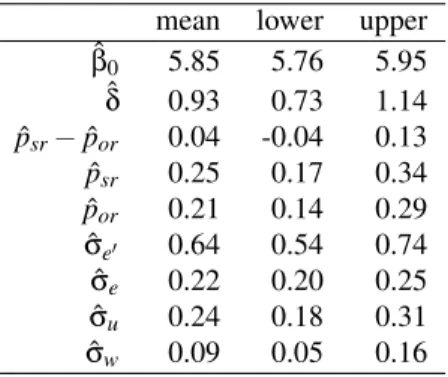
mean lower upper ˆβ0 5.85 5.76 5.95 ˆδ 0.93 0.73 1.14 ˆ psr− ˆpor 0.04 -0.04 0.13 ˆ psr 0.25 0.17 0.34 ˆ por 0.21 0.14 0.29 ˆ σe′ 0.64 0.54 0.74 ˆ σe 0.22 0.20 0.25 ˆ σu 0.24 0.18 0.31 ˆ σw 0.09 0.05 0.16

Table 4: Posterior parameter estimates from the hierarchi-cal mixture model (equation 2) corresponding to the direct-access model. The data are from Gibson and Wu, 2013. Shown are the mean and 95% credible intervals for each pa-rameter.

Table 4 shows that the mean difference between the prob-ability psr and por is 4%; the posterior probability of this

difference being greater than zero is 82%. K-fold cross-validation shows that del pd for the hierarchical model is −3761 (SE: 38) and for the mixture model is −3614 (35). The difference between the two del pds is 148 (18). The larger del pd in the hierarchical mixture model suggests that it has better predictive performance than the hierarchical

lin-ear model. In other words, the direct-access model has better predictive performance than the distance model.

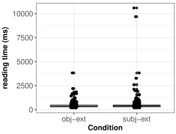
The replication of the Gibson and Wu study This data-set, originally reported by Vasishth et al. (2013), had 40 par-ticipants and the same 15 items as in Gibson and Wu’s data. Figure 2 shows the distribution of the data by condition; there seems to a similar skew as in the original study, although the spread is not as dramatic as in the original study.

0 2500 5000 7500 10000 obj−ext subj−ext Condition reading time (ms)

Figure 2: Boxplots showing the distribution of reading times by condition of the replication of the Gibson and Wu data.

Tables 5 and 6 show the estimates of the posterior distri-butions from the two models. Table 4 shows that the mean difference between the probability psrand poris 7%; the

pos-terior probability of this difference being greater than zero is 96%.

The del pdfor the hierarchical model is−3959 (53), and for the hierarchical mixture model,−3801 (38). The difference in del pdis 158 (29). Thus, in the replication data as well, the predictive performance of the mixture model is better than the hierarchical linear model.

mean lower upper ˆβ0 6.00 5.88 6.12 ˆβ1 -0.09 -0.16 -0.01 ˆ σe 0.44 0.41 0.47 ˆ σu 0.25 0.19 0.33 ˆ σw 0.16 0.10 0.26

Table 5: Posterior parameter estimates from the hierarchical linear model (equation 1) corresponding to the distance ac-count. The data are from the replication of Gibson and Wu, 2013 reported in Vasishth et al., 2013. Shown are the mean and 95% credible intervals for each parameter.

mean lower upper ˆβ0 5.86 5.78 5.95 ˆδ 0.75 0.56 0.97 ˆ psr− ˆpor 0.07 -0.01 0.15 ˆ psr 0.23 0.15 0.33 ˆ por 0.16 0.09 0.25 ˆ σe′ 0.69 0.59 0.81 ˆ σe 0.21 0.18 0.23 ˆ σu 0.22 0.17 0.29 ˆ σw 0.07 0.04 0.12

Table 6: Posterior parameter estimates from the hierarchical linear model (equation 2) corresponding to the direct-access model. The data are from the replication of Gibson and Wu, 2013 reported in Vasishth et al., 2013. Shown are the mean and 95% credible intervals for each parameter.

Discussion

The model comparison and parameter estimates presented above suggest that, at least as far as the Chinese relative clause data are concerned, a better way to characterize the de-pendency completion process is in terms of the direct-access model and not the distance account implied by Gibson and Wu (2013) and Lewis and Vasishth (2005). Specifically, there is suggestive evidence in the Gibson and Wu (2013) data that a higher proportion of retrieval failures occurred in subject relatives compared to object relatives. In other words, creased dependency distance may have the effect that it in-creases the proportion of retrieval failures (followed by re-analysis).4

There is one potential objection to the conclusion above. It would be important to obtain independent evidence as to which dependency was eventually created in each trial. This could be achieved by asking participants multiple-choice questions to find out which dependency they built in each trial. Although such data is not available for the present study, in other work (on number interference) (Nicenboim, Engel-mann, Suckow, & Vasishth, 2016) did collect this informa-tion. There, too, we found that the direct-access model best explains the data (Nicenboim & Vasishth, 2017). In future work on Chinese relatives, it would be helpful to carry out a similar study to determine which dependency was completed in each trial. In the present work, the modelling at least shows how the extreme values in subject relatives can be accounted for by assuming a two-mixture process.

Conclusion

The mixture models suggest that, in the specific case of Chi-nese relative clauses, increased processing difficulty in sub-ject relatives is not due to dependency distance leading to longer reading times, as suggested by Gibson and Wu (2013). 4_{A reviewer suggests that the direct-access model may simply} be an elaboration of the distance model. This is by definition not the case: direct access (i.e., distance-independent access) is incompati-ble with the distance account.

Rather, a more plausible explanation for these data is in terms of the direct-access model of McElree et al. (2003). Under this view, retrieval times are not affected by the distance be-tween co-dependents, but a higher proportion of retrieval fail-ures occur in subject relatives compared to object relatives. This leads to a mixture distribution in both subject and ob-ject relatives, but the proportion of the failure distribution is higher in subject relatives.

In conclusion, this paper serves as a case study demon-strating the flexibility of Bayesian cognitive modelling using finite mixture models. This kind of modelling approach can be used flexibly in many different research problems in cog-nitive science. One example is the above-mentioned work by Nicenboim and Vasishth (2017). Another example, also from sentence comprehension, is the evidence for feature overwrit-ing (Nairne, 1990) in parsoverwrit-ing (Vasishth, J¨ager, & Nicenboim, 2017).

Acknowledgments

We are very grateful to Ted Gibson for generously provid-ing the raw data and the experimental items from Gibson and Wu (2013). Thanks also go to Lena J¨ager for many insight-ful comments. Helpinsight-ful observations by Aki Vehtari are also gratefully acknowledged. For partial support of this research, we thank the Volkswagen Foundation through grant 89 953.

References

Akaike, H. (1974). A new look at the statistical model iden-tification. IEEE transactions on automatic control, 19(6), 716–723.

Bates, D., Maechler, M., Bolker, B., & Walker, S. (2015). Fitting linear mixed-effects models using lme4. Journal of

Statistical Software, 67, 1–48. doi: 10.18637/jss.v067.i01 Box, G. E., & Cox, D. R. (1964). An analysis of

transfor-mations. Journal of the Royal Statistical Society. Series B

(Methodological), 211–252.

Gelman, A., Carlin, J. B., Stern, H. S., Dunson, D. B., Ve-htari, A., & Rubin, D. B. (2014). Bayesian data analysis (Third ed.). Chapman and Hall/CRC.

Gelman, A., Hwang, J., & Vehtari, A. (2014). Understanding predictive information criteria for bayesian models.

Statis-tics and Computing, 24(6), 997–1016.

Gibson, E. (2000). Dependency locality theory: A distance-based theory of linguistic complexity. In A. Marantz, Y. Miyashita, & W. O’Neil (Eds.), Image, language, brain:

Papers from the first mind articulation project symposium.

Cambridge, MA: MIT Press.

Gibson, E., & Wu, H.-H. I. (2013). Processing Chinese rela-tive clauses in context. Language and Cognirela-tive Processes,

28(1-2), 125–155.

Just, M. A., & Carpenter, P. A. (1992). A capacity theory of comprehension: Individual differences in working mem-ory. Psychological Review, 99(1), 122–149.

Lee, M. D., & Wagenmakers, E.-J. (2014). Bayesian

cogni-tive modeling: A practical course. Cambridge University Press.

Lewis, R. L., & Vasishth, S. (2005). An activation-based model of sentence processing as skilled memory retrieval.

Cognitive Science, 29, 1–45.

McElree, B., Foraker, S., & Dyer, L. (2003). Memory struc-tures that subserve sentence comprehension. Journal of

Memory and Language, 48, 67–91.

Nairne, J. S. (1990). A feature model of immediate memory.

Memory & Cognition, 18(3), 251–269.

Nicenboim, B., Engelmann, F., Suckow, K., & Vasishth, S. (2016). Number interference in German: Evidence for

cue-based retrieval.Retrieved from https://osf.io/mmr7s/

(submitted to Cognitive Science)

Nicenboim, B., & Vasishth, S. (2017). Models of retrieval

in sentence comprehension: A computational evaluation

using Bayesian hierarchical modeling. Retrieved from

https://arxiv.org/abs/1612.04174 (Under revision following review, Journal of Memory and Language) Plummer, M. (2012). JAGS version 3.3.0 manual.

Interna-tional Agency for Research on Cancer. Lyon, France. Safavi, M. S., Husain, S., & Vasishth, S. (2016).

Depen-dency resolution difficulty increases with distance in Per-sian separable complex predicates: Implications for expec-tation and memory-based accounts. Frontiers in

Psychol-ogy, 7. doi: 10.3389/fpsyg.2016.00403

Stan Development Team. (2016). Stan modeling language users guide and reference manual, version 2.12 [Computer software manual]. Retrieved from http://mc-stan.org/

Vasishth, S., Chen, Z., Li, Q., & Guo, G. (2013, 10). Pro-cessing Chinese relative clauses: Evidence for the subject-relative advantage. PLoS ONE, 8(10), 1–14.

Vasishth, S., J¨ager, L. A., & Nicenboim, B. (2017). Feature overwriting as a finite mixture process: Ev-idence from comprehension data. In Proceedings of

MathPsych/ICCM. Warwick, UK. Retrieved from

https://arxiv.org/abs/1703.04081

Vehtari, A., Gelman, A., & Gabry, J. (2016). Practi-cal Bayesian model evaluation using leave-one-out cross-validation and WAIC. Statistics and Computing.

Vehtari, A., Ojanen, J., et al. (2012). A survey of bayesian predictive methods for model assessment, selection and comparison. Statistics Surveys, 6, 142–228.

Powered by TCPDF (www.tcpdf.org) Powered by TCPDF (www.tcpdf.org)