MODEL-BASED IMAGING APPROACH TO QUANTIFY TISSUE STRUCTURAL PROPERTIES IN OPTICAL COHERENCE TOMOGRAPHY

(1)

HAL Id: tel-01257509

https://tel.archives-ouvertes.fr/tel-01257509

Submitted on 23 Jan 2016

HAL is a multi-disciplinary open access archive for the deposit and dissemination of sci-entific research documents, whether they are pub-lished or not. The documents may come from teaching and research institutions in France or abroad, or from public or private research centers.

L’archive ouverte pluridisciplinaire HAL, est destinée au dépôt et à la diffusion de documents scientifiques de niveau recherche, publiés ou non, émanant des établissements d’enseignement et de recherche français ou étrangers, des laboratoires publics ou privés.

MODEL-BASED IMAGING APPROACH TO

QUANTIFY TISSUE STRUCTURAL PROPERTIES

IN OPTICAL COHERENCE TOMOGRAPHY

Cecilia Lantos

To cite this version:

Cecilia Lantos. MODEL-BASED IMAGING APPROACH TO QUANTIFY TISSUE STRUCTURAL PROPERTIES IN OPTICAL COHERENCE TOMOGRAPHY. Life Sciences [q-bio]. Université Paris Diderot, 2014. English. �tel-01257509�

(2)

1

UNIVERSITY PARIS DIDEROT - PARIS VII

Laboratory of Matter and Complex Systems

UNIVERSITY OF HOUSTON

Department of Mechanical Engineering

GRADUATE SCHOOL FRONTIERS IN LIFE SCIENCES, PARIS

PhD THESIS

Biomedical Engineering

Cecília LANTOS

MODEL-BASED IMAGING APPROACH TO

QUANTIFY TISSUE STRUCTURAL PROPERTIES

IN OPTICAL COHERENCE TOMOGRAPHY

Thesis directed by Stéphane DOUADY / Matthew A. FRANCHEK

Defended the September 29, 2014.

COMMITTEE

Mr. A. Claude BOCCARA

Reviewer

Mr. Stephen WONG

Reviewer

Mr. Matthew A. FRANCHEK

Thesis Director

Mr. Stéphane DOUADY

Thesis Director

Mrs. Darine ABI-HAIDAR

Examiner

(3)

2

UNIVERSITÉ PARIS DIDEROT - PARIS VII

Laboratoire Matière et Systèmes Complexes

UNIVERSITÉ DE HOUSTON

Département de l’Ingénierie Mécanique

ÉCOLE DOCTORALE FRONTIÈRES DU VIVANT, PARIS

THÈSE DE DOCTORAT

Ingénierie Biomédicale

Cecília LANTOS

QUANTIFICATION DE STRUCTURES

TISSULAIRES EN TOMOGRAPHIE PAR

COHÉRENCE OPTIQUE

Thèse dirigée par Stéphane DOUADY / Matthew A. FRANCHEK

Soutenue le 29 septembre 2014.

JURY

M. A. Claude BOCCARA

Rapporteur

M. Stephen WONG

Rapporteur

M. Matthew A. FRANCHEK

Directeur de thèse

M. Stéphane DOUADY

Directeur de thèse

Mme. Darine ABI-HAIDAR

Examinatrice

(4)

3

“For an image, since the reality after which it is modeled does not belong to it, and it exists ever as the fleeting shadow of some other, must be inferred to be in another [that is, in space], grasping existence in some way or other, or it could not be at all.”

(5)

4

Abstract

The dissertation presents a revolutionary method to tissue characterization. The optical scattering property of the tissue measured with Optical Coherence Tomography (OCT) reveals the subsurface structure at histological level. Our work developed a model based approach to process OCT data for accurate tissue characterization. This way the qualitative images are represented in a quantitative model independently from the measurement settings. Since a tumor is differentiated from healthy tissue based on morphological analysis, our parametric model is able to diagnose healthy versus cancerous tissue.

(6)

5

Résumé

Cette dissertation représente une méthode révolutionnaire pour la caractérisation du tissu. La propriété de diffusion optique du tissue mesurée en Tomographie par Cohérence Optique (OCT) révèle la structure tissulaire sous la surface à l’échelle histologique. Notre œuvre a développé une approche basée sur modèle pour traiter les données OCT pour la précise caractérisation du tissue. Ainsi les images qualitatives sont représentées dans un modèle quantitatif indépendamment de réglages de mesure. Etant donné qu’une tumeur est différenciée du tissu sain basé sur une analyse morphologique, notre modèle paramétrique est capable de diagnostiquer le tissu sain vs cancéreux.

(7)

6

Acknowledgement

I would like to thank my former academic advisors, Marc Durand and Patrice Flaud for giving me the opportunity to join their ranks at Paris Diderot University and start work on a highly interdisciplinary project in the Laboratory of Matter and Complex Systems. This, together with my integration in the laboratory and graduate school has given me the inspiration that allowed me to accomplish the project laid down in my PhD thesis. Many thanks also go out to the successive directors of the laboratory, Loïc Auvray and Jean-Marc di Meglio.

Next, I should like to express my to gratitude to François Taddéi, director of the Frontiers in Life Sciences International and Interdisciplinary Graduate School, for his scientific and personal support. This research report would not have been possible without his support, and that of his co-director, Samuel Bottani, who did all the administrative work required for the completion of my PhD work.

Many thanks are due to Stéphane Douady, my academic supervisor at Paris Diderot University, for supporting me in the new direction my thesis has taken within the scope of the international collaboration between the Laboratory of Matter and Complex systems and the University of Houston, where Matthew Franchek my academic mentor led me through the evolution of this work at the Mechanical Engineering Department. I am also grateful to the UH Mechanical Engineering chairman, Pradeep Sharma, for his wisdom and knowledge that helped me to achieve my PhD thesis.

Special thanks to Kirill Larin from the Department of Biomedical Engineering at the University of Houston who opened his laboratory to us to be able to work with Optical Coherence Tomography and to use their datasets measured on tissue samples supplied from collaboration with the MD Anderson Cancer Center.

I would like to thank the members of the research group I was involved when I began to work on my project. I could always rely on them for all kinds of support, from basic to elaborate. They helped me answer the many questions that arose while developing my ideas: Rafik Borji in System Identification and Control Engineering, then Narendran Sudheendran and Shang Wang in Optical Coherence Tomography.

This international collaboration could not have been realized without the support of the Hungarian-American Fulbright Committee, and the Department of Hydrodynamic Systems at the Budapest University of Technology and Economics. Beside the grant from the Paris Diderot University, and the Fulbright Committee, I obtained financial support from the University of Houston Foundation, the Frontiers in Life Sciences Graduate School, and Matthew Franchek’s sponsorship at the University of Houston.

My deepest gratitude is also due to the members of the supervisory committee for their valuable feedback in the defense, Laurent Limat, Darine Abi Haidar, Matthew Franchek, Stéphane Douady, and especially to my reviewers: Claude Boccara and Stephen Wong.

(8)

7

In Paris, I acknowledge the scientific and personal discussion and support with my friends and colleagues, Florence Gazeau, Nebraska Zambrano, and Kees van der Beek, and with my tutors Darine Abi Haidar and Dirk Drasdo.

I would like to dedicate all this work to my closest friend, Kees van der Beek who supported me during all of these years. He was not only a friend, he was also an advisor by scientific discussions, in writing papers, and giving presentations.

Special thanks also to my family and all my friends who have always been there for me, either they are in Houston (Patty, Judit, Fatemeh), Paris (Malak, Cecilia, Li, Camille, Zsuzsa) or Budapest (Edina, Judit, Mariann, Anna).

(9)

8

List of Figures

Figure I.1.1. Soft Tissue Development. MSC: Mesenchymal Stem Cell [2]. ... 22

Figure I.2.1. a) Adipocyte b) Adipose tissue with fibrous septa (dividing wall) between clusters of adipocytes. CT- Connective Tissue [33, 34]. ... 28

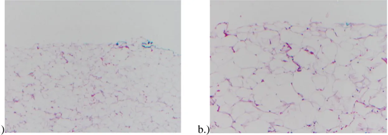
Figure I.2.2. Normal fatty tissue with large fat cells. Histology (H&E – hematoxylin & eosin stain). Magnification: a) 4x, b) 10x. ... 28

Figure I.2.3 Adipose tissue in reactive states. Medium magnification [9]. ... 29

Figure I.2.4. Atypical lipoma/lipoma-like WDLS M: 4-10x [11]. ... 30

Figure I.2.5. Atypical adipocytes in atypical lipoma/lipoma-like WDLS [11]. ... 30

Figure I.2.6. Stromal sclerosis in Atypical lipoma/lipoma-like, WDLS [11]. ... 30

Figure I.2.7. WDLS with myxoid features [11]. ... 30

Figure I.2.8. DDLS subtypes: a. Myxofibrosarcoma b. Solitary fibrous tumor c. Fibrosarcoma d. Gastrointestinal stromal tumor [11]. ... 31

Figure I.2.9. DDLS subtypes: a. Pleomorphic liposarcomatous component b. Mildly pleomorphic spindle cell sarcoma c. Pleomorphic component with large cells containing eosinophilic hyaline globules d. Osteosarcomatous differentiation [11]. ... 31

Figure I.2.10. X-ray of the abdomen with soft tissue tumor findings [36]. ... 32

Figure I.2.11. CT of LPS in the Retroperitoneum. ... 33

Figure I.2.12. a) T1 weighted- b) T2 weighted fat saturated axial MRI of a liposarcoma [7]. ... 33

Figure I.2.13. Doppler ultrasound on LS [7, 38]... 34

Figure I.2.14. Moderately hypervascular tumor in the right upper thigh [16]. ... 35

Figure I.2.15. Comparison of OCT image and Histology. ... 35

Figure I.2.16. FDG-PET/CT image of high grade soft tissue sarcoma in the right thigh with high FDG uptake (SUVmax, 18.4). [29]. ... 36

Figure I.2.17. Luciferase-labeled human Liposarcoma cells injected subcutaneously in SCID mice. Left mouse with the non-angiogenic dormant tumor undetectable by gross examination. Right mouse with developed angiogenic tumor after 133 days. The tumor is palpable ~23 days after well detectable bioluminescence signal [42]... 37

Figure I.2.18. Fluorescence images of Normal Fat Tissue, WDLS and DDLS. FISH analysis (Fluorescence in situ hybridization) Fluorophores: Centromeric probe (green), MDM2 probe (red), Dapi nuclear stain (blue). ... 37

Figure II.1.1. Electromagnetic spectrum [46]. ... 39

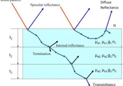
Figure II.1.2. Simplified model of biological medium with three layers. Each layer is associated with an absorption coefficient μa, a scattering coefficient μs , an anisotropic factor g, and a refractive index n [44]. ... 40

Figure II.1.3. Scheme of Confocal Microscopy [51]. ... 41

Figure II.1.4. Single- and Multi-photon excitation [49]. ... 41

Figure II.1.5. Dual-function reporter genes. One single protein with two functional components/ or coding sequences can be combined to make a single mRNA that produces two proteins [49]. ... 42

Figure II.1.6. Comparison of conventional imaging methods for diagnosis [69]. Ultrahigh Resolution OCT can achieve a resolution up to 1 µm. ... 44

(12)

11

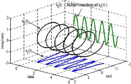
Figure II.2.1. Electro-magnetic wave propagation [81]. ... 47 Figure II.2.2. Solution of hyperbolic partial differential equation on space-time plane. ... 48 Figure II.2.3. Left: Monochromatic light (coherence length is infinity). Right: Broadband signal: Sum of the different wavelengths yields a wavepacket (Short Coherence Length Light) [modified from 59]. ... 50 Figure II.2.4. Optical Spectrum and Coherence Function of the Laser source: S840-B-I-20: 20 mW

Benchtop Lightsource at 840 nm. Left: Power Spectral Density in the function of wavenumber or

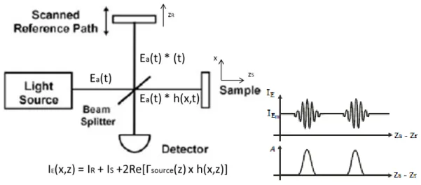
wavelength ( ), and Right: corresponding Point Spread Function of the generated Laser Signal; Up: High-Power Mode, Down: Low-Power Mode. ... 51 Figure II.2.5. Hilbert function of a single wavelength; Analytic signal represented in a 3D plot [87]. .... 53 Figure II.2.6. Broadband signal. The real high frequency signal a(t) is shown in black with the real envelope of its analytic signal A(t) in red [88]. ... 54 Figure II.3.1. Michelson Interferometer. Wave constructive/destructive interference appears on the detector due to path-length difference ( ) from the two mirrors (point source).

Interference fringe pattern appears in case of divergent laser source: ... 56 Figure II.3.2. Schematic of TD-OCT, IE - IEm = LCI signal, A is the real envelope [modified from 59 & 85]. ... 57 Figure II.3.3. Conventional OCT operation mode. Cross-sectional images (B-scan) are composed of adjacent A-lines [49]. ... 58 Figure II.3.4. Schematic of SD OCT with interference fringes detected on the camera array (I(k)) from one and two layers, with the backreflection (F(z)) after Fourier Transform [59, 85]. ... 58 Figure II.3.5. Schematic of SS OCT with interference fringes detected in time, and backreflection after Fourier Transform [59]. ... 59 Figure II.3.6. Scan planes of conventional OCT yielding cross-sections, and OCM yielding ‘en face’ images scanning laterally [89]. ... 60 Figure II.3.7. Parallel OCT detection [85]. ... 60 Figure II.3.8. Standard fiber-optic Michelson interferometer with 2:2 fiber coupler [92]. ... 61 Figure II.3.9. Free-space equivalent to the fiber-optic Michelson interferometer with a beamsplitter cube [92]. ... 61 Figure II.3.10. a-b) UHR OCT of macular hole in vivo c) Fundus photograph, white arrow shows central foveal region where OCT cross-section was recorded d) corresponding histology from similar postmortem eye [59]. ... 62 Figure II.3.11. a-c) Stained Histology of diseased human coronary arteries obtained autopsy and d-f) corresponding OCT images [59]. ... 63 Figure II.3.12. Optical therapeutic window [99]. ... 64 Figure II.3.13. OCT image penetration depth of human epiglottis ex vivo performed at 850-nm and 1300-nm central wavelengths penetrating deeper into the tissue, and corresponding histology; g –

glandular structure, c – cartilage. Bar equals 500 µm [49]. ... 64 Figure II.3.14. Free space OCT iso-resolution lines; Axial resolution vs. bandwidth of OCT light sources [100-102]. ... 65 Figure II.3.15. Normalized Optical Power Spectrum and Coherence Function of our OCT system. Laser source: Supraluminescent Diode (SLD) S840-B-I-20: 20 mW Benchtop Lightsource at 840 nm; a) Power Spectral Density and b) corresponding Point Spread Function. ... 67

(13)

12

Figure II.3.16. Optical spectrum using femtosecond Ti:Al2O3 laser with 260 nm linewidth and 1.5 µm axial resolution vs. a standard resolution SLD light source with 32 nm linewidth and 11.5 µm axial

resolution [59]. ... 68

Figure II.3.17. Comparison of different laser light sources representing the advantages of supercontinuum (SC) over amplified spontaneous emission (ASE), and superluminescent LED (SLD) [103, 108]. ... 68

Figure II.3.18. Ideal optical geometry. Numerical Aperture defined by the half-angle θ of the light cone angle, focused to point source F, f – focal length, d – lens diameter, n – refractive index of the medium. 69 Figure II.3.19. Diffraction of light through an aperture with D diameter [111]. ... 70

Figure II.3.0.20. Image formation of light with circular numerical aperture [112]. ... 70

Figure II.3.21. The depth of field is an inverse function of the Numerical Aperture. ... 71

Figure II.3.22. Comparison of OCT operating at low NA and OCM operating at high NA with overlapped coherence and confocal gate enhancing resolution and image quality, but at limited depth [modified from 114]. ... 72

Figure II.3.23. Gaussian beam intensity distribution [modified from: 122]. ... 74

Figure II.3.24. The propagation of a Gaussian beam [modified from 111 & 123]. ... 74

Figure II.3.25. Gaussian Laser beam profile, with parameters: beam waist (2w0), focal length, Depth of focus (b), Divergence angle (θ) [modified from 124]. ... 76

Figure II.4.1. SD-OCT measurement setup in the laboratory on a table against vibration... 80

Figure II.4.2. SD-OCT scheme [24]. ... 80

Figure II.4.3. Fourier Transform of the Interferometer Exit. ... 83

Figure II.4.4. Interferometer Exit recorded on Normal Fat Tissue. ... 84

Figure II.4.5. Normal Fat Tissue.a) OCT A-line (1mm = 228 px) b) B-scan composed of 100 A-lines (white bar = 500 µm). ... 85

Figure II.4.6. a) Autocorrelation for a perfectly balanced detector b) Phase delay (zeroth order) c) Group delay (first order) d) GVD (second order) [128]. ... 87

Figure II.4.7. Degradation of PSF (point spread function), peak broadening and intensity loss at increasing path-length differences without dispersion compensation (linear & logarithmic scale). ... 88

Figure II.4.0.8. Interferometer Exit; Spectrum from two interfered signals, one is delayed by a path-length-difference l = 400 µm; and chirped due to dispersion. ... 89

Figure II.4.9. a) Complex representation of the fringe signal b) Unwrapped phase. ... 90

Figure II.4.10. Point Spread Functions in function of path-length difference with dispersion compensation (linear & logarithmic scale). ... 90

Figure II.4.11. a) Simulated interferogram; Dotted line: light source spectrum G(ζ); Solid line: interferometric modulation; δζ: pixel width b) Fourier transform of the interferogram [136]. ... 91

Figure II.4.12. Scattering process and wavefront dispersion affecting OCT images [104]. ... 94

Figure III.1.1. Attenuation of backscattered light (red line) in tissue after averaging 500 A-lines. Tissue surface begins at around 1000 μm (Intensity on logarithmic scale). ... 95

Figure III.1.2. OCT image of the boundary between healthy tissue and DDLS. The left part of the image is the denser tumor area; the right part is the normal fat tissue containing adipose cells [26]. ... 96

Figure III.1.3. Threes curves show the backscattered intensity in time at three different positions in the sclera reduced from OCT measurements. The arrows show the diffusion starting point [143]. ... 96

(14)

13

Figure III.1.5. Averaged OCT profile with numerical fit to three layers: Red-Intima, Blue-Media, Green-Adventitia, logarithmic scale [141]. ... 99 Figure III.1.6. Averaged OCT A-scan (thin grey line), and the fitted signal using equation (III.1.7) (thick dark line) with the calculated attenuation coefficient µt (± 95% confidence interval) reduced from two

layers; logarithmic scale [151]. ... 99 Figure III.1.7. Involved (malignant) human axillary lymph node with diffuse involvement of the node tissue a) H&E histology b) parametric OCT image c) en face OCT image at a specific depth position; Scale bar = 1 mm [157]. ... 100 Figure III.1.8. OCT signal with slope, and after subtracting the slope from the raw A-scan, logarithmic scale [159]. ... 101 Figure III.1.9. Slope and standard deviation of Fat Tissue, WDLS, Smooth Muscle Connective Tissue and its cancerous version: Leiomyosarcoma. 40000 sample points per sample, and 1 sample per tissue type are represented with 95% confidence intervals [159]. ... 101 Figure III.1.10. (A) Photograph (B) Schematic of the Biopsy guidance probe [161]. ... 102 Figure III.1.11. OCT A-scan profiles of breast tissue specimens: (A) adipose; (B) fibroglandular tissue; and (C) adenocarcinoma recorded with Low-Coherence Interferometry. Insets are the histological sections [161]. ... 102 Figure III.1.12. OCT A-line from adipose (left) and fibroglandular (right) human breast tissue with first-order fit (red line); Logarithmic scale [162]. ... 103 Figure III.1.13. Averaged, area normalized power spectra on human adipose and fibroglandular tissue in breast, calculated from training set. Green window shows ROI [162]. ... 103 Figure III.1.14. Adipose, fibroglandular and tumor tissue characteristics in breast. Parameters of Slope, Standard Deviation around slope and Spatial Frequency are calculated from a training set. The last two parameters show similar characteristics [162]. ... 104 Figure III.1.15. OCT A-line a) Adipose tissue b) Inductive ductal carcinoma tumor tissue c) Stroma tissue; Logarithmic Scale [164]. ... 105 Figure III.1.16. Fourier-Domain data normalized by area, and averaged from tumor (black), stroma (dark gray), and adipose (light gray) tissue A-lines [164]. ... 106 Figure III.1.17. Histogram of the mean distance between high-intensity backreflections from 1 OCT A-line of human tumor (black), stroma (dark gray) and adipose (light gray) tissues [164]. ... 106 Figure III.1.18. Steps of A-line processing: first column – adipose tissue; second column – fibrous and adipose tissue; third column – tumor tissue; 8 parameters are extracted [163]. ... 108 Figure III.1.19. Scatter plot illustrating the clustering of the three main tissue types (adipose – green, fibrous – blue, tumor - red) and their projections on the x, y, and z planes for three parameters: Slope, Std, and PeakArea [163]. ... 109 Figure III.1.20. H&E images of adipose with stromal regions (a), cancer with adipose cells (d), and stroma (e), their corresponding OCT B-scans [(b)(e)(h)], and fractal dimension distribution calculated from the A-lines of the B-scan [(c)(f)(i)] [165]. ... 110 Figure III.1.21. a) A-scan profile selected from b) B-scan at porcine artery. Arrows show the

approximative region of intima (image size: 1.5 x 3 mm2); Logarithmic scale [141]. ... 111 Figure III.1.22. Example OCT images (after 4x4 local average filtering – better result) of mouse (a) skin, (b) fat, (c) normal lung and (d) abnormal lung. Image size: 1x0.25 mm [166]. ... 112 Figure III.1.23. a. OCT B-scan of Stratum Corneum (up) and Epidermis (down) segmented manually. b. Different fitting distributions to the B-scan data of Stratum corneum and Epidermis [168]. ... 113

(15)

14

Figure III.1.24. a) OCT image of chick embryo b) Spatial contrast computed from a 7x7 moving window

[169]. ... 114

Figure III.1.25. Original A-scan profile and similar A-scan at the end of the process recorded at two SD-OCT devices [172]. ... 115

Figure III.2.1. Histological images. ... 116

Figure III.2.2. Tissue Cross-Sections. OCT Images (B-scans composed of 500 A-lines); ... 117

Figure III.2.3. OCT A-line of Normal Fat Tissue a) arbitrary unit b) dB scale. ... 118

Figure III.2.4. OCT A-line of WDLS a) arbitrary unit b) dB scale. ... 118

Figure III.2.5. OCT A-line of DDLS a) arbitrary unit b) dB scale. ... 118

Figure III.2.6. 5 A-line-plots x = pixel position of the A-line from the B-scans of Figure III.2.2, and the mean value of 400 A-lines. A) Normal Fat Tissue b) WDLS (Well-Differentiated Liposarcoma) c) DDLS (De-Differentiated Liposarcoma) . ... 120

Figure III.2.7. Mean, standard deviation, and standard deviation over mean of 400 A-lines of the OCT images on Figure III.2.2. ... 120

Figure III.2.8. Intensity variation of 400 A-lines in a B-scan at specific depth positions z [pixel]. (1mm = 228 pixels) ... 121

Figure III.2.9. Reordered Intensity Values from Figure III.2.8 at specific depth positions z [pixel] (1mm = 228 pixels) ... 122

Figure III.2.10. Reordered Intensity Values of Normal Fat Tissue, WDLS, DDLS, normalized to the maximum value at a depth position z [pixel] close to surface. ... 122

Figure III.2.11. Histogram fitted to the Intensity Values at a depth position z [pixel] close to surface, normalized by area, with subtracted mean; red-Normal Fat Tissue, blue-WDLS and brown-DDLS. ... 123

Figure III.2.12. Edge detection. Black lines mark the Highest scattering maximum a) meat b) fat... 124

Figure III.2.13. Edge detection. Black lines mark the best correlation between adjacent A-lines a) meat b) fat. ... 124

Figure III.2.14. Edge detection. Absolute threshold at a given intensity value a) meat b) fat. ... 124

Figure III.2.15. Edge detection. Canny edge detector applied 3x a) meat b) fat. ... 125

Figure III.2.16. Canny edge binary images applied successively to obtain the surface of the tissue. White pixel value ‘1’ showing edges, black pixel value ‘0’ showing no edge. The border of the tissue becomes continuous only on the third image. ... 125

Figure III.2.17. Original image with the straightening line found after the algorithm. ... 126

Figure III.2.18. Step 1. 2D median filter applied on the raw image. The median filter is calculated from a moving 10x10 pixel box. ... 126

Figure III.2.19. Canny edge detector is applied 3x on the 2D filtered image, then the surface is straightened according to the first ‘1’ value at each line of the binary image (red line). The obtained edge is median filtered. The median intensity value is calculated from 20 adjacent pixel points successively (green line). ... 126

Figure III.2.20. The original image is properly straightened applying the filtered edge. ... 126

Figure III.2.21. Saturation points affecting the images. ... 127

Figure III.2.22. Noise crossing the tissue. ... 127

Figure III.2.23. Straightened Tissue Surface, and mean+std at each depth position. ... 128

Figure III.2.24. Normalized Sensitivity roll-off. ... 129

Figure III.2.25. Mean, standard deviation, and standard deviation over mean of 400 A-lines after sensitivity curve correction. ... 130

(16)

15

Figure III.2.26. STD/MEAN ratio at each depth position in a B-scan on Normal Fat (red), WDLS (cyan), DDLS (black). ... 131 Figure III.2.27. Mean intensity from each depth position (blue) and first derivative (red) of a B-scan.. 132 Figure III.2.28. a) Windowing scheme on the normalized mean intensity signals from Figure III.2.27 and b) Standard Deviation over Mean at each depth position in the same region. Normal Fat (red-), WDLS (cyan-), DDLS (black line). The region shows 150 pixel - depth from the tissue surface. ... 133 Figure III.2.29. GEV Distribution parameters after windowing process, green dots show the optimal window size, the largest separation on the µ-σ plane. One B-scan is analyzed here. ... 133 Figure III.2.30. Variation of a) µ and b) σ by incrementing window size beginning from the tissue surface, 200 B-scans on Normal Fat Tissue, 160 B-scans on WDLS and DDLS. ... 134 Figure III.2.31. Variation of a) µ and b) σ by shifting a 40-pixel size window beginning from the tissue surface, 200 B-scans on Normal Fat Tissue, 160 B-scans on WDLS and DDLS. ... 135 Figure III.2.32. GEV parameters, 200 B-scans for Normal Fat Tissue, 160 B-scans for WDLS and DDLS a) σ –, b) μ – variation of B-scans in a tissue volume. ... 136 Figure III.2.33. GEV parameters on the σ-μ plane. 200 B-scans for Healthy Fat 160 B-scans for WDLS and DDLS. Green point marks the Center of Gravity. ... 137 Figure III.2.34. Histogram, GEV Distribution parameters (k, σ, μ) fitted to the STD/mean ratio of the intensity values in ROI; Mean+standard deviation on 200 B-scans of Normal Fat, and 160 B-scans of WDLS and DDLS. ... 138 Figure III.2.35. Comparison of the GEV Distribution parameters (k, σ, µ) represented at each axe of the 3D coordinate system calculated from the STD/mean ratio of the intensity values; Mean and standard deviation on 200 B-scans of Baseline Tissue and 160 B-scans of Deviation 1&2. ... 139 Figure III.2.36. Projection planes of the 3D coordinate system on Figure III.2.35. Comparison of the GEV Distribution parameters represented at each axe of the 3D coordinate system calculated from the STD/mean ratio of the intensity values; Mean and standard deviation on 200 B-scans of Baseline Tissue and 160 B-scans of Deviation 1&2. ... 140 Figure III.2.37. Scheme of the windowing process on the mean normalized B-scans, from a minimum window size of 20 pixels, incremented successively with 1 pixel, and shifted pixel by pixel up to 150 pixel depth. ... 140 Figure III.2.38. GEV Distribution parameters (σ, µ) computed from windowing process; green dots show the Center of Gravity. Minimum window size of 20 pixels in a 1 pixel increment and shifted in depth. 141 Figure III.2.39. Variation of a) µ and b) σ computed from a window size of 20 beginning from the tissue surface, and incremented by 5-pixel-shift till 150 pixel depth. 200 scans on Normal Fat Tissue, 160 B-scans on WDLS and DDLS. ... 142 Figure III.2.40. Variation of a) µ and b) σ computed from a window size of 40 beginning from the tissue surface, shifted in depth by 5-pixel-shift till 150 pixel depth. 200 scans on Normal Fat Tissue, 160 B-scans on WDLS and DDLS. ... 143 Figure III.2.41. GEV Distribution parameters computed from ROI on 200 B-scans for Normal Fat Tissue, 160 B-scans for WDLS and DDLS a) σ –, b) μ – variation of B-scans. ... 144 Figure III.2.42. GEV Distribution parameters on the σ-μ plane computed from ROI on 200 B-scans for Healthy Fat Tissue, 160 B-scans for WDLS and DDLS. Green point marks the Center of Gravity. ... 145 Figure III.2.43. Histogram, GEV Distribution parameters (k, σ, μ) calculated from the men normalized intensity values in ROI. Mean and standard deviation on 200 scans of Normal Fat Tissue and 160 B-scans of WDLS and DDLS are analyzed. ... 146

(17)

16

Figure III.2.44. Comparison of the GEV Distribution parameters (k, σ, µ) represented at each axe of the 3D coordinate system calculated from the mean normalized intensity values in ROI. Mean and standard

deviation of 200 B-scans of Baseline Tissue and 160 B-scans of Deviation 1&2 are analyzed. ... 147

Figure III.2.45. Projection planes of the 3D coordinate system on Figure III.2.44. Comparison of the GEV Distribution parameters represented at each axe of the 3D coordinate system calculated from the mean normalized intensity values at each depth position in ROI. Mean and standard deviation of 200 B-scans of Baseline Tissue and 160 B-B-scans of Deviation 1&2. ... 148

Figure III.2.46. Std/mean curves with and without sensitivity roll-off correction of Normal Fat Tissue, WDLS, DDLS on 1 B-scan shown on Figure III.2.2. Solid lines show the computation from the original image, dashed lines show the corrected version. ... 148

Figure III.247. PDF drawn from the GEV parameters of the std/mean curves shown on Figure III.2.46 with and without sensitivity roll-off correction of Normal Fat Tissue, WDLS, DDLS on 1 B-scan shown on Figure III.2.2. Solid lines show the computation from the original image, dashed lines show the corrected version. ... 149

Figure III.2.48. PDF drawn from the GEV parameters of the std/mean ratio calculated from 200 Normal Fat Tissue, 160 WDLS and DDLS B-scans. Mean+std are shown in black+green for the sensitivity corrected images, and blue+cyan for the original data. ... 150

Figure III.2.49. PDF drawn from the GEV parameters of the mean normalized intensity curves with and without sensitivity roll-off correction of Normal Fat Tissue, WDLS, DDLS on 1 B-scan shown on Figure III.2.2. Solid lines show the computation from the original image, dashed lines show the corrected version. ... 151

Figure III.2.50. PDF drawn from the GEV parameters of the normalized intensity values calculated from 200 Normal Fat Tissue, 160 WDLS and DDLS B-scans. Mean+std are shown in black+green for the sensitivity corrected images, and blue+cyan for the original data. ... 152

Figure III.3.1. OCT images of Normal Fat Tissue excised from Abdomen/RetroPeritoneum,... 154

Figure II.3.2. OCT A-line of Normal Fat Tissue (K37) a) arbitrary unit b) dB scale ... 155

Figure III.3.3. Histology of Normal Fat Tissue from A/RP. The corresponding OCT image is K28. .... 155

Figure III.3.4. K36 WDLS with mitotic change. ... 156

Figure III.3.5. K25 Fibrous Atypical Lipotamous Tumor. ... 157

Figure III.3.6. K47 Atypical Lipomatous Tumor/ WDLS with small mitotic change. ... 158

Figure III.3.7. K58 Lipomatous Tumor with mild cytological atypia. ... 158

Figure III.3.8. K35 Highly fibrotic DDLS. ... 159

Figure III.3.9. K12 Spindle cell sarcoma (DDLS) with osteoid formation. ... 160

Figure III.3.10. K33 DDLS with extensive myxoid change. ... 160

Figure III.3.11. K26b cellular pleomorphic fibromyxoid areas with mitotic figures. ... 161

Figure III.3.12. Scatterplot classifying Normal Fat Tissue, WDLS and DDLS. 4 tissue samples per tissue type are analyzed, 60 data points per sample are considered. ... 162

Figure III.3.13. Scatterplot classifying Normal Fat Tissue, WDLS, DDLS on the projections planes of the 3d coordinate system shown on Figure III.3.12. 4 tissue samples per tissue type are analyzed, 60 data points per sample are considered; ... 163

Figure III.3.14. Scatterplot representing 12 tissue samples; 4 tissue samples per Normal Fat Tissue, WDLS and DDLS are analyzed, 60 data points per sample are considered. ... 163

(18)

17

Figure III.3.15. Scatterplot representing 12 tissue samples; 4 tissue samples per Normal Fat Tissue, WDLS and DDLS are analyzed on the projection planes of the 3d coordinate system shown on Figure III.3.14. 60 data points per sample are considered;... 164 Figure III.3.16. GEV Distribution separating Normal Fat Tissue (red), WDLS (cyan) and DDLS (black); 4 samples per tissue type are presented. ... 166 Figure III.3.17. GEV Distribution separating 12 tissue samples; 4 tissue samples per Normal Fat Tissue, WDLS and DDLS are presented. ... 166 Figure III.3.18. Classification of Normal Fat Tissue, WDLS and DDLS. 4 tissue samples per tissue type are analyzed. Middle of the boxes represent the mean, the edges represent the standard deviation of the parameters k, σ, µ. ... 167 Figure III.3.19. Classification of Normal Fat Tissue, WDLS, DDLS. 4 tissue samples per tissue type are analyzed. Mean is the center, standard deviation is the edges of the boxes; ... 167 Figure III.3.20. Classification of Normal Fat Tissue, WDLS and DDLS. 4 tissue samples per tissue type are represented separately. Middle of the boxes represent the mean, the edges represent the standard deviation of the parameters k, σ, µ. ... 168 Figure III.3.21. Classification of Normal Fat Tissue, WDLS, DDLS. 4 tissue samples per tissue type are represented separately. Mean is the center, standard deviation is the edges of the boxes. ... 168 Figure III.3.22. Error analysis on the acquired images. a) Improperly straightened tissue surface b) Saturation points c) Tissue surface obliqueness... 170 Figure III.3.23. a) Straightened Tissue Surface with marked edge b) The tissue surface edge is applied on the perturbed image at three positions. ... 171

(19)

18

List of Tables

Table I.1.1. General strategy of diagnosing Soft Tissue Tumors [3, 19]. ... 25

Table I.1.2. Algorithm for Imagery evaluation of Soft Tissue Tumors [8]. ... 26

Table I.2.1. WHO Classification of Soft Tissue Tumors (2006) [18]. ... 27

Table I.2.2. WHO Classification of Adipocytic Tumors (2006) [18]. ... 27

Table I.2.3. Retroperitoneal Liposarcoma (RPLS) diagnosis and treatment with CT [25]. ... 32

Table II.1.1. Comparison of biomedical imaging modalities regarding their penetration level, resolution and cost; Optical imaging modalities are marked with yellow [44]. ... 39

Table III.2.1. Coefficients of the exponential equations discriminating Normal Fat Tissue vs. WDLS and DDLS. ... 122

Table III.2.2. Coefficients of the Normalized Histograms at specific depth position discriminating Normal Fat Tissue vs. WDLS and DDLS. ... 123

Table III.2.3. GEV parameters calculated from the STD/MEAN ratio of the intensity in ROI, mean and standard deviation is calculated on 200 B-scans of Normal Fat Tissue, and 160 B-scans of WDLS and DDLS. ... 138

Table III.2.4. Comparison of the GEV Distribution parameters calculated from the STD/mean ratio at each depth position in ROI; mean and standard deviation on 200 scans of Baseline Tissue and 160 B-scans of Deviation 1&2 is calculated. ... 139

Table III.2.5. GEV parameters (k, σ, μ) from the mean-normalized intensity values in ROI. Mean and standard deviation calculated from 200 B-scans of Normal Fat, and 160 B-scans of WDLS and DDLS.146 Table III.2.6. Comparison of the GEV parameters calculated from the mean-normalized intensity values in ROI. Mean and standard deviation on 200 B-scans of Baseline Tissue and 160 B-scans of Deviation 1&2. ... 147

Table III.2.7. GEV Distribution parameters, computed on the std/mean ratio at 1 B-scan of Normal Fat Tissue, WDLS and DDLS; left: no correction is applied (Solid line on Figure III.2.47), right: sensitivity-correction is applied (Dashed line on Figure III.2.47) ... 149

Table III.2.8. GEV parameters calculated from the std/mean ratio of the intensity values in ROI; mean and standard deviation on 200 B-scans of Normal Fat Tissue, and 160 B-scans of WDLS and DDLS are shown. ... 150

Table III.2.9. Comparison of the mean GEV parameters calculated from the std/mean ratio of the intensity values in ROI with and without correction on 200 scans of Normal Fat Tissue, and 160 B-scans of WDLS and DDLS. ... 150

Table III.2.10. GEV Distribution parameters computed on the mean normalized intensity values at 1 B-scan of Normal Fat Tissue, WDLS and DDLS; left: no correction is applied, right: sensitivity-correction is applied. ... 151

Table III.2.11. GEV parameters calculated from the mean-normalized intensity values in ROI; mean and standard deviation from 200 B-scans of Normal Fat Tissue, and 160 B-scans of WDLS and DDLS. ... 152

Table III.2.12. Comparison of the mean GEV parameters calculated from the mean-normalized intensity values in ROI with and without correction on 200 B-scans of Normal Fat Tissue, and 160 B-scans of WDLS and DDLS. ... 153

(20)

19

Table III.3.1. Mean, standard deviation, and standard deviation per mean of Generalized Extreme Value Distribution parameters (k, σ, µ) computed from 4 samples per Normal Fat Tissue, WDLS and DDLS. 165 Table III.3.2. Errors coming from not properly straightening the tissue surface. ... 172 Table III.3.3. Errors coming from saturation and surface obliqueness. ... 173

(21)

20

Introduction

Revealing structural property of biological material, the normal, inflammatory, benign or malignant state of the tissue can be established. In clinical practice, diagnosis of cancer from structural features is validated by histological analysis. Applying imaging modalities is the first step to complete a diagnosis. It reveals the tissue topology and cellular components without excising the tissue, and it gives a good direction for micro-biopsy.

Structural property of the tissue can be described by its optical scattering properties. The scattering property is measured using Optical Coherence Tomography (OCT). OCT is a noninvasive measurement technique based on the optical coherence theory of a broadband laser light or white light. It performs high resolution (1-15 μm) optical biopsy, scanning the internal microstructure under the surface. Optical Coherence Tomography has already been used for multiple types of cancer disease diagnostics in research and clinical applications.

The main purpose of our project is to develop fast and non-invasive OCT (Optical Coherence Tomography) based techniques for tissue diagnostics and monitoring. Our goal is to identify computational models that quantify tissue properties using Imaging-based data. Since a tumor is differentiated from healthy tissue based on morphological analysis, model-based approach to cancer diagnosis is developed.

Instead of subjective image analysis, we approach the diagnosis from mathematical point of view in order to quantify topological changes. A statistical model-based imaging method is created based on the images analyzing the scattering properties distinguishing various tissue types using the example of human Normal Fat Tissue vs. Well-Differentiated- (WD-), and De-Differentiated Liposarcoma (DDLS), but the idea can be broadened toward the analysis of other type of cancer since the diagnosis is based on morphology.

A set of image-based measurements will form the model. The outcome from these computations is the assignment of parameterized models to tissue type, grade of cancer detected from the scattered light wave. These parameters are paramount in the determination of the tissue optical and structural properties. The aim would be quantitatively characterizing different tissue types based on their scattering properties.

A new method is described here to quantify tissue properties in the structural features from OCT measurements distinguishing between tissue types. A model-based laser imaging technique is developed to enable prognosis. We use the adapted model coefficients to classify the tissue as healthy or cancerous. This model based imaging can become a clinical tool to provide a second opinion for physiologists. The results of this work would be the basis of a new cancer detector device.

(22)

21

I. Soft Tissue Diagnostics

I/1. Soft Tissue Tumors and Diagnosis

I/1/a. Soft Tissue Tumor (Sarcoma)

The origin of tumor comes from the disease of genes, which disturbs the cell mechanism, resulting to uncontrolled cell-division and growth. Benign tumors do not spread to other parts of the body, unlike malignant tumors, called cancer. Highly dangerous cancer metastasizes having the ability to travel toward other parts of the body through the lymphatic or vascular system.

Carcinoma is the most commonly diagnosed cancer (90%), it originates from the epithelium of the organs that covers the surface of the body and the internal organs. Sarcoma originates from the connective tissue (bone, muscle, fat, tendon, cartilage). Melanoma arises from the pigment cells of the skin, Lymphoma is the cancer of lymphocytes from bone marrow and lymph nodes (to fight infection), Leukemia is the white cells’ cancer, Myeloma is the cancer of plasma cells in bone marrow. The 3 latter types is the disease of immune system to fight against infection. Nerve cell cancer comes from brain or spinal cord, germ cell cancer comes from reproductive cells [1].

We can classify cancer depending on which body cells they start in. The body cells are grouped according to their embryonic origin, where the germ layer is divided into 3 parts: ectoderm (skin and nervous system), mesoderm (supporting tissue) and endoderm (internal organs). [2]

Soft tissue is derived from the mesoderm layer of the embryonic stage. It is the supportive, connective or surrounding structure of the body (mesenchymal tissue) including muscle that supports bones, tendons and ligaments that connect muscles and bones, synovial tissue of joints (cartilage), fascia surrounding the musculoskeletal system, and supportive network providing systems of circulation, transport and defense, including nerves, blood vessels, lymphatics, bone marrow and fat [3].

(23)

22

Figure I.1.1. Soft Tissue Development. MSC: Mesenchymal Stem Cell [2].

Soft tissue sarcomas are uncommon malignant tumours, 1% of all cancers, and the ratio of malignant (sarcoma) vs. benign (lipoma) soft tissue tumor is 1:100. Most occurs in adults, 15% in children and adolescents. Although there are various types of soft tissue sarcoma, they generally share similar characteristics, produce similar symptoms and are treated in similar ways [4, 5, 6].

Sarcomas are age and site specific, they can occur in exteremities (skin, subcutis, trunk, head, neck) and deeply (beneath deep fascia, in skeletal muscle,abdomen/retroperitoneum, mesentry, omentum, mediastinum), some types are more common at certain age and site and gender. They can arise anywhere in body, including viscera, not only in specific organs. They can reach large sizes before symptoms [6].

I/1/b. Symptoms and Diagnosis

Most sarcomas present as painless, enlarging mass lesions without characteristic clinical symptoms. The findings are swelling, palpable mass, with possible tenderness or pain and loss of function in case there is compression of adjacent structures. [6] To detect the suspected lesion and establish a diagnosis and the staging of cancer, multidisciplinary analysis is required prior to biopsy including pathologist, surgeons, oncologists, radiologists [3]. Clinical features, the age of the patient, the size and location of the lesion, the tumor growth pattern are important factor in the diagnosis [7].

Screening in non-symptom patients or imaging after detecting a palpable mass is an essential step of disease diagnosis. Imaging can confirm the existence and type of tumor (lesion

(24)

23

detection and staging), whether it is benign or malignant and able to metastasize. It identifies a specific or differential diagnosis and guides therapy decisions. It gives direction for micro-biopsy for histology to establish the final diagnosis and a sampling strategy, and assess tumor behavior in response to treatment. Imaging methods, as Computed Tomography, Ultrasound and Optical Coherence Tomography guide deep-seated lesion sampling [3, 8, 9-12]

Histological excision should always confirm the imaging diagnosis. Soft tissue tumor is sampled with fine needle aspirates (FNA) and core needle biopsies (CNBs). FNA is a first-line diagnostic procedure performed under local anesthesia using a long, thin needle (diameter = 0,4-0,8mm) to draw out fluid and cells for analysis. CNB is used (diameter = 1,2-1,4mm) to draw a column of tissue out of a suspicious area [3].

Accurate diagnosis can be stated on the basis of morphology (imaging + histology) and a combination of ancillary techniques: immunocytochemistry (antibodies targeted on peptides or protein antigens labeling within cells), immunohistochemistry (antibodies targeted on peptides or protein antigens labeling within excised tissue), genetic techniques (Omics technologies, Genomics, Proteomics, Metabolomics) [3].

I/1/c. Imaging Modalities for Soft Tissue Tumors

Diagnoses of cancer in soft tissue tumors with the help of imaging modalities have two main branches depending on the type of information they produce. One group is the structural/ anatomical imaging (Ultrasound (US), X-ray, Computed Tomography (CT), Magnetic Resonance Imaging (MRI)), the other one is the metabolic/ functional/ chemical imaging (MRI with a spectroscopy option, single-photon emission CT, positron emission tomography (PET), fluorescence spectroscopy, diffuse imaging). [12, 13]

Despite the advantages of chemical imaging, the structural identification remains the main factor in cancer diagnosis [8]. Analyzing structural features (imaging & histology) is the most important tool to diagnose normal and cancerous fat tissue [14, 15]. Functional imaging is an additional tool to detect physiology and molecular mechanisms [12].

1. Structural Imaging Methods for Soft Tissue Tumors

Conventional radiography (X-ray) without contrast agents (plain film) is the first diagnostic tool for soft tissue revealing skeletal deformity, calcification, which can be suggestive of tumor. CT, MRI and US are 3D methods with superior contrast resolution compared to conventional radiograph [3,8].

US and MRI are the most valuable techniques evaluating soft tissue masses. US is better for superficial lesions and MRI for deep, large or diffuse lesions. CT is a complementary tool in detecting calcification and joint or bone involvement, differentiating lipomatous tumors, detecting tumor recurrence, and response to therapy [7, 16, 17].

MRI follows the radiographic analysis. It is the optimal imaging tool of soft tissue tumors regarding contrast resolution and multi-planar views acquisition. MRI and CT are able to detect tumor place, size and border and relationship to adjacent structure [3, 8, 10, 11, 18].

MR Imaging provides better tissue discrimination between normal and abnormal tissues than any other imaging modality, but MRI remains nonspecific to characterize benign or

(25)

24

malignant lesion, and having inability to detect calcification it should be evaluated in conjunction with radiograph or other imaging methods [8, 18].

MRI with contrast agents is used in specific cases but usually without increasing the sensitivity to detect soft tissue mass. MR spectroscopy is not used routinely in diagnosis, but can be helpful in differentiating soft tissue tumors [3, 8].

Ultrasonography is a low-cost, real-time, readily available, relatively inexpensive method of detecting soft tissue tumors without contrast agent and ionizing radiation. US does not specify soft tissue masses and diagnosis. It confirms the presence, shape, size and internal characteristics/echoes of suspected lesion, calcification, compressibility and vascularity. US guides percutaneous biopsy and monitors therapy. US with plain film diagnose some pseudotumors, benign tumors or malformations in clinically and radiologically suggestive cases [7, 8, 11].

US Doppler does not establish diagnosis, but confirms the vascular feature of a lesion, response to chemotherapy or radiotherapy, necrosis and decrease of lesion size. It is better for superficial lesion having a limited field of view, and less contrast [3, 8, 11].

Ultrasonography can be used for identification of recurrent tumor, but very operator dependent and less valuable in case of complex osseous anatomy, so MRI is more preferable. Table I.1.1 shows a general strategy of diagnosis. An algorithm for the imagery evaluation of a patient with a soft tissue mass is presented in Table I.1.2 from imaging suspicious area, through staging of lesion till performing biopsy [3, 19].

Angiography can reveal tumor size, extent, source, and degree of vascularity and malignancy. Histologic diagnosis cannot be based on angiographic imaging, but it guides surgical planning and therapy treatment [20-22].

Characteristics of tissue structural properties are studied non-invasively with these different imaging modalities [12, 13]. Each works at different scale based on different physical principles using specific frequency range of the electromagnetic spectrum. These techniques optimally are coupled for multidisciplinary analysis of soft tissue mass and for guidance of micro-biopsy [23].

They are used in clinical practice to evaluate Soft Tissue Tumors, but do not provide sufficient resolution in detecting tumor margins having large instrument footprints, and require long imaging time and occasional contrast agents. Optical Coherence Tomography (OCT) is another optional real-time imaging technology with higher spatial resolution [23-26].

(26)

25

(27)

26

Table I.1.2. Algorithm for Imagery evaluation of Soft Tissue Tumors [8].

2. Functional Imaging Methods for Soft Tissue Mass

Functional or molecular and cytogenetic imaging can provide additional information to structural analysis giving enhanced or earlier tumor detection or more biological information to precise histological subtypes, to improve treatment decisions and predict response to therapy. [12, 27, 28].

Positron Emission Tomography (PET) is a recent technique in evaluating soft tissue tumors and further analyses are needed for diagnosis and staging [3]. The technique is selectively used for distinguishing benign tumors from high grade sarcomas, pretreatment grading of sarcomas, and evaluation of local recurrence [18]. FDG-PET (fluorodeoxygluclose-PET) can improve the anatomic details with CT and distinguish benign from malignant tumors [11]. Furthermore biopsies can be guided by FDG-PET towards the most malignant sections of tumors [29]. Scintigraphy has role in case of metastasis [8, 11].

(28)

27

I/2. Adipocytic Tumors and Diagnosis

I/2/a. Adipocytic Tumor (Liposarcoma)

Soft tissue tumors are relatively rare, and Liposarcomas (Cancerous Fat Tissue) are the most common soft tissue sarcomas (STS), they account 20% of all sarcomas in adults [14]. They are the most common primary retroperitoneal malignant tumors [30].

According to the WHO report on Soft tissue tumors, Liposarcoma is part of the Adipocytic Tumors (Tables I.2.1&2) [4, 18, 31]. Adipocytic tumor is the cancer of Fat Tissue.

Adipocytic tumors

Fibroblastic / Myofibroplastic tumors So-called fibrohistiocytic tumors Smooth muscle tumors

Periccytic (Perivascular) Tumors Skeletal Muscle Tumors

Vascular Tumors Chondro-osseus tumors

Tumors of uncertain differentiation

Table I.2.1. WHO Classification of Soft Tissue Tumors (2006) [18].

Benign Lipoma Lipomatosis Lipomatosis of nerve Lipoblastoma/ Lipoblasomatosis Angiolipoma Myolipoma Chondroid Lipoma Extrarenal angiomyolipoma Extra-adrenal myelolipoma Spindle cell lipoma

Pleomorphic lipoma Hibernoma

Intermediate (locally aggressive) Atypical lipomatous tumor/ Well differentiated liposarcoma

Malignant Dedifferentiated liposarcoma

Myxoid liposarcoma Round cell liposarcoma Pleomorphic liposarcoma Mixed-type liposarcoma

Liposarcoma, not otherwise specified

(29)

28

Diagnosis of Liposarcoma and classification into subtypes is based on morphological features and cytogenetic aberrations. Analyzing structural features (histology) is the most important tool to diagnose normal and cancerous fat tissue [14, 15, 18].

The morphology of the Normal Fat Tissue is built up from clusters of large adipose cells (70-130 μm) often with thin capillaries [32]. The adipocyte (fat cell) contains a plenteous cytoplasm filled with lipid droplets, and small, dark, regular nuclei (Figures I.2.1&2) [9].

a.) b.)

Figure I.2.1. a) Adipocyte b) Adipose tissue with fibrous septa (dividing wall) between clusters

of adipocytes. CT- Connective Tissue [33, 34].

a.) b.)

Figure I.2.2. Normal fatty tissue with large fat cells. Histology (H&E – Hematoxylin & Eosin

stain). Magnification: a) 4x, b) 10x.

In reactive states, posttraumatic, inflammatory or in adipose tissue bordering various tumors, cellular changes can be seen in the adipose tissue: myxoid-like background [consisting of an amorphous mucoid material] (Figure I.2.3a), enhanced capillary network, adipocytes varying in size (Figure I.2.3a&b) and more cellularity due to the presence of fibroblasts and histiocytes (Figure I.2.3b) [9].

(30)

29

a.) b.)

Figure I.2.3. Adipose tissue in reactive states. Medium magnification [9].

Liposarcoma is the group of histologically and genetically distinct sarcomas with fatty differentiation. It is one of the most common soft tissue sarcomas with a ratio of 20 % in adults. The majority is deep-seated, intra- or intermuscular tumors, the most common sites are the extremities, trunk and retroperitoneum [9, 11, 35].

The histological classification of Lipoma (benign) and Liposarcoma (malignant or intermediate) with histological subtypes, age and site occurrence, genetic changes on chromosome is described in Appendix 1.

In this study we differentiate Normal Fat Tissue from Intermediate (locally agressive) tumor, so called Well-Differentiated Liposarcoma (WDLS) and from one type of Malignant tumor, called De-Differentiated Liposarcoma (DDLS) [18].

Well-differentiated Liposarcoma is the most common variant of LS with 50 % ratio, it can occur mainly in late adult life in extremities and retroperitoneum. In this latter case there is more recurrence and hence higher mortality rate. It is a non-metastasizing low-grade tumor with the ability to dedifferentiate [4, 9, 35]. In this study the next WDLS subtypes will be analyzed:

Atypical lipoma/lipoma-like well-differentiated liposarcoma (Figure I.2.4) represents variation in adipocyte size, and focal nuclear atypia. Figure I.2.4a shows increased cellularity with histiocytic infiltration. Figure I.2.5 zooms to the atypical adipocytes in lipoma-like WDLS featuring enlarged nuclei, intranuclear vacuoles and hyperchromasia. Figure I.2.6 is lipoma-like WDLS with stromal sclerosis, with characteristics of expanded, hypercellular fibrous septa. Figure I.2.7 depicts WDLS with myxoid features mainly found in the retroperitoneum. On Figures I.2.7a&c multivacuolated lipoblasts are present focally, on Figures I.2.7c&d capillaries are enhanced [11].

(31)

30

Figure I.2.4. Atypical lipoma/lipoma-like

WDLS M: 4-10x [11].

Figure I.2.5. Atypical adipocytes in atypical

lipoma/lipoma-like WDLS [11].

Figure I.2.6. Stromal sclerosis in Atypical

lipoma/lipoma-like, WDLS [11].

Figure I.2.7. WDLS with myxoid features [11].

De-differentiation occurs in approximately 10% of well differentiated liposarcomas of any subtype, especially in deep-seated tumours, such as those located in the retroperitoneum. The dedifferentiated components may present in the primary tumor or in a recurrence. They are fully malignant tumours, and have high risk for recurrence, metastasis and mortality. Dedifferentiated liposarcoma tends to recur locally in around 40% of cases. Approximately 15–20% of cases show distant metastases [4, 30, 35]. In this study DDLS subtypes with fibrotic, myxofibrotic and pleomorphic changes will be analyzed (Figures I.2.8&9):

(32)

31

Figure I.2.8. DDLS subtypes: a.

Myxofibrosarcoma b. Solitary fibrous tumor c. Fibrosarcoma d. Gastrointestinal stromal tumor

[11].

Figure I.2.9. DDLS subtypes: a. Pleomorphic

liposarcomatous component b. Mildly pleomorphic spindle cell sarcoma c. Pleomorphic component with large cells containing eosinophilic hyaline globules d.

Osteosarcomatous differentiation [11]. WD and DD could stem from different cellular clones, but it is also possible that DD evolves progressively from WD. Since, as opposed to WD, DD is liable to metastasize and therefore has a much worse prognosis, the treatment strategy to eliminate it is much different from that against WD. It is therefore very important to carefully diagnose the type of affliction, DD or WD, before any operative intervention is attempted [25].

I/2/b. Objectives: Diagnosis of Liposarcoma

Liposarcomas are the most radiosensitive soft-tissue tumors. Conventional plain radiography (X-ray) is nonspecific, not being able to differentiate malignant from benign and inflammatory states. It shows higher radiopacity in case of higher tumor grade, and reveals cancer in case of calcification. Figure I.2.10 shows an abdominal X-ray with soft tissue tumor in the retroperitoneum. The diagnosis is based on the colonic gas shadow and bowels displacement, effacing normal fat planes and focal calcifications in the left iliac fossa and lumbar region [7, 16, 36].

(33)

32

Figure I.2.10. X-ray of the abdomen with soft tissue tumor findings [36].

CT can distinguish WDLS based on the large fatty elements, but differentiate between malignant from benign variant and diagnose poorly differentiated tumors is cumbersome [16, 17].

Imaging Findings to classify Liposarcoma into Histologic Subtypes are: Median tumor size, Average fat content, Irregular margins, Tumor infiltration to an organ, Involved Major vessels, Heterogenous tumor (nonadipose elements detected), Focal nodular/water density area, Ground-glass opacities, Hypervascularity, Cystic degeneration/Necrosis, Septations and Calcifications [25].

Amongst those parameters the radiologic evaluation with CT is the most sensitive to the presence or absence of focal nodular/water density area as a marker of dedifferentiation diagnosing well DD, however some WDLS can be over-diagnosed to be DDLS (Table I.2.3) [25].

(34)

33

Figure I.2.11a shows CT with large WDLS and smaller DDLS region. Figure I.2.11b is a different patient under biopsy taken from DDLS region.

Figure I.2.11. CT of LPS in the Retroperitoneum. a. Large white arrow points to suggestive

WDLS region (focal nodular/water density area), smaller white arrow points to DDLS region (focal nodular/water density area). Cancer findings in this LPS:

calcification in a water density nodule anterior to displaced kidney,

ctypical fatty tissues, thickened septa, ground-glass opacities.

b. Biopsy from confirmed DDLS [25].

An additional modality (radiologic/histologic) is needed for accurate diagnosis. MR is the useful technique as it can detect the varying proportions of fatty and non-fatty tumor and accurately document the relationship of the tumor to the surrounding structures [7, 16, 25].

On Figure I.2.12 fat suppression sequences confirm the presence of adipose tissue. It may look normal fat in case of WDLS also containing entirely adipose cells. Areas that disappear in the fat suppression sequences and show different enhancement levels on MR scan (e.g. thick fibrous septa) are consistent with a well-differentiate liposarcoma (white arrow). [7, 30].

a. b.

Figure I.2.12. a) T1 weighted- b) T2 weighted fat saturated axial MRI of a liposarcoma [7].

Enhancement following intravenous contrast material is seen in all liposarcomas, but also in some benign lesions. Both, CT and MRI identify adipose tissue, CT and MR images of well-differentiated liposarcoma and normal fat are similar and difficult to diagnose [30, 37].

The diagnosis of a dedifferentiated liposarcoma should be considered when an abdominal mass shows on CT and MR imaging intense enhancement, adjacent organs invasion, vascular infiltration, calcification or ossification, and areas of necrosis or haemorrhage [30, 37].

(35)

34

MR characterizes better fat-containing mass, CT detects better calcification or ossification revealing tumor in soft tissue, and CT is used in certain cases where MRI is not applicable, such as at air/tissue interface and during motion artifact (chest wall and anterior abdominal wall) [3, 8, 18].

Ultrasonography can confirm the presence of a tumorous mass. Poorly differentiated tumors are less reflective, so less distinguishable. On Figure I.2.13a WDLS on US is hyperechoic relative to adjacent muscle. On Figure I.2.13b Color Doppler US shows DDLS as hypoechic tumor. In both cases vascularity is present within the lesion [7, 16, 38].

Figure I.2.13. Doppler ultrasound on LS [7, 38]. a) Doppler ultrasound of a WDLS [7].

Figure I.2.13.b) Color Doppler ultrasonography of a

DDLS [38].

Bening and malignant tumors can be also avascular. Liposarcoma usually has higher vascularity then lipoma. (Doppler) US or Angiography can reveal this feature. They are not able to differentiate tissue types but are useful to establish the location of tumorous mass due to the displacement of organs and major vessels except in case of very small tumors [16, 39].

Angiography is valuable for preoperative planning, intra-arterial infusion, and transcatheter embolization. Figure I.2.14 shows a moderately hypervascular liposarcoma with irregular, fine tumor vessels and tumor stain area [16].

(36)

35

Figure I.2.14. Moderately hypervascular tumor in the right upper

thigh [16].

Furthermore Optical Coherence Tomography can provide higher spatial resolution. It screens subsurface structure giving images at the cellular scale (Figure I.2.15), so it has major value for surgical application in guiding micro-biopsy and detect tumor boundary. Due to the limited penetration depth (1-3 mm), for deep-seated tumors application of needle/catheter is needed [24].

Figure I.2.15. Comparison of OCT image and

Histology.

Figure I.2.15.a) Normal Fat Tissue A. OCT B.

H&E histology; arrow: adipocyte [24].

Figure I.2.15.b) WDLS A. OCT B. H&E

(37)

36

Figure I.2.15.c) DDLS A. OCT B. H&E

histology [24].

Besides structural analysis, functional imaging methods applied on LPS should be also mentioned. Nuclear Imaging provides information in 2D (Scintigraphy) and 3D (Positron Emission Tomography). Scintigraphy 67Ga scanning, thallium-201 (201Tl) chloride, technetium-99m (99mTc) pertechnetate, 99mTc bleomycin and 99mTc pentavalent dimer-captosuccinic acid (99mTc[V]-DMSA) scanning have been proved in diagnosing liposarcoma [16].

The imaging with fluorine-18 fluorodeoxyglucose ([18F]FDG) positron emission tomography (PET) scanning (FDG-PET) depicts the increased metabolism in abnormal tissues, enabling visualization and quantification in vivo. FDG-PET can discriminate between sarcomas and benign tumors and low and high grade sarcomas based on the mean SUV (standardized uptake value). [16, 29, 40]

PET/CT with FDG glucose is becoming the most important diagnostic imaging tool in oncology. Studies have shown the improved diagnosis of the incorporation of molecular PET and anatomical CT imaging over PET or CT solely [29] (Figure I.2.16).

Figure I.2.16. FDG-PET/CT image of high grade soft

tissue sarcoma in the right thigh with high FDG uptake (SUVmax, 18.4). [29].

In several cases the structural diagnosis is accompanied with molecular diagnosis having a particular importance in the classification of soft tissue tumors especially Liposarcomas [41].

(38)

37

Figure I.2.17. Luciferase-labeled human Liposarcoma cells

injected subcutaneously in SCID mice. Left mouse with the non-angiogenic dormant tumor undetectable by gross examination. Right mouse with developed angiogenic tumor after 133 days. The tumor is palpable ~23 days after well detectable bioluminescence signal [42].

Molecular analysis based on Fluorescence Images made on Normal Fat Tissue, WDLS and DDLS can be seen on Figure I.2.18.

Figure I.2.18. Fluorescence images of Normal Fat Tissue, WDLS and DDLS. FISH analysis

(Fluorescence in situ hybridization) Fluorophores: Centromeric probe (green), MDM2 probe (red), Dapi nuclear stain (blue).

Centromere is part of DNA in the middle of the chromosome. Amplification of MDM2 gene shows tumor, Dapi nuclear staining reveals the atypical nuclei in the fibrous region of WDLS, and the high density of nuclei in DDLS.

MODEL-BASED IMAGING APPROACH TO QUANTIFY TISSUE STRUCTURAL PROPERTIES IN OPTICAL COHERENCE TOMOGRAPHY

HAL Id: tel-01257509

https://tel.archives-ouvertes.fr/tel-01257509

MODEL-BASED IMAGING APPROACH TO

QUANTIFY TISSUE STRUCTURAL PROPERTIES

IN OPTICAL COHERENCE TOMOGRAPHY

Cecilia Lantos

To cite this version:

UNIVERSITY PARIS DIDEROT - PARIS VII

Laboratory of Matter and Complex Systems

UNIVERSITY OF HOUSTON

Department of Mechanical Engineering

GRADUATE SCHOOL FRONTIERS IN LIFE SCIENCES, PARIS

PhD THESIS

Biomedical Engineering

Cecília LANTOS

MODEL-BASED IMAGING APPROACH TO

QUANTIFY TISSUE STRUCTURAL PROPERTIES

IN OPTICAL COHERENCE TOMOGRAPHY

Thesis directed by Stéphane DOUADY / Matthew A. FRANCHEK

Defended the September 29, 2014.

COMMITTEE

Mr. A. Claude BOCCARA

Reviewer

Mr. Stephen WONG

Reviewer

Mr. Matthew A. FRANCHEK

Thesis Director

Mr. Stéphane DOUADY

Thesis Director

Mrs. Darine ABI-HAIDAR

Examiner

UNIVERSITÉ PARIS DIDEROT - PARIS VII

Laboratoire Matière et Systèmes Complexes

UNIVERSITÉ DE HOUSTON

Département de l’Ingénierie Mécanique

ÉCOLE DOCTORALE FRONTIÈRES DU VIVANT, PARIS

THÈSE DE DOCTORAT

Ingénierie Biomédicale

Cecília LANTOS

QUANTIFICATION DE STRUCTURES

TISSULAIRES EN TOMOGRAPHIE PAR

COHÉRENCE OPTIQUE

Thèse dirigée par Stéphane DOUADY / Matthew A. FRANCHEK

Soutenue le 29 septembre 2014.

JURY

M. A. Claude BOCCARA

Rapporteur

M. Stephen WONG

Rapporteur

M. Matthew A. FRANCHEK

Directeur de thèse

M. Stéphane DOUADY

Directeur de thèse

Mme. Darine ABI-HAIDAR

Examinatrice

Abstract

Résumé

Acknowledgement

Table of Contents

List of Figures

List of Tables

Introduction

I. Soft Tissue Diagnostics

I/1. Soft Tissue Tumors and Diagnosis

I/1/a. Soft Tissue Tumor (Sarcoma)

I/1/b. Symptoms and Diagnosis

I/1/c. Imaging Modalities for Soft Tissue Tumors

I/2. Adipocytic Tumors and Diagnosis

I/2/a. Adipocytic Tumor (Liposarcoma)

I/2/b. Objectives: Diagnosis of Liposarcoma