HAL Id: hal-00110252
https://hal.archives-ouvertes.fr/hal-00110252
Submitted on 27 Oct 2006
HAL is a multi-disciplinary open access
archive for the deposit and dissemination of
sci-entific research documents, whether they are
pub-lished or not. The documents may come from
teaching and research institutions in France or
abroad, or from public or private research centers.
L’archive ouverte pluridisciplinaire HAL, est
destinée au dépôt et à la diffusion de documents
scientifiques de niveau recherche, publiés ou non,
émanant des établissements d’enseignement et de
recherche français ou étrangers, des laboratoires
publics ou privés.
Synthesis and verification of constraints in the PGM
protocol
Marc Boyer, Mihaela Sighireanu
To cite this version:
Marc Boyer, Mihaela Sighireanu. Synthesis and verification of constraints in the PGM protocol.
12th International Formal Methods Europe Symposium, FM’03, Sep 2003, Pisa, Italy. pp.264-281.
�hal-00110252�
Synthesis and verification of constraints in the
PGM protocol
?Marc Boyer1and Mihaela Sighireanu2
1
ENSEEIHT - IRIT/T´eSA, 2, rue Camichel, 31071 Toulouse France
2
LIAFA - University of Paris 7, 2 place Jussieu, 75251 Paris France [email protected], [email protected]
Abstract. Specifications of protocols usually involve several parame-ters, for example the number of retransmissions or the timeout delays. The properties satisfied by the protocol depend often on the relation be-tween these parameters. Automatic synthesis of such relations becomes a difficult problem when the constraints are too complex, e.g., non-linear expressions between integer and/or real parameters. This paper reports about modeling and constraint synthesis in the Pragmatic General Mul-ticast (PGM) protocol. The property that we aim to satisfy is the full reliability property for data transmission. The complexity of the PGM prevents us from doing automatic synthesis of this constraint. Instead, we propose a methodology to deal with this problem using classical model-checking tools for timed and finite systems. Our methodology consists of several steps. First, we identify the sources of complexity and, for each source, we propose several abstractions preserving the full reliabil-ity property. Then, we build an abstract parameterized model on which we test, after instantiation of parameters, that the basic properties of the protocol (deadlock freedom, liveness) are preserved. By analyzing the scenario which invalidate the full reliability property, we find a non-linear constraint between the parameters of the protocol. We check the relation found by instantiating the parameters with relevant values and applying model-checking.
Key words:PGM protocol, real-time multicast protocol, finite and timed model-checking, parameterized verification, constraint synthesis.
1
Introduction
In the last years, interesting results have been obtained in the verifi-cation of models using parameters (i.e., constants which values are not fixed) [AAB00,HRSV01,BCALS01,BCAS01]. The models considered are mainly parametric counter and timed automata, i.e., models with counters and/or clocks that can be compared with (expressions on) parameters in order to define lower
?This work was supported in part by the European Commission (FET project
and upper bounds on their possible values. On such models are studied two kind of problems: verify that the model satisfies some property for all possible values of parameters (verification problem), or find constraints on parameters defining the set of all possible values for which the model satisfies a property (synthesis problem). These problems can be solved as reachability problems in parametric models. Since the reachability problem is undecidable for parametric timed [AHV93] and counter automata, semi-algorithmic approaches are used.
The interest of such a research is obvious, especially in the framework of com-positional specification: components are parameterized and the system obtained would satisfy some property depending on the tuning of values for parameters. Unfortunately, this approach is strongly limited by the kind of relations be-tween parameters, since only linear relations bebe-tween integer parameters can be dealt. A possible solution [AAB00] is to use an over-approximation by con-sidering that these integer parameters are reals. Another limitation is the size of the models that can be analyzed. While finite verification deals easily with models containing several tens of finite integer variables, the actual tools doing infinite model-checking (e.g., Alv [Bul98], Lash [Boi98], TReX [BCAS01]) can not manage the same number of infinite integer (counter) variables.
We show in this paper how it is possible to manage the current limits of the parameterized verification by using an accurate methodology and finite model-checking.
The example we consider is the Pragmatic General Multicast (PGM) pro-tocol. PGM has been designed to support reliable multicast of small, real-time generated information to potentially millions of users, for example in video ap-plications. The protocol was developed jointly by Cisco Systems and Tibco, and presented to the IETF1 as an open reference specification [SFC+01]. It is currently supported as a technology preview, usually over IP, with which users may experiment.
The main property that PGM intends to guarantee (stated in [SFC+01]) is the following: a receiver either receives all data packets from transmissions and repairs or it is able to detect uncoverable data packet loss. It means that the full reliability property of PGM is not mandatory. However, it is interesting to know under which conditions the full reliability is obtained, and our work focus on this concern.
The problem of reliable multicast protocols is that the classical solution of positive acknowledgments (ACKs) used for reliability in unicast protocols (like TCP) may produce excessive overhead for one-to-many communications. For this reason, the reliable multicast protocols often use negative acknowledgments (NAKs) sent by the receivers when some packets are not received. This solution does not work well during periods of congestion, when many receivers may be af-fected by losses. Multiple redundant NAKs can be issued by the group of receivers, adding to the congestion and causing the “NAK implosion” of the network or re-dundant retransmissions. PGM minimizes the probability of NAK implosion by
using a NAK elimination mechanism in the intermediate nodes of the distribution tree.
The protocol specification in [SFC+
01] is too complex w.r.t. the full reliability property. Indeed, it includes a lot of mechanisms which are designed to minimize the loading of the network. In this paper, an important contribution is the design of a model for the protocol where the mechanisms which are not important for full reliability are abstracted. This abstract model uses twenties clocks, tens of counters, arrays, FIFO queues. None of the existing tools on infinite verification can deal with it. Moreover, we prove (manually) that the full reliability property is verified when some integers parameters satisfy a non-linear relation, so the parameterized reachability analysis can not be directly applied.
In order to check the constraint found, we instantiate systematically the six parameters of the protocol and apply the existing tools for real-time and finite model-checking. We work with the If [BFG+
00] and Cadp [FGK+
96] tool-boxes. Moreover, since we have to do more than twenty thousand tests, we inten-sively use shell scripts to manage fully automatically the instantiation of pa-rameters. This part shows us the interest of parameterized verification. Also, our work allows to find some abstractions for the PGM. They may be useful for verification by infinite model-checking.
In addition to these specific contributions for the PGM protocol, we highlight the current methodology for constraint synthesis using finite model-checking. We show (1) how to obtain a good model, (2) how constraints are obtained, and (3) how are chosen values for parameters in order to automatically verify the constraint by finite model-checking. The PGM is a good example to illustrate this methodology due to its complexity.
Related work. Recent work has been done in the verification of a simplified, timed version of the PGM protocol in [BBP02]. The model considered implements the same topology that our (linear one with three nodes). However, the model used for communication between automata corresponds to one-place buffers with de-lay. Our model is more general in this direction because it uses bounded FIFO queues with delays. They verify the reliability property of the protocol by instan-tiating the parameters and then calling the Uppaal [PL00] tool for verification of timed systems. They didn’t find the relation we synthesize, although they are interested by the same property.
The work done in [BL02] concerns the validation with Lash of the sliding window mechanism of the protocol for any number of data packets sent. A more theoretical work is done in [EM02] and consists of a mathematical framework for multicast protocol that allows to generalize the results obtained for linear topologies to tree topologies.
Outline. Section 2 gives an overview of the protocol. Section 3 presents the model we verified for the PGM protocol and describes the abstractions applied to this model. Section 4 contains the proof of the constraint we found for satisfaction of the full reliability property. Section 5 describes shortly the tools used and the methodology employed. Then, Section 6 gives the properties checked and
the verification results. Section 7 summarizes the work done and gives some concluding remarks on this experience.
2
Overview of PGM
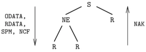
A “session” of the PGM protocol (a given data transfer from a source to a group of receivers) builds a tree: the source is the root of the tree, the receivers are the leaves, and the other network elements are intermediary nodes. This tree may change during the session by the dynamic join/leave of receivers. Figure 1 shows such a distribution tree and the direction (upstream or downstream) followed by the five basic packets of the protocol.
RDATA, SPM, NCF ODATA, NAK R R R NE S
Fig. 1.Distribution tree of the PGM with packets involved (S = source, NE = network element, R = receiver).
In the normal course of data transfer, a source multicasts sequenced data packets (ODATA) along a path of the distribution tree to the receivers. When a receiver detects missing data packets from the expected sequence, it unicasts repeatedly to the last network element of the path negative acknowledgments (NAKs) containing the sequence number of missing data. Network elements for-ward NAKs hop-by-hop to the source using the reverse path, and confirm each hop by multicasting a NAK confirmation (NCF) in response to the child from which the NAK was received. Receivers and network elements stop sending NAK at the reception of a corresponding NCF. Finally, the source itself receives and confirms the NAK by multicasting an NCF to the group. If the data missing is still in the memory, repairs (RDATA) may be provided by the source in response to the NAK. To avoid NAK implosion, PGM specifies procedures for NAK elimination within network elements in order to propagate just one copy of a given NAK along the reverse of the distribution path.
The basic data transfer operation is augmented by SPMs (Source Path Mes-sages) packets from a source, periodically interleaved with ODATA. SPMs have two functions. First, they carry routing informations used to maintain up-to-date PGM neighbor information and a fixed distribution tree. Second, they comple-ment the role of data packets when there is no more data to send by holding the state of the sender window. In this way, the receiver may detect data losses and send further NAKs.
Source functions. The source executes five functions: multicast of ODATA packets, multicast of SPMs, multicast of NCFs in response to any NAKs received, multicast of RDATA packets, and maintain (update and advance) of the transmit window. The transmit window plays an important role in the PGM operations. Any information produced by the application using PGM (upper level in the net-work layers) is put in the transmit window and split in several ODATA chunks, numbered circularly from 0 to 232− 1. This data is maintained in the window TXW SECStime units for further repairs and sent with a maximum transmit rate of TXW MAX RTE (bytes/seconds). The left edge of this window, TXW TRAIL, is de-fined as the sequence number of the oldest packet available for repairs. The right edge, TXW LEAD, is defined as the sequence number of the most recent data packet the source has transmitted. To provide information about the sender window, TXW TRAILedge is sent with O/RDATA and SPM packets and the TXW LEAD edge is included only in SPMs. If TXW TRAIL = TXW LEAD + 1, the window is considered empty. The maximum size of the window (TXW SIZE = TXW LEAD - TXW TRAIL + 1) should be less than 216− 1. The edge TXW LEAD is advanced when data is pro-duced by the application. The strategy of the source to advance the TXW TRAIL edge is not fixed in [SFC+
01].
Two types of SPMs are sent by the source: ambient SPMs are sent “at least sufficient” [SFC+
01] rate to maintain routing information; heartbeat SPMs are transmitted in absence of data at a decaying rate, in order to assist detection of lost data before the advance of the transmit window.
Receiver functions. The receiver executes five functions: receive O/RDATA within the transmit window and eliminate duplicates, unicast NAKs repeatedly until it receives a matching NCF if it detects a loss, suppress NAKs sending after the reception of the NCF, maintain a local receive window.
The receive window is determined entirely by the packets from the source, since it evolves according to the information received from the source (data packets and SPMs). For each session, the receiver maintains the buffer and the two edges of the window: RXW TRAIL is the sequence number of the oldest data packet available for repair from the source (known from data and SPMs) and RXW LEAD is the greatest sequence number of any received data packet within the transmit window.
Network element functions. Network element forwards ODATA without interven-tion. They play an important role in routing, NAKs reliability, and avoiding NAKs implosion. Indeed, they forward only the first copy of a NAK and discard NAKs for which they have repair data. They also forward RDATA only to the child which signaled by a NAKs the loss of the corresponding data.
3
Modeling PGM
It is easy to see that modeling the full PGM protocol is out of the scope of existing model-cheking tools, because we need to handle dynamic topology with
a lot of processes, dynamic routing, tens of counters and clocks per process, sequence numbers up to 232
− 1, etc.
In order to be able to look at the full reliability property, the first step consists of obtaining a “good” model. This model should be simple enough to be checked by the existing model-checking tools, but it has also to be realistic and to preserve the interesting behaviours for this property. To obtain such a model, we first analyze each dimension of complexity of PGM. For each dimension, we identify the abstractions that can be done and we specify those chosen for our model. This is the first step of our methodology.
3.1 Dimensions of complexity
First dimension considered is the topology. The general topology is a dynamic graph, but we argue that we can focus our attention on static topologies.
Indeed, we can abstract the dynamic graph of a session by a maximal static graph where all the nodes belonging to the group at a moment in the session are present. When a node joins the group at a moment t during a session, it behaves like a node which loses all the data sent between the beginning of the session and t. When a node leaves the group, it can be abstracted into a node which receives all the data in time, i.e., it is silent w.r.t. reliability of data transfer. In this case, we may ignore all of the mechanisms proposed for joining/leaving for nodes and for sending routing (distribution path) information.
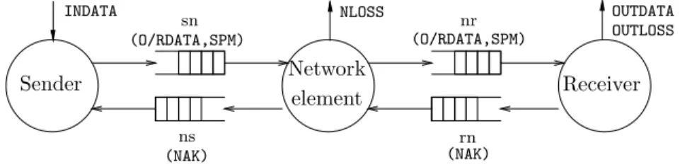
Moreover, the static distribution tree of a session may be abstracted into a linear topology. Indeed, if we consider that the loss rate does not depend on the number of receivers, adding more receivers to the tree does not change the advance of the transmit window. The loss of one data packet by several receivers may be abstracted by the loss detected in one receiver. More formal arguments in this direction are given in [EM02]. In conclusion, in order to study the full reliability property, we may consider linear topology with one source, one intermediate node, and one receiver, like in Figure 2.
(O/RDATA,SPM) Sender Receiver sn ns nr rn INDATA OUTDATA OUTLOSS NLOSS (O/RDATA,SPM) (NAK) (NAK) Network element
Fig. 2.Abstract model considered for topology and communication medium.
Second dimension considered is the policy of loss for packets. In the general case, any number of any kind of packets could be loss. We can reduce the huge non determinism of such behaviour by noting that NAK, NCF, and SPM packets
are small packets (they include one or two sequence numbers), for which the probability of loss using an IP network is small. Moreover, the loss of NAK and NCFpackets is dealt by special mechanisms executed locally (for each link). Then, we may consider that the transmission of control packets is reliable. For data packets, we consider that at most MAX NB LOSS ODATA packets are lost, where MAX NB LOSSis a parameter of the model. The transmission of RDATA packets is abstracted to be reliable, as proposed in [SFC+01].
The third dimension considered is the communication network. Since PGM is designed to work on IP, the model for communication is unbounded, unordered, unreliable channels with no maximal transmission delay. However, the protocol uses SPMsto carry routing informations in order to maintain a fixed distribution tree between sender and receivers. This allows us to abstract communication media to FIFO queues. The real-time feature of the protocol and the small sizes of PGM packets suggest us to put bounds on the size and the delays of com-munication channels. In conclusion, our comcom-munication media are reliable FIFO queues with bounded sizes and fixed delays of transmission (see Figure 2). Such a communication primitive is present in our modeling language, If [BFG+
00]. Losses of packets are simulated within the network element.
The next dimension concerns the length of information to be transmitted during the session w.r.t. the size of the transmit window. To cover most of the mechanisms of the protocol, this length should be greater than two transmit windows, and a transmit window should contain at least three data packets. This abstraction is implicitly used in [BBP02] since they consider that the maximal number of ODATA packets sent is ten. In our model, this length is a parameter, called MAX NB DATA.
Another dimension is the shape of the traffic from the application. In [SFC+
01] is suggested that the source should implement a scheme for the traffic management and it should also bound the maximum rate of transmission. Moreover, a local absence of data should also be managed by sending heartbeat SPMs. A simple abstraction that avoids the heartbeat mechanisms (i.e., additional packets) and reduces the traffic shape is to consider a fixed rate of information generation. This rate is given by a parameter, DATA PERIOD, specifying the time units between the generation of two data packets. The application sends the data at this rate until the end of the transmission. When this end is reached, the source signals it by a “closing SPM” [Boy02] packet containing the status of the window, which signals the absence of data and replaces the heartbeat mechanism.
The protocol also provides a lot of mechanisms to ensure efficiency of trans-mission. These mechanisms (e.g., filtering of NAKs in network elements, back-off timeouts for NAKs, filtering of RDATA) are not relevant to the reliability property that we aim to test.
Other mechanisms are introduced in order to obtain some properties for the transmission, mainly the reliability of the NAKs and NCFs. We abstract these mechanisms and consider that there are no loss of NAKs, so no need for NCFs.
The last dimension of complexity concern the management of the transmit window. In [SFC+
01], no policy is fixed for the advance of the window and the sending of the ambient SPMs. In our model, we consider that the sender tries to keep in the window the maximum number of data packets in such a way that it can receive any time data from application, i.e. TXW SIZE packets are always kept. When the application finishes the transmission, the packets are dropped out from the window each DATA PERIOD time units. Concerning the sending of ambient SPMs, we choose to send an ambient SPM for every DATA PER SPM data packets generated by the application, with DATA PER SPM a parameter of the protocol.
3.2 Abstract model considered
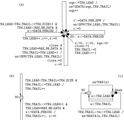
The second step consists of applying the abstractions described above in order to obtain a formal model of the PGM protocol. The models obtained for the PGM source, receiver, and network element are given respectively on Figures 3, 5, and 4. We explain in this section the resulting model.
We use If [BFG+00], which underlying model is a network of finite state, timed automata communicating by channels of different policies, rendez-vous, and shared variables. The finite types that can be used are boolean, bounded integer, user defined enumerated type, record and finite array of finite types. In If, states can be decorated with invariants for time elapsing. By default, the invariant is true. Unstable states are states where the time cannot pass (represented by a vertex with an U inside). Transitions are guarded by boolean expressions on finite variables, zones on clocks, and inputs from communication channels (notation c?s(x,y) for input from channel c of the signal s with data assigned to variables x and y). A special guard is the eager guard (represented by a transition with a black point at the source vertex) which means that the transition must be taken as soon as possible w.r.t. the synchronization with other transitions. If the guard is true, some actions can be executed before the control goes in the target state. The actions belong to reset clocks, assignment of finite variables, and output of messages on channels (notation c!s(x,y) for output on channel c of the signal s with data x and y). In order to obtain easy to read automata, the automaton of each component is split in several parts, each part has like source a shared state and implements a specific function (see Section 2) of the component.
The source inputs data from the upper level (increments TXW LEAD) each DATA PERIOD time units until the limit of MAX NB DATA is reached (Figure 3, Part (a)). Interleaved with this activity, the source sends ODATA packets in the transmit window as soon as (eager transition) the data is available. For every2 DATA PER SPM data packets generated by the application, the source sends an ambient SPM. When the MAX NB DATA limit is reached and all the data have been
2
Although the guard for this transition is c>=DATA PER SPM, the transition is eager, so it will be taken immediately when the value DATA PER SPM is reached.
(a) sn!SPM(TXW LEAD,TXW TRAIL) S0: x<=DATA PERIOD x:=0, c:=0, sqn:=0 close:=1 TXW TRAIL:=0 TXW LEAD:=-1 c:=0 close & c:=0 close:=0 TXW TRAIL=TXW LEAD+1 / TXW LEAD=MAX NB DATA &
x>=DATA PERIOD / TXW LEAD<MAX NB DATA &
sqn<=TXW LEAD /
(b)
TXW LEAD-TXW TRAIL=TXW SIZE & TXW TRAIL<=TXW LEAD / TXW TRAIL++
TXW TRAIL<=TXW LEAD+1 & TXW LEAD=MAX NB DATA & x>=DATA PERIOD / TXW TRAIL++, x:=0 S0
sn!SPM(TXW LEAD,TXW TRAIL) TXW LEAD-TXW TRAIL<=TXW SIZE+1 &
c>=DATA PER SPM / TXW LEAD++,c++,x:=0 sqn++ sn!ODATA(sqn,TXW TRAIL) TXW TRAIL<=n<=TXW LEAD / n>TXW LEAD n<TXW TRAIL Snak sn!RDATA(n,TXW TRAIL) U ns?NAK(n) (c) S0
Fig. 3.Model for the PGM source: (a) sending ODATA and SPM, (b) window advance, (c) dealing with NAK and RDATA.
i<RS LEN & RS[i]!=seq / Nnak Nspm nr!SPM(lead,trail),i:=0 sn?SPM(lead,trail) / (d) i=RS LEN RS[RS LEN++]:=seq ns!NAK(seq) i=RS LEN / i<RS LEN & RS[i]=seq
rn?NAK(seq) / i:=0 (c)
RS[i]:=RS[--RS LEN] nr!RDATA(seq,trail) i<RS LEN & RS[i]=seq /
i=RS LEN
i<RS LEN & Nodata
i<RS LEN & RS[i]!=seq / i++ Nrdata i++ i++ RS[i]:=RS[--RS LEN] RS[i]<trail / i<RS LEN & N0 N0 N0 N0 nloss:=0 RS LEN:=0 (b) (a) RS[i]>=trail / sn?RDATA(seq,trail) / i:=0 U U U U nloss++ env!NLOSS(seq) nloss<MAX NB LOSS / sn?ODATA(seq,trail) nr!ODATA(seq,trail)
Fig. 4.Model for the PGM network element: (a) dealing ODATA, (b) dealing RDATA, (c) dealing NAKs, (d) dealing SPMs.
RXW[0..RCV SIZE-1]:=0
(is xdata & sqn>RXW LEAD+1) Rupt
Rupt’ env!OUTDATA(RXW TRAIL)
RXW[RXW TRAIL%RCV SIZE] / RXW TRAIL<=RXW LEAD &
RXW[(++RXW LEAD)%RCV SIZE]:=0 R0 RXW LEAD:=-1 RXW TRAIL:=0 rn!NAK(RXW LEAD+1) RXW[sqn%RCV SIZE]:=1 RXW LEAD++
is xdata & sqn=RXW LEAD+1 / RXW[sqn%RCV SIZE]:=1 is xdata & sqn<=RXW LEAD / RXW[(RXW TRAIL++)%RCV SIZE]:=0
| (!is xdata & lead>RXW LEAD)
Rtrail
RXW[(RXW TRAIL++)%RCV SIZE]:=0
env!OUTLOSS(RXW TRAIL) !RXW[RXW TRAIL%RCV SIZE] /
RXW TRAIL<=RXW LEAD &
RXW LEAD++ env!OUTLOSS(RXW TRAIL)
RXW TRAIL>RXW LEAD / RXW TRAIL<=RXW LEAD & RXW[RXW TRAIL%RCV SIZE] / env!OUTDATA(RXW TRAIL) RXW TRAIL<trail Radt’ Radt (b) (a) Rtrail lead<=RXW LEAD U U U U U U
!is xdata & RXW TRAIL>=trail nr?ODATA(sqn,trail)/is xdata:=1 nr?RDATA(sqn,trail)/is xdata:=1 nr?SPM(lead,trail)/is xdata:=0
sent, a closing SPM packet is sent to inform the receiver about the absence of recovery. This solution has been proposed in [Boy02] to be able to give a cor-rect status about the data packets sent in the last transmit window in absence of heartbeat SPMs. Part (b) specifies the policy of window advance. Part (c) specifies the treatment of NAK.
The network element forwards ODATA packets (Figure 4, part (a)) or non deter-ministically losses data (signaled to the environment by the NLOSS signal). The sequence numbers of data to be recovered are stored in a vector RS of maximal size RS SIZE and of current size RS LEN. This vector is updated at the arrival of RDATA, NAK, and SPM packets (parts (b), (c), and (d) respectively). It is used to avoid duplication of NAKs.
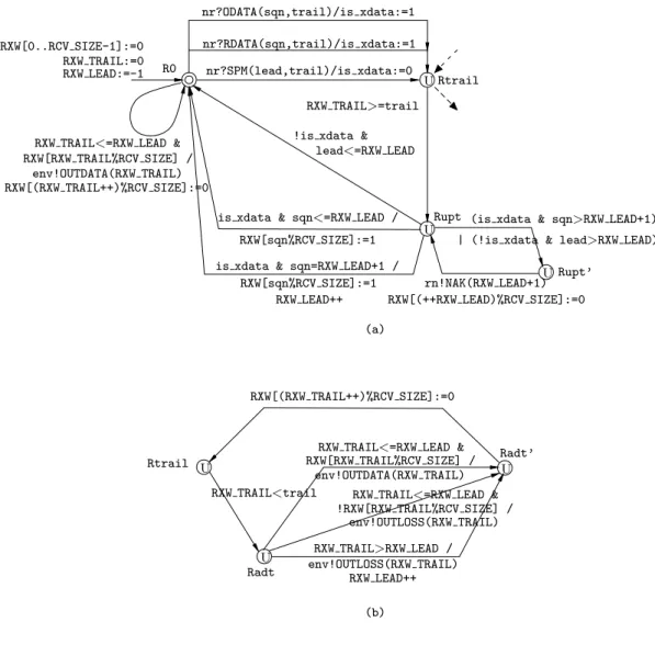
The receiver waits for any kind of packets (ODATA, RDATA, and SPM) and updates the receive window implemented by the array RXW (of maximal size RXW SIZE). This array is used as a circular buffer (sequence numbers taken modulo the size of the array) and it stores booleans saying if the corresponding data packet has been received or not. Initially, all the entries are false. Based on RXW array, when the transmit window advance (the trail received is greater than RXW TRAIL), the receiver sends either OUTDATA signal to the environment or it signals a loss (OUTLOSS signal).
The parameters of the model are summarized in Table 1. For each parameter we give either a value, if it has been fixed during experiments, or an interval of values otherwise. We discuss the choice of these value in Section 6.
Table 1.Summary of parameters. Size parameters
TXW SIZE Transmit window size 1–6
MAX NB LOSS Max. number of lost data at some point 0–5 MAX NB DATA Max. number of data the source can send 3–18 DATA PER SPM Nb. of data generated between two ambient SPM 1-3, ∞ RS SIZE Max. size of RS array MAX NB LOSS RXW SIZE Max. size of receiver window TXW SIZE SN SIZE, NS SIZE Max. size of sender-network element buffers 12, 4 NR SIZE, RN SIZE Max. size of network element-receiver buffers 12, 4
Time parameters
DATA PERIOD Period of data sending 2–10,15 TXW MAX RTE= 1/DATA PERIOD,
TXW SECS= (TXW SIZE − 1) × DATA PERIOD
SN DELAY, NS DELAY Max. delay for sender-network element buffers 2, 2 NR DELAY, RN DELAY Max. delay for network element-receiver buffers 2, 2
4
Constraint for recovering all losses
In the third step of our methodology, we analyze the sequence of events needed to obtain the target property. In our case, the sequence allowing to recover a loss ensures the full reliability. It involves four steps:
1. one or more ODATA packets are lost (by the node, in our model);
2. the receiver receives a packet (ODATA, RDATA, or SPM) signaling that a previous data packets have been lost;
3. the NAK signaling the loss is received by the source before the corresponding data have been dropped from the transmit window;
4. the corresponding RDATA is sent and received. These steps concern the following aspects of our model:
– the loss policy: in our model only MAX NB LOSS ODATA packets can be lost; – the transit delay of packets (i.e., round trip time, RTT): is computed from the
delays of communication buffers, RTT = SN DELAY + NR DELAY + RN DELAY + NS DELAY;
– the production rate of ODATA: given by DATA PERIOD;
– the rate of ambient SPM: given by DATA PER SPM and DATA PERIOD;
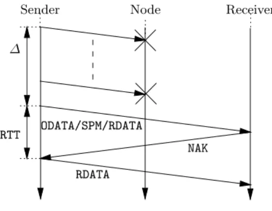
– the transmit window policy: fixed to maintain as long as possible data in the transmit window. NAK RDATA ODATA/SPM/RDATA ∆ RTT
Sender Node Receiver
Fig. 6.Pattern of loss recovering.
Let ∆ be the delay between the instant the first lost ODATA packet is sent and the instant that the first unlost packet is sent. The delay between the sending of the unlost packet and the reception of the matching NAK is the RTT, if we assume that a NAK is sent as soon as a loss is detected (it is the case in our model, but in a more realistic one, we should add a random back-off).
Then, the lost packets are recovered if ∆ + RTT is less than3
the lifetime of the data in the transmit window, i.e. DATA PERIOD × TXW SIZE in our model.
The value of ∆ depends on the kind of the first non-lost packet: ODATA, RDATA, or SPM, i.e., ∆ = min(∆ODATA, ∆RDATA, ∆SPM). We cannot give an upper bound of ∆RDATA. Indeed, it could be ∞ if no packet has been lost before. For ∆ODATA, if we consider that no more than MAX NB LOSS packets are lost, its maximum value is MAX NB LOSS × DATA PERIOD. This value is false for the last MAX NB LOSS packets since they can all be lost and not followed by any ODATA. For ∆SPM, the upper bound is (DATA PER SPM − 1) × DATA PERIOD (the -1 comes from the fact that the SPM is sent at the same time that the last ODATA of the DATA PER SPM set).
Then, we obtain the following property:
Property 1. If a data packet m does not belong to the last MAX NB LOSS packets, then m is always recovered if:
TXW SIZE− min (MAX NB LOSS, DATA PER SPM − 1) > RTT
DATA PERIOD (1)
5
Verification methodology and tools
The last step of our methodology is the verification of the constraint obtained using finite timed model-checking. It consists of the following actions:
1. We assign to parameters given in Table 1 relevant, concrete values (see Sec-tion 6).
2. Using these values, the parameterized model corresponding to the automata given on figures 3–5 is translated (by substitution) into a concrete model. 3. The concrete model is translated into a labeled transition system (LTS). 4. In order to check the model obtained, some basic, unparameterized
proper-ties like absence of deadlock, absence of overflows, etc. are checked on the LTS.
5. The parameterized property to be checked is also translated into a set of con-crete properties, one property per sequence numbers from 0 to MAX NB DATA (which is a parameter).
6. The concrete properties are checked on the LTS.
In order to instantiate parameterized implementation and properties to concrete ones, we use shell scripts calling sed commands. The translation from the If concrete implementation into the LTS is done using the generator tool of the If toolbox. The LTS model is generated into the Bcg [FGK+96] format. The temporal logic properties have been written using the regular alternation-free µ-calculus [Koz83,EL86] and checked using the evaluator tool [MS00] of the Cadp [FGK+96] toolbox. The tools used provide good performances: the time
3
The inequality is strict because of the possible interleaving of actions dropping the data from the window and sending RDATA.
and memory spent for generating and checking the models are reasonable for the values of parameters reported here4
. For example, the full series of experiments (≈ three hundred cases) take 4 hours on a PC at 1GHz and 1Go of RAM.
6
Experiments
6.1 Choosing relevant values for parameters
In searching relevant values for parameters, we follow three criteria:
C1: Cover all cases for both satisfaction values of Equation 1. This leads to a case analysis of Equation 1. When it is false, we may have two cases:
C1.1: TXW SIZE− min (MAX NB LOSS, DATA PER SPM − 1) ≤ 0
C1.2:0 < TXW SIZE − min (MAX NB LOSS, DATA PER SPM − 1) ≤ RTT/DATA PERIOD which implies RTT > DATA PERIOD
When Equation 1 is true, we may have also two cases:
C1.3: TXW SIZE− min (MAX NB LOSS, DATA PER SPM − 1) > RTT/DATA PERIOD ≥ 1 C1.4: TXW SIZE− min (MAX NB LOSS, DATA PER SPM − 1) ≥ 1 > RTT/DATA PERIOD C2: Choose values preserving the ratio between the real life values of
parame-ters. This criterion reduces the number of experiments selected with criterion C1. Indeed, we observe the following relation between the parameters: C2.1: The maximal number of losses MAX NB LOSS could be viewed like a
fraction 1/p of the maximal number of data sent MAX NB DATA. Then, MAX NB DATAmay be considered like a multiple n of the transmit window size, TXW SIZE. If we suppose that the network has a low rate of losses (e.g., p = 20), the value of n/p may vary, for example, between 0.05 when the number of data is small (e.g., n = 1) and 100 when the number of data is great (n ≈ 103
).
C2.2: The rate DATA PER SPM may belong to two classes of values. If DATA PER SPMis greater than MAX NB LOSS, it can be approximated to ∞ since the recover will not be done with SPMs packets. The second class of values is defined by the ratio between TXW SIZE and DATA PER SPM. A great ration (a lot of SPMs sent by transmit window) implies an overload of the network but ensures quick data recovery. Then, we have to test values greater and less than 1 for this ration.
C2.2: In real life, the RTT may vary considerably depending on the physical network. If the network is real-time oriented, the values taken by RTT may vary between 400ms to 40ms (ATM networks). For DATA PERIOD, the value given as example in [SFC+01] is ≈ 60ms. So, the interesting cases will concern values of RTT/DATA PERIOD ≥ 1 or closer to 1 (video applications usually run faster than the network).
C3: Choose values allowing to generate the LTSs. For example, we abstract the real values of TXW SIZE to values between 1–5. We do the same with RTT and DATA PERIOD values.
4
However, for values outside the set taken here, we obtain in some cases state explo-sion.
6.2 Properties checked
On the LTS generated from the model we checked properties like deadlock free-dom, absence of overflows for FIFOs, and a lost data packet is either signaled as lost or recovered. We used these properties only to check the correctness of our abstract model.
The temporal logic formulae φ used to prove Property 1 is: “ODATA packet number SQN is sometimes signaled as lost”. In the regular free µ-calculus, this formula is:
<true*.’.*sn_in,ODATA,{_SQN_},.*’.true*.’.*OUTLOSS,{_SQN_}.*’> true which means that it is possible to have a sequence of transitions having an input of ODATA with number SQN on queue sn (sub-string sn_in,ODATA,{_SQN_}) and then this packet is signaled as lost (sub-string OUTLOSS,{_SQN_}). The property is parameterized by the SQN number which belongs to 0..MAX NB DATA.
If the result of model-checking φ is false, then the packet is never signaled as lost (i.e. it is either no lost or always recovered).
6.3 Results and discussion
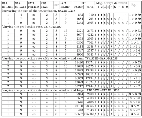
The results for a part of experiments done are presented on Tables 2–4. The experiments are looking to the truth value of checking φ while varying each parameter involved in the Equation 1. We report value b ∈ {t, f} in the columns corresponding to a given sequence number if the result of checking φ for this sequence number is ¬b. The results in italic correspond to (unrelevant) cases when the sequence number does not satisfy the hypothesis of Property 1 or Equation 1 is not satisfied (see the last column of tables).
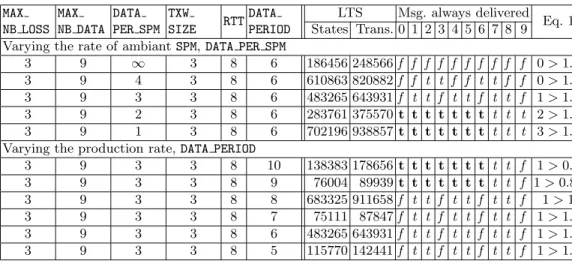
The tables 2 and 3 report about the recover of losses based on ∆ODATA (assuming ∆SPM = ∞). Table 4 reports about the impact of ambient SPMs. In all these tables we limit our report to experiments with an RTT value fixed to 8. Instead, we vary the value of DATA PERIOD in order to cover all the cases defined at the beginning of this section. The last paragraph below reports on the consequences of varying the RTT value.
Recovery based on ODATA This case corresponds to DATA PER SPM > MAX NB LOSS. The eight series of experiments done vary the three remaining parameters (MAX NB LOSS, TXW SIZE, and DATA PERIOD). Note that in all config-urations tested in Tables 2 and 3, the MAX NB LOSS last packets may be defini-tively lost. So, the hypothesis of Property 1 is checked to be important. Another interesting result is the check of the necessity of Equation 1 since when it is false, all the packets (with numbers satisfying or not the hypothesis of Property 1) can be lost.
Recovery based on SPM To test this case, we consider only configurations where DATA PER SPM< MAX NB LOSS, except the first line of Table 4 which is used to show the difference between the recovering based on ODATA and on SPM. Indeed,
Table 2.Effect of the production rate DATA PERIOD on the loss recovery. MAX NB LOSS MAX NB DATA DATA PER SPM TXW SIZE RTT DATA PERIOD LTS Msg. always delivered Eq. 1 States Trans. 0 1 2 3 4 5 6 7 8 9 Increasing the size of the transmission, MAX NB DATA
1 4 ∞ 2 8 9 853 910 t t t t f − − − − − 1 > 0.89 1 7 ∞ 2 8 9 1684 1795 t t t t t t t f − − 1 > 0.89 1 9 ∞ 2 8 9 2353 2505 t t t t t t t t t f 1 > 0.89 Varying the production rate, DATA PERIOD
1 9 ∞ 2 8 15 2321 2473 t t t t t t t t t f 1 > 0.53 1 9 ∞ 2 8 10 3607 4222 t t t t t t t t t f 1 > 0.8 1 9 ∞ 2 8 9 2353 2505 t t t t t t t t t f 1 > 0.89 1 9 ∞ 2 8 8 6390 7601 f f f f f f f f f f 1 > 1 1 9 ∞ 2 8 7 2113 2238 f f f f f f f f f f 1 > 1.1 1 9 ∞ 2 8 5 2347 2557 f f f f f f f f f f 1 > 1.6 1 9 ∞ 2 8 3 4960 5941 f f f f f f f f f f 1 > 2.7 Varying the production rate with wider window and same TXW SIZE−MAX NB LOSS
2 9 ∞ 3 8 15 11420 13074 t t t t t t t t f f 1 > 0.53 2 9 ∞ 3 8 10 19649 24575 t t t t t t t t f f 1 > 0.8 2 9 ∞ 3 8 9 11829 13498 t t t t t t t t f f 1 > 0.89 2 9 ∞ 3 8 8 60393 78011 f f f f f f f f f f 1 > 1 2 9 ∞ 3 8 7 10853 12194 f f f f f f f f f f 1 > 1.1 2 9 ∞ 3 8 5 17623 21324 f f f f f f f f f f 1 > 1.6 2 9 ∞ 3 8 3 33717 42744 f f f f f f f f f f 1 > 2.7 Varying the production rate with wider window and bigger TXW SIZE−MAX NB LOSS
1 9 ∞ 4 8 15 2344 2489 t t t t t t t t t f 3 > 0.53 1 9 ∞ 4 8 10 3532 4088 t t t t t t t t t f 3 > 0.8 1 9 ∞ 4 8 5 3546 4106 t t t t t t t t t f 3 > 1.6 1 9 ∞ 4 8 4 21180 28065 t t t t t t t t t f 3 > 2 1 9 ∞ 4 8 3 6443 7848 t t t t t t t t t f 3 > 2.7 1 9 ∞ 4 8 2 155587 225502 f f f f f f f f f f 3 > 4
Table 3.Effect of the number of losses MAX NB LOSS and of the window size TXW SIZE on the loss recovery.
MAX NB LOSS MAX NB DATA DATA PER SPM TXW SIZE RTT DATA PERIOD LTS Msg. always delivered Eq. 1 States Trans. 0 1 2 3 4 5 6 7 8 9
Varying the window size, TXW SIZE
1 9 ∞ 4 8 9 2376 2521 t t t t t t t t t f 3 > 0.89 1 9 ∞ 3 8 9 2366 2515 t t t t t t t t t f 2 > 0.89 1 9 ∞ 2 8 9 2353 2505 t t t t t t t t t f 1 > 0.89 1 9 ∞ 1 8 9 2098 2225 f f f f f f f f f f 0 > 0.89 Varying the window size and faster source, i.e. less DATA PERIOD
1 9 ∞ 4 8 8 6088 7203 t t t t t t t t t f 3 > 1 1 9 ∞ 3 8 8 6440 7641 t t t t t t t t t f 2 > 1 1 9 ∞ 2 8 8 6390 7601 f f f f f f f f f f 1 > 1 1 9 ∞ 1 8 8 4053 4929 f f f f f f f f f f 0 > 1 Varying the window size and more losses
2 9 ∞ 5 8 9 11915 13566 t t t t t t t t f f 3 > 0.89 2 9 ∞ 4 8 9 11878 13540 t t t t t t t t f f 2 > 0.89 2 9 ∞ 3 8 9 11829 13498 t t t t t t t t f f 1 > 0.89 2 9 ∞ 2 8 9 10597 11934 f f f f f f f f f f 0 > 0.89 2 9 ∞ 1 8 9 7992 8536 f f f f f f f f f f −1 > 0.89 Varying the number of losses
0 9 ∞ 5 8 9 248 253 t t t t t t t t t t 5 > 0.89 1 9 ∞ 5 8 9 2383 2523 t t t t t t t t t f 4 > 0.89 2 9 ∞ 5 8 9 11915 13566 t t t t t t t t f f 3 > 0.89 3 9 ∞ 5 8 9 46368 55966 t t t t t t t f f f 2 > 0.89 4 9 ∞ 5 8 9 136148 170412 t t t t t t f f f f 1 > 0.89 5 9 ∞ 5 8 9 307266 391888 f f f f f f f f f f 0 > 0.89
Table 4.Effect of the ambient rate DATA PER SPM on the loss recovery. MAX NB LOSS MAX NB DATA DATA PER SPM TXW SIZE RTT DATA PERIOD LTS Msg. always delivered Eq. 1 States Trans. 0 1 2 3 4 5 6 7 8 9 Varying the rate of ambiant SPM, DATA PER SPM
3 9 ∞ 3 8 6 186456 248566 f f f f f f f f f f 0 > 1.3 3 9 4 3 8 6 610863 820882 f f t t f f t t f f 0 > 1.3 3 9 3 3 8 6 483265 643931 f t t f t t f t t f 1 > 1.3 3 9 2 3 8 6 283761 375570 t t t t t t t t t t 2 > 1.3 3 9 1 3 8 6 702196 938857 t t t t t t t t t t 3 > 1.3 Varying the production rate, DATA PERIOD
3 9 3 3 8 10 138383 178656 t t t t t t t t t f 1 > 0.8 3 9 3 3 8 9 76004 89939 t t t t t t t t t f 1 > 0.89 3 9 3 3 8 8 683325 911658 f t t f t t f t t f 1 > 1 3 9 3 3 8 7 75111 87847 f t t f t t f t t f 1 > 1.1 3 9 3 3 8 6 483265 643931 f t t f t t f t t f 1 > 1.3 3 9 3 3 8 5 115770 142441 f t t f t t f t t f 1 > 1.6
in the configuration corresponding to the first line, all packets are lost, but in the next configurations, all packets satisfying the hypothesis are recovered. An interesting point is that, even if the Equation 1 is not satisfied, some packets are always recovered (two per DATA PER SPM period). In fact, some packets sent before an SPM can always be recovered because the sum ∆SPM + RTT is small enough to recover before the window advance.
In both cases, when DATA PERIOD is increased, the number of packets lost increases.
Considerations on sizes of LTSs In some series of experiments, the size of the state space increases globally, but not locally. It is particularly visible on the second, third, and forth series of Table 2. This global increase seems “normal”: there are more packets in the system when DATA PERIOD increases so the system is more “complex”.
Nevertheless, there are some local decreases: in the second series of Table 2, when DATA PERIOD decreases from 10 to 9 or from 8 to 7, etc., and in the second series of Table 4 when DATA PERIOD decreases from 10 to 9 and from 8 to 7. The explanation we found to this phenomenon involves the RTT and DATA PERIOD. Indeed, when RTT and DATA PERIOD are coprime, there are less events to inter-leave than when they have a common divisor. So the sizes of LTSs are smaller in the first case than in the second. To check this explanation, we also did the experiments of in Table 2 with different values of RTT (more details presented in [Boy02]).
7
Conclusion
The verification and synthesis problems for parameterized system are difficult problems when the parameters are related by non-linear relations. In this paper we propose a methodology using finite and real-time model-checking to deal with the synthesis problem on such systems. Of course, the problem of synthesis is not completely managed. We obtain a relation by carefully modeling and analyzing the protocol.
Such a work gives some ideas about how the existing finite verification tools can be used to deal with parameterized verification. At the present time, the use of Unix shell scripts seems to be unavoidable because there are no means to easily instantiate parameters in models and properties. It would be useful to have specification languages and verification scripts allowing to specify parameterized models and properties and then to instantiate these specifications with actual values in a functional style.
Another contribution is design of a (static but almost complete) formal model for the PGM protocol and the synthesis of the constraint between its parameters. The modeling process allows us to signal some lacks in the reference specification. Finally, by doing the present work, we won the experience for obtaining sim-pler models for PGM such that they can be managed by the existing tools for infinite state systems. Indeed, the abstract model considered here is too com-plex for tools doing parameterized model-checking, e.g. TReX [BCAS01]. The
sources of complexity are the great number of infinite domain variables (since finite integer variables are now considered as counters), and the non-linear re-lation between integer parameters. First experiments with TReX lead to mem-ory explosion due to the size of symbolic representation used for parameterized configurations for clocks and counters. By looking at these representations, we obtain some hints about how to reduce their size. For example, the use of live analysis for counter variables may be useful due to the lack of communication by shared variables.
References
[AAB00] A. Annichini, E. Asarin, and A. Bouajjani. Symbolic techniques for para-metric reasoning about counter and clock systems. In E.A. Emerson and A.P. Sistla, editors, Proceedings of the 12th CAV, volume 1855 of LNCS, pages 419–434. Springer Verlag, July 2000.
[AHV93] R. Alur, T.A. Henzinger, and M.Y. Vardi. Parametric real-time reasoning. In ACM Symposium on Theory of Computing, pages 592–601, 1993. [BBP02] B. B´erard, P. Bouyer, and A. Petit. Analysing the pgm protocol with
up-paal. In P. Pettersson and W. Yi, editors, Proceedings of the 2nd Workshop RT-TOOLS, Copenhagen (Denmark), August 2002.
[BCALS01] A. Bouajjani, A. Collomb-Annichini, Y. Lackneck, and M. Sighireanu. Analysing fair parametric extended automata analysis. In Proceedings of SAS’01, LNCS. Springer Verlag, July 2001.
[BCAS01] A. Bouajjani, A. Collomb-Annichini, and M. Sighireanu. Trex: A tool for reachability analysis of complex systems. In Proceedings of CAV’01, LNCS. Springer Verlag, 2001.
[BFG+00] M. Bozga, J.-C. Fernandez, L. Girvu, S. Graf, J.-P. Krimm, and L. Mounier.
If: A validation environment for times asynchronous systems. In E.A. Emer-son and A.P. Sistla, editors, Proceedings of the 12th CAV, volume 1855 of LNCS, pages 543–547. Springer Verlag, July 2000.
[BL02] B. Boigelot and L. Latour. ADVANCE Project Deliverable Report, chapter Verifying PGM with infinitely many packets. LIAFA, 2002.
[Boi98] B. Boigelot. Symbolic Methods for Exploring Infinite State Spaces. PhD thesis, University of Li`ege, 1998.
[Boy02] M. Boyer. On modeling and verifying the pgm protocol. Technical report, LIAFA, 2002.
[Bul98] T. Bultan. Automated symbolic analysis of reactive systems. PhD thesis, University of Maryland, 1998.
[EL86] E. A. Emerson and C-L. Lei. Efficient model checking in fragments of the propositional mu-calculus. In Proceedings of the 1st LICS, pages 267–278, 1986.
[EM02] J. Esparza and M. Maidl. ADVANCE Project Deliverable Report, chapter Verifying PGM with infinitely many topologies. LIAFA, 2002.
[FGK+
96] J.-C. Fernandez, H. Garavel, A. Kerbrat, R. Mateescu, L. Mounier, and M. Sighireanu. Cadp (cæsar/aldebaran development package): A protocol validation and verification toolbox. In R. Alur and T.A. Henzinger, editors, Proceedings of the 8th CAV, volume 1102 of LNCS, pages 437–440. Springer Verlag, August 1996.
[HRSV01] T. Hune, J. Romijn, M. Stoelinga, and F. Vaandrager. Linear parametric model checking of timed automata. In Proceedings of TACAS’01, 2001. [Koz83] D. Kozen. Results on the propositional µ-calculus. Theoretical Computer
Science, 27:333–354, 1983.
[MS00] R. Mateescu and M. Sighireanu. Efficient on-the-fly model-checking for regular alternation-free mu-calculus. In Proceedings of the 5th International Workshop on Formal Methods for Industrial Critical Systems FMICS’2000 (Berlin, Germany), April 2000.
[PL00] P. Pettersson and K.G. Larsen. Uppaal2k. Bulletin of the European As-sociation for Theoretical Computer Science, 70:40–44, February 2000. [SFC+
01] Tony Speakman, Dino Farinacci, Jon Crowcroft, Jim Gemmell, Steven Lin, Dan Leshchiner, Michael Luby, Alex Tweedly, Nidhi Bhaskar, Richard Ed-monstone, Todd Montgomery, Luigi Rizzo, Rajitha Sumanasekera, and Lorenzo Vicisano. PGM reliable transport protocol specification. RFC 3208, IETF, Decembre 2001. 111 pages.