Algorithmic and Computational Advances for
Fast Power System Dynamic Simulations
Petros Aristidou
Thierry Van Cutsem
Abstract—In this paper, some algorithmic and computational
advances are presented for power system dynamic simulations. The heart is a Schur-complement-based solution algorithm, stemming from domain decomposition methods, applied to the differential-algebraic equation model. This algorithm is then accelerated computationally, by employing parallel computing techniques, and numerically, by exploiting time-scale decomposi-tion and localizadecomposi-tion. Models of a real medium-scale system and a realistic large-scale test system are used for the performance evaluation of the proposed methods.
Index Terms—dynamic security assessment, differential-algebraic equations, time simulation, Schur-complement, parallel processing, Newton method, localization
I. INTRODUCTION
Over the last decades, dynamic simulations have become indispensable in the planning, design, operation and security assessment of power systems. They find application in power system operator training, analyzing large sets of scenarios, assessing the dynamic security of the network in real-time or scheduling the day-ahead operation.
In this type of simulations, complex electric components (like generators, motors, loads, wind turbines, etc.) are rep-resented by systems of stiff, non-linear Differential and Al-gebraic Equations (DAEs) [1]. Conversely, the network con-necting the equipment together is represented by a system of linear algebraic equations. Thus, a large interconnected system may involve hundreds of thousands of such equations whose dynamics span over very different time scales and, in addition, undergo many discrete transitions imposed by limiters, switching devices, etc.
When an application concerns the security of the system, the speed of simulation is a critical factor [2]. In the remaining, non-critical, applications the speed of simulation is desired as it increases productivity and minimizes costs. This is the main reason why control center applications often resort to faster, static simulations. However, with the operation of non-expandable grids closer to their stability limits, unplanned generation patterns stemming from renewable energy sources and active demand response schemes directed by electricity markets, it is likely that system security will be more and more guaranteed by emergency controls. In this context, checking the sequence of events that take place after the initiating disturbance is crucial; a task for which the static calculation
Petros Aristidou is with the Dept. of Elec. Eng. and Comp. Science, University of Liège, Liège, Belgium, e-mail: [email protected]
Thierry Van Cutsem is with the Fund for Scientific Research (FNRS) at Dept. of Elec. Eng. and Comp. Science, University of Liège, Liège, Belgium, e-mail: [email protected]
of the operating point in a guessed final configuration is inappropriate.
In this paper, a Schur-complement-based algorithm is first presented, which accurately solves the DAEs of the power system model over a discretized time horizon. It utilizes a simple partitioning to perform the solution in a decomposed manner, thus allowing the independent treatment of individual power system components. Then, the proposed algorithm is accelerated computationally and numerically to provide faster dynamic simulations.
First, it will be shown how the proposed domain decompo-sition allows for the application of modern parallel processing techniques, thus exploiting the computational power available in many inexpensive, shared-memory parallel computers. Sec-ond, it will be shown how the different time-scales of phe-nomena under study can be exploited by a stiff-decay solver to accelerate the algorithm while still monitoring discrete events triggered by the initial disturbance. Finally, it will be shown how the localized response to some disturbances can be used to further reduce the simulation time by performing less computations on elements with “lower dynamic activity”. By combining these three acceleration techniques (acc. tech.), fast and accurate dynamic simulations can be performed.
This is a paper accompanying a Panel presentation at the 2014 IEEE PES General Meeting. The work presented here unifies and extends the previous works [3], [4], [5] and [6]. New simulation results are provided and the benefit of combining the three acceleration techniques is investigated. The paper is organized as follows. In Section II the Schur-complement-based solution algorithm is presented. In Section III, the three proposed acc. tech. are summarized. Simulation results are reported in Section IV and followed by closing remarks in Section V.
II. SCHUR-COMPLEMENT-BASEDALGORITHM
Let the power system be decomposed into the network and a number of components, as sketched in Fig. 1. For reasons of simplicity, all components connected to the network, pro-ducing or consuming power, are called injectors.
On the one hand, each injector i is described by a system of non-linear DAEs [1]:
Γix˙i= Φi(xi, V ) (1)
where V is the vector of rectangular components of bus voltages, xi is the state vector containing differential and
Network
M M M M InjectorsFigure 1. Decomposed Network
matrix with: (Γi)ℓℓ=
{
0 if the ℓ-th equation is algebraic 1 if the ℓ-th equation is differential. On the other hand, the linear algebraic network equations take on the form:
0 = DV − I = DV −
n
∑
i=1
Cixi≜ g(x, V ) (2)
where D includes the real and imaginary parts of the bus admittance matrix, I is the vector of rectangular components of the bus currents, and Ci is a trivial matrix with zeros
and ones whose purpose is to extract the injector current components from xi.
For the purpose of numerical simulation, the injector DAE systems (1) are algebraized using a differentiation formula, such as Trapezoidal Rule or Backward Differentiation For-mulae (BDF), to get the corresponding non-linear algebraized systems:
0 = fi(xi, V ), i = 1, . . . , n. (3)
At each discrete time-step tn the non-linear algebraized
injector equations (3) are solved together with the network equations (2) using a Newton method to compute the vectors x(tn) and V (tn). At the k-th Newton iteration, the linearized
injector systems have to be solved simultaneously with the linear network equations (i = 1, . . . , n):
Ai∆xi+ Bi∆V =−fi(xki−1, V
k−1) (4)
D∆V− ∑ni=1Ci∆xi =−g(xk−1, Vk−1) (5)
The solution is computed using the decomposed and accel-erated Newton scheme detailed in [3]. In brief, the injector equations (4) are solved with respect to ∆xi, which is
intro-duced in (5) to obtain the following reintro-duced system: (D + n ∑ i=1 CiA−1i Bi)∆V =− g(xk−1, Vk−1) (6) − n ∑ i=1 CiA−1i fi(xki−1, V k−1)
This reduced system is solved to obtain the voltage correction ∆V which is backward substituted in (4) to get the state corrections ∆xi.
While this decomposition method is numerically equivalent to an integrated Newton scheme applied to equations (2) and (3), it provides access to the individual injector models and allows their separate treatment. This feature is exploited to accelerate the simulation procedure by parallelizing the independent calculations and employing localization.
III. ACCELERATIONTECHNIQUES
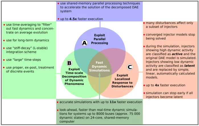
The presented Schur-complement-based algorithm opens the way for faster while accurate power system dynamic simulations. Namely, three acc. tech., summarized in Fig. 2, applied to that algorithm will be presented.
A. Parallel Computing
The parallel processing opportunities inherent to domain decomposition methods are exploited using shared-memory parallel programming techniques to take advantage of the computational resources available in multi-core computers. This is achieved by parallelizing the independent calculations relative to individual injectors.
Two steps of the presented algorithm are parallelized. First, the algebraization of the injector DAE systems (1) to get the corresponding non-linear algebraized systems (3), the linearization of the latter to calculate the individual Jacobian matrices, the factorization of the matrices and the calculation of the elimination factors CiA−1i Bi and CiA−1i fi. Second,
the solution of the linearized systems (4) to compute the state corrections ∆xi and the convergence check of the injector
DAE models. These two parallelized steps sum up for almost 80% of the total computing time.
B. Time-scale Decomposition
When considering long-term dynamic simulations (i.e. for long-term voltage stability), some fast components of the response may not be of interest and could be partially or totally omitted to provide faster simulations. This can be achieved either through the use of simplified models [7] or with a dedicated solver applying time-averaging [5].
While model simplification offers a big acceleration with respect to detailed simulation, some drawbacks exist. First, the separation of slow and fast components might not be possible for complex or black-box models. Furthermore, there is a need to maintain both detailed and simplified models. Finally, if both short and long-term evolutions are of interest, simplified and detailed simulations must be properly coupled [7].
At the same time, solvers using “stiff-decay” (L-stable) integration methods, such as BDF, with large enough time-steps can discard some fast dynamics. Such a solver, applied on a detailed model, can “filter” out the fast dynamics and concentrate on the average evolution of the system. The most significant advantage of this approach is that it processes the detailed, referenced model. Furthermore, this technique allows combining detailed simulation for short-term by limiting the time-step size, and time-averaged long-term by increasing it.
As power systems are described by hybrid models, an important consideration when increasing the time-step size is
Figure 2. Proposed Acceleration Techniques for Schur-complement-based Algorithm
the treatment of the discrete events. In the context of time-averaging an ex-post treatment of discrete events can be used as detailed in [5]. Summarizing the scheme used, at any time
t a time-step h is taken and the corresponding state vector x(t + h) is computed. Then, the system is checked for any violated discrete event conditions. If it is detected that a discrete event has occurred within the time-step, the equations (1) are changed accordingly and the step t→ t+h is repeated to compute a new state vector x(t + h). The algorithm uses the previously computed x(t + h) as initial vector to solve the perturbed equations (“warm-start”), thus significantly reducing the computational cost. This procedure is repeated, updating the state vector, until no more discrete conditions are violated or a maximum number of repetitions is reached. This yields the final state vector for the current step.
C. Localization
The concept of localization results from the observation that in a large power system a disturbance may affect only a small number of components. This fact is exploited in two ways.
First, it is used within one discretized time instant solution to stop computations of injectors whose DAE models have already been solved with the desired tolerance. That is, after one decomposed solution of (4) and (5), the convergence of each injector is checked individually. If the convergence criterion ( ∆xi
xi
< tol) is satisfied, then the specific injector is flagged as converged. For the remaining iterations of the current time instant, the injector is not solved, although its mismatch, computed with (3), is monitored to guarantee that
it remains converged. This technique decreases the compu-tational effort within one discretized time instant without affecting the accuracy of the solution [3].
Second, localization is exploited over several time steps by detecting, during the simulation, the injectors marginally participating to the system dynamics (latent) and replacing their dynamic models (1) with much simpler and faster to compute sensitivity-based models. At the same time, the full dynamic model is used if an injector exhibits significant dynamic activity (active). The sensitivity-based model used is derived from the linearized equations (4) when ignoring the internal dynamics, that is fi(xki−1, V
k−1)≃ 0, and solving
for the state variation ∆xi:
∆xi ≃ −A−1i Bi∆V
The corresponding current variation ∆Ii is given by:
∆Ii=−EiA−1i Bi∆V =−Gi∆V (7)
where Ei (similarly to Ci) is a trivial matrix with zeros and
ones whose purpose is to extract the injector current variations from ∆xi and Gi is a sensitivity matrix relating the current
with the voltage variation.
The technique employs simple and fast to compute metrics, originating from real-time digital signal processing, to classify each component into active or latent [6]. In brief, the vari-ability of each injector’s active and reactive powers (Pi, Qi)
is quantified by computing their standard deviations (Pstd−i,
Qstd−i) over a moving time-window. Standard deviations
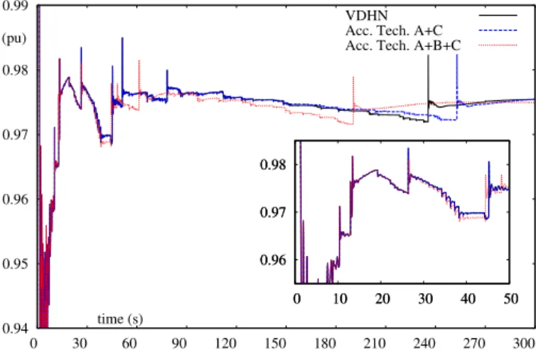
0.94 0.95 0.96 0.97 0.98 0.99 0 30 60 90 120 150 180 210 240 270 300 (pu) time (s) VDHN Acc. Tech. A+C Acc. Tech. A+B+C
0.96 0.97 0.98 0 10 20 30 40 50 0.96 0.97 0.98 0 10 20 30 40 50
Figure 3. 2204-bus System: Accuracy of Voltage Evolution
average. A small standard deviation indicates that the data points tend to be very close to the average.
Consequently, if both Pstd−iand Qstd−iare smaller than a
chosen tolerance (ϵL), the i-th injector is considered to exhibit
low dynamic activity and is declared latent. Thus, the full dynamic model (1) is replaced by the linear sensitivity-based (7). The tolerance value ϵL controls the trade-off between
acceleration and accuracy. In practice, a tolerance ϵL ≤ 0.5
(MW/MVAr) has been shown to provide significant speedup over several time-steps while maintaining high accuracy [6].
The average and standard deviations are computed using as efficient recursive formula [6], which is equivalent to observing the system response over a time-window.
Finally, the localization technique can be used to detect when the simulated system has reached a new steady-state equilibrium. That is, if all injectors in the system are declared latent at the same time, it is a good indication that the system has reached a new equilibrium state. Hence, the simulation can stop early without overlooking any dynamics.
IV. RESULTS
The Schur-complement-based algorithm with the acc. tech. sketched in Fig. 2 are implemented in RAMSES, developed at the University of Liège. RAMSES uses the OpenMP appli-cation programming interface for the parallelization. All the simulation results have been obtained with a 24-core AMD Opteron Interlagos desktop computer running Debian Linux.
The well-known, simultaneous Very DisHonest Newton (VDHN) algorithm applied on the original system (1), (2) is used for comparison [4]. In this scheme, the Jacobian matrix is updated and factorized only if the system hasn’t converged after three Newton iterations at any discrete time instant. This update strategy gives the best performance for the following test-cases. The VDHN simulations are performed with one-cycle time steps.
Concerning the localization parameters, an equivalent ob-servation time window of 20 s and a tolerance ϵL = 0.1
(MW/MVAr) were chosen in both test-systems, whenever localization is used. 1 3 5 7 9 11 13 15 1 2 4 6 8 10 12 14 16 18 20 22 24 Speedup # of cores
Acc. Tech. A+C Acc. Tech. A+B+C
Figure 4. 2204-bus System: Speedup A. 2204-bus System
This medium-scale model of a real system includes 2204 buses, 2919 branches and 135 power plants with a detailed rep-resentation of the synchronous machine, its excitation system, automatic voltage regulator, power system stabilizer, turbine and speed governor. The model also includes 976 dynamically modeled loads. The resulting DAE system has 11774 states. The disturbance consists of a bus bar fault lasting 7 cycles, that is cleared by opening two lines. Following, the system is simulated over an interval of 300 s. It evolves in the long term under the effect of 1076 Load Tap Changers (LTCs), 24 Automatic Shunt Compensation Switching (ASCS) devices as well as OvereXcitation Limiters (OXL).
Figure 3 shows the voltage at the faulted bus simulated by respectively the VDHN, the presented algorithm with acc. tech. A and C, and with all three techniques. Thus, for the first two simulations, a time step size of one cycle was used throughout the whole simulation; while, for the last, a time step of one cycle until t = 15 s (short term) and 0.1 s thereafter.
The short-term response (Fig. 3, zoom) is identical in all three curves. Due to the high dynamic activity observed during this period, the localization technique retains the injector DAE models. In the long-term, some small deviations are observed between the responses due to time-averaging and localization. The discrepancies are mainly due to the marginal activation of the ASCS devices. Their activation is identified correctly in all three simulations but some actions are shifted in time. However, the biggest voltage deviation between responses is in the order of 0.001 pu, which can be considered negligi-ble for most applications. Moreover, their final, steady-state, equilibrium is the same.
Figure 4 shows the speedup obtained with acc. tech. A and C and with all three techniques. It can be seen that the pro-posed techniques perform, respectively, three and seven times faster than the VDHN even in sequential execution. When using parallel computing, the proposed techniques simulate the disturbance in 48 s (resp. 16 s) compared to 252 s needed by VDHN, achieving a speedup of 5.2 (resp. 15.3) times. Parallelization drives the simulation speedup in the short-term, when high dynamic activity is observed, as most injectors are in active mode and their solutions more computationally intensive. When moving to long term, techniques B and C offer more acceleration by decreasing the computational burden.
0 30 60 90 120 150 180 210 240 270 300 0 30 60 90 120 150 180 210 240 270 300 Wall time (s) Simulation time (s) Real-time VDHN (1-core) Acc. Tech. A+C (1-core) Acc. Tech. A+C (6-cores) Acc. Tech. A+C (12-cores)
0 1 2 3 4 5 0 1 2 3 4 5
Figure 5. 2204-bus System: Real-time Performance
Figure 5 shows the real-time performance of the algorithm with two of the techniques. When the wall time curve is above the real-time line, then the simulation is lagging; otherwise, the simulation is faster than real-time and can be used for more demanding applications, like look-ahead simulations, training simulators or hardware/software in the loop [2]. On this power system, the algorithm performs faster than real-time when executed on six or more cores. Using all 24-cores, the algorithm can simulate in real-time power system models of up to 8000 buses and approximately 75000 dynamic states.
B. 15226-bus System
This large-scale model, representative of the continental European main transmission grid [3], includes 15226 buses, 21765 branches and 3483 power plants with a detailed repre-sentation of each synchronous machine, its excitation system, automatic voltage regulator, power system stabilizer, turbine and speed governor. The model also includes 7211 dynami-cally modeled loads. The resulting DAE system has 146239 differential-algebraic states. The disturbance consists of a bus bar fault, lasting five cycles, that is cleared by opening two double-circuit lines. The system is simulated over a period of 240 s. The system evolves in the long term under the effect of LTCs as well as OXLs. A time-step size of one cycle was chosen for the first 15 s (short term), followed by 2.5 cycles for the remaining (long term).
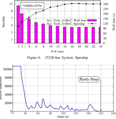
Figure 6 shows the speedup obtained with all three tech-niques. The disturbance is simulated in less than 100 s, more than 11 times faster than VDHN, when executed on 16 or more cores.
Figure 7 shows the activity of the injectors based on the above mentioned localization criterion. It can be seen that a large percentage of the injectors does not show “high dynamic activity”, especially in the long term. In the particular simulation, at around t = 210 s all injectors are declared latent, indicating that the system has reached a new equilibrium and simulation can be stopped.
V. CONCLUSION
In this paper, some algorithmic and computational advances have been presented to accelerate power system dynamic
1 3 5 7 9 11 1 2 4 6 8 10 12 14 16 18 20 22 24 0 30 60 90 120 150 180 210 240 Speedup Wall time (s) # of cores VDHN=1079s
Acc. Tech. A+B+C: Wall time Acc. Tech. A+B+C: Speedup
Figure 6. 15226-bus System: Speedup
0 30 60 90 120 150 180 210 240 time (s) 0 2000 4000 6000 8000 10000 A ct iv e In je ct o rs Early Stop
Figure 7. 15226-bus System: Active Injectors
simulations. Using the Schur-complement-based solution al-gorithm, three acc. tech. have been presented.
First, the solution is accelerated computationally with the use of shared-memory parallel computing techniques. Second, time-averaging is employed (with the use of a “stiff-decay” integration scheme, large time steps and ex-post discrete event handling) to “filter” out the fast dynamics and concentrate on the average evolution of the system for long-term simulations. Finally, the localized response of power system components is exploited to decrease the computational effort by avoiding unnecessary iterations and by having the original DAE model of injectors with low dynamic activity automatically replaced by linear sensitivity-based models.
It has been shown that the combination of these techniques can significantly accelerate the dynamic simulation procedure while maintaining high accuracy.
REFERENCES
[1] P. Kundur, Power system stability and control. McGraw-hill New York, 1994.
[2] Z. Huang and J. Nieplocha, “Transforming power grid operations via high performance computing,” in Proc. of IEEE PES General Meeting, 2008. [3] D. Fabozzi, A. Chieh, B. Haut, and T. Van Cutsem, “Accelerated and localized newton schemes for faster dynamic simulation of large power systems,” to appear in IEEE Transactions on Power Systems, 2013. [4] P. Aristidou, D. Fabozzi, and T. Van Cutsem, “Dynamic simulation
of large-scale power systems using a parallel schur-complement-based decomposition method,” IEEE Transactions on Parallel and Distributed Systems, 2013.
[5] D. Fabozzi, A. Chieh, P. Panciatici, and T. Van Cutsem, “On simplified handling of state events in time-domain simulation,” in Proc. of the 17th PSCC, 2011.
[6] P. Aristidou, D. Fabozzi, and T. Van Cutsem, “Exploiting localization for faster power system dynamic simulations,” in Proc. of IEEE PES PowerTech Conference, Grenoble, 2013.
[7] T. Van Cutsem, M.-E. Grenier, and D. Lefebvre, “Combined detailed and quasi steady-state time simulations for large-disturbance analysis,” International Journal of Electrical Power & Energy Systems, 2006.