IMATEL 2.0: User's guide.

Title, Monographic: IMATEL 2.0 : user's guide Translated Title: Reprint Status: Edition: Author, Subsidiary: Author Role:

Place of Publication: Québec Publisher Name: INRS-Eau Date of Publication: 1990

Original Publication Date: 31 janvier 1991 Volume Identification:

Extent of Work: iv, 60

Packaging Method: pages Series Editor:

Series Editor Role:

Series Title: INRS-Eau, Rapport de recherche Series Volume ID: 288

Location/URL:

ISBN: 2-89146-297-1

Notes: Rapport annuel 1990-1991

Abstract: 10.00$

Call Number: R000288

IMATEL 2.0 USER'S GUIDE.

USER'S GUIDE by Jean-Pierre FORTIN Jean-Pierre VILLENEUVE Jérôme BENOIT Claude BLANCHETTE Martin MONTMINY

Scientific Report INRS-Eau No 288

By: Université du Québec Institut national de la recherche scientifique INRS-Eau 2700, rue Einstein C.P.7500 Sainte-Foy (Québec) G1V 4C7 CANADA 31 January 1991

For: Hydrology Division Environment Canada Ottawa, Ontario K1AOE7

and

Application Division Canada Center for Remote Sensing 1547 Marivale Road Ottawa, Ontario K1AOY7

TABLE OF CONTENTS

Page

TABLE OF CONTENTS .. ... ... ... ... ... ... i

LIST OF FIGURES ... iii

PART 1 1.1 1.2 1.3 1.3.1 1.3.2 1.4 1.4.1 1.4.2 1.4.3 1.5 1.6 1.7 PART 2 2.1 2.1.1 2.1.1.1 2.1.1.2 2.1.1.3 2.1.1.4 2.1.2 2.1.2.1 2.1.2.2 2.1.2.3 2.1.3 2.1.4 2.1.4.1 2.1.4.2 2.1.4.3 2.1.4.4 GENERAL INFORMATION ... 1 Introduction ... 2

Software main characteristics and hardware requirements ... 3

Getting started ... 4

List of files on floppy disks ... 4

Installing IMATEL 2.0 ... 9

Input-output formats ... 9

.SR8 format ... 9

PCIDSK format (Easy-Pace fram PCI) ... 10

RASTER format (SPANS fram Tydac) ... 10

Starting IMATEL 2.0 ... 11

Using IMATEL 2.0 ... 11

Software availability and informations ... 12

AVAILABLE TASKS ... 13

Main menu ... 14

Sub-menu # 1.1: "display, zoom and save" ... 15

Sub-menu #1.1.1: "zoom" ... 16

Sub-menu # 1.1.2: "display decimated entire image" ... 17

Sub-menu #1.1.3: "display full resolution sub-image" ... 17

Sub-menu #1.1.4: "save image" ... 18

Sub-menu #1.2: "window tasks" ... 19

Sub-menu #1.2.1: "choice of active window" ... 20

Sub-menu #1.2.2: "window definition" ... 21

Sub-menu #1.2.3: "choice of active window file" ... 22

Sub-menu #1.3: "pixel information" ... 23

Sub-menu #1.4: "look up table tasks" ... 24

Sub-menu #1.4.1: "edit look up table" ... 25

Sub-menu #1.4.2: "change RGB attribution" ... 26

Sub-menu #1.4.3: "recaillook up table" ... 27

2.1.5 2.1.5.1 2.1.5.2 2.1.5.3 2.1.5.4 2.1.6 2.1.6.1 2.1.6.2 2.1.7 2.2 2.2.1 2.2.1.1 2.2.1.2 2.2.2 2.2.3 2.2.3.1 2.2.3.2 2.2.3.3 2.2.3.4 2.2.3.5 2.2.4 2.2.5 2.2.5.1 2.2.5.2 PART 3 3.1 3.2 Sub-menu #1.5: "classifications" ... 28

Sub-menu #1.5.1: "parallelepiped centered on a pixel" ... 29

Sub-menu #1.5.2: "parallelepiped defined by two points" ... 30

Sub-menu #1.5.3: "apply classification to image" ... 31

Sub-menu #1.5.4: "display classes of a classified image" ... 33

Sub-menu #1.6: "image editing" ... 33

Sub-menu #1.6.1: "rubber and band drawing ... 34

Sub-menu #1.6.2: "grid" ... 36

Sub-menu #1.7: "language choice" ... 37

Main menu (page 2) ... 37

Sub-menu #2.1: "input-output" ... 38

Sub-menu #2.1.1: "PCIDSK format" ... 39

Sub-menu #2.1.2: "RASTER format" ... 40

Sub-menu #2.2: "histogram and contrast enhancement" ... 41

Sub-menu #2.3: "geometric corrections" ... 42

Sub-menu #2.3.1: "choice of active window (slave image)" ... 43

Sub-menu #2.3.2: "choice of secondary window (reference image)" .... 44

Sub-menu #2.3.3: "choice of ground control point file" ... 44

Sub-menu #2.3.4: "input of ground control points image to image" ... 45

Sub-menu #2.3.5: "resampling" ... 47

Sub-menu #2.4: "color compression" ... 48

Sub-menu #2.5: "theme tasks" ... 50

Sub-menu #2.5.1: "choice of active theme file" ... 51

Sub-menu #2.5.2: "theme editing" ... 52

HINTS ON THE USE OF IMATEL ... 53

Introduction ... 54

Determination of river characteristics ... 54

APPENDIX A USER'S DEFINED FUNCTIONS ... 56

Figure 1.1 Figure 2.1 Figure 2.2 Figure 2.3 Figure 2.4 Figure 2.5 Figure 2.6 Figure 2.7 Figure 2.8 Figure 2.9 Figure 2.10 Figure 2.11 Figure 2.12 Figure 2.13 Figure 2.14 Figure 2.15 Figure 2.16 Figure 2.17 Figure 2.18 LIST OF FIGURES

Integrated analysis of physical, remotely sensed and meteorological data for steamflow simulation and

Page

forecasting by PHYSITEL, IMATEL and HYDROTEL ... 3

Main menu #1.0 ... ... ... 14

Sub-menu #1.1: "display, zoom and save" ... 15

Sub-menu #1.1.1: "zoom" ... 16

Sub-menu #1.1.2: "display decimated entire image" .. ... ... 17

Sub-menu # 1.1.3: "display full resolution sub-image" ... 18

Sub-menu #1.1.4: "save image" . .... ... 19

Sub-menu #1.2: "window tasks" ... 19

Sub-menu #1.2.1: "choice of active window" ... 20

Sub-menu #1.2.2: "window definition" ... 22

Sub-menu #1.2.3: "choice of active window file" ... 23

Sub-menu #1.3: "pixel information" ... 24

Sub-menu #1.4: "look up table tasks" ... 25

Sub-menu #1.4.1: "edit look up table" ... 26

Sub-menu #1.4.2: "change RGB attribution" ... 27

Sub-menu #1.4.3: "recaillook up table" ... 27

Sub-menu #1.4.4: "save look up table" ... 28

Sub-menu #1.5: "classifications" ... 29

Sub-menu #1.5.1: "parallelepiped centered on a pixel" ... 30

Figure 2.19 Figure 2.20 Figure 2.21 Figure 2.22 Figure 2.23 Figure 2.24 Figure 2.25 Figure 2.26 Figure 2.27 Figure 2.28 Figure 2.29 Figure 2.30 Figure 2.31 Figure 2.32 Figure 2.33 Figure 2.34 Figure 2.35 Figure 2.36 Figure 2.37 Figure 2.38 Figure 2.39 Figure 2.40

Sub-menu #1.5.2: "parallelepiped defined by two points" ... 31

Sub-menu #1.5.3: "apply classification to image" ... 32

Sub-menu #1.5.4: "display classes of a classified image" ... 33

Sub-menu #1.6: "image editing" ... 34

Sub-menu #1.6.1: "rubber and band drawing ... 35

Sub-menu #1.6.2: "grid" ... 36

Sub-menu #1.7: "language choice" ... 37

Main menu (page 2) ... 38

Sub-menu #2.1: "input-output" ... 39

Transfert from PCIDSK format to .sr8 format ... 40

Transfert from a general RASTER format to *.sr8 format ... 41

Sub-menu #2.2: "histogram and contrast enhancement" ... 42

Sub-menu #2.3: "geometric corrections" ... 43

Sub-menu #2.3.1: "choice of active window (slave image)" ... 43

Sub-menu #2.3.2: "choice of secondary window (reference image)" 44 Sub-menu #2.3.3: "choice of ground control point file" ... 45

Sub-menu #2.3.4: "input of ground control points image to image" .. 46

Sub-menu #2.3.5: "resampling" ... 48

Sub-menu #2.4: "color compression" ... 50

Sub-menu #2.5: "theme tasks" ... 51

Sub-menu #2.5.1: "choice of active theme file" ... 51

Sub-menu #2.5.2: "theme editing" ... 52

PART 1

PART 1 GENERAL INFORMATION

1.1 Introduction

Considering, as others (peck et aL, 1981; Rango, 1985), that there was a need for the development of hydrological models compatible with remotely sensed data, INRS-Eau began such a development a few years ago. Work was undertaken on various aspects of hydrological modelling, namely: type of simulation for surface and sub-surface runoff as weil as for channel routing, determination of basin topography from a digital elevation model (DEM), display and analysis of images on microcomputers, land-use determination for hydrological purposes, integration of weather radar and station data ... At the beginning, the model was seen as one program allowing determination of basin topography from DEM, land-use determination from the analysis of remotely sensed images and hydrological simulation and forecasting. As seen in figure 1.1, it was thought later on that the large number of tasks would be handled more easily by three interrelated software packages instead of one. The HYDROTEL package is be devoted to hydrological simulation and forecasting. As such, it receives input data in the proper format from PHYSITEL (topography) and IMATEL (land-use and daily operational data

(surface temperature, albedo, ...

».

IMATEL should be seen as the basis for the development of image analysis tasks to answer particular meteorologicaland hydrological needs that are not fulfilled by standard image-analysis systems.

IMATEL2.0

/3

Remotely

Sensed

Data

H

1Mî

TEL

1

Processed

Remotely

Sensed data

1 ~

Physical data

~I

(pedology,

PHYSITEL

topography, ... )

L...-_ _ _ ~ t 1

Processed

Weather

Radl

Weather

~

Radar

1

PRERAD

Da ta

L - . - - - '

Other input

values

1 ~ 1

Streamflow

HYDROTEL~

Simulation

L...-_ _ _ --.J.

and forecast

t

t

1

Physical and

R.S. hydromet.

data for

specifie basins

Hydromet. and

Streamflow

Data

FIGURE 1.1 Integrated analysis of physical, remotely sensed and meteorological data for steamflow simulation and forecasting by PHYSITEL, IMATEL and HYDROTEL.

General information on 1 MATEL is given in Part 1, whereas detai! information on each menu is given in Part 2. Part 3 of the manual contains hints on the use of tasks to get specifie informations. As with HYDROTEL and PHYSITEL, it is possible to add user's defined tasks. See appendix A for details on how to add those tasks. User's defined options have been added in a certain number of menus.

1.2

Software main characteristics and hardware requirements

Name: IMATEL 2.0

Objective: Image analysis for hydrological purpose.

Programming languages: Type of microcomputer: Type of graphic-board:

Other hardware requirement:

Written by: Developed by:

1.3 Getting started

"C".

IBM compatible with 640

K.

MATROX 640 A with compatible monitor, for image display.

- CGA board with compatible monitor, for "dialogue" purposes;

- Optional mouse.

Octographe Inc. and INRS-Eau.

Jean-Pierre Fortin, Michel Grimaud, Jérôme Benoît, Marie-Hélène deSède for INRS-Eau.

Hervé Audet, Martin Bussières and Yves Boivin for Octographe Inc.

This section contains informations to install the program on your microcomputer.

1.3.1 List of files on floppy disks

IMATEL 2.0 is sent on 1.2 M floppy disks.

Content:

List of executable files

Disk#1 EIMATEL EXE EIMTAFFE EXE EIMTAFFP EXE EIMTCLA1 EXE EIMTCLA2 EXE EIMTCOR EXE EIMTDEFF EXE EIMTEPAL EXE EIMTETHM EXE EIMTFCTR EXE EIMTFEN1 EXE EIMTFEN2 EXE El MTFFEN EXE EIMTFTHM EXE Disk#2 EIMTGRIL EXE EIMTHIST EXE EIMTIMIM EXE EIMTINFO EXE EIMTINIM EXE EIMTLTHM EXE EIMTPACK EXE EIMTPALR EXE EIMTPALW EXE EIMTPCOR EXE EIMTPIXE EXE EIMTREDU EXE EIMTSAVE EXE IMATEL 2.0

/5

Disk#3 EIMTTRAC EXE EIMTZOOM EXE EIMT PAL EXE

FGEN EXF FIMATEL EXF FIMTAFFE EXF FIMTAFFP EXF FIMTCLA 1 EXF FIMTCLA2 EXF FIMTCOR EXF FIMTDEFF EXF FIMTEPAL EXF FIMTETH M EXF FIMTFCTR EXF FIMTFEN1 EXF FIMTFEN2 EXF FIMTFFEN EXF FIMTFTHM EXF FIMTGRIL EXF FIMTHIST EXF FIMTIMIM EXF FIMTINFO EXF FIMTINIM EXF FIMTL THM EXF FIMTPACK EXF FIMTPALR EXF FIMTPALW EXF FIMTPCOR EXF FIMTPIXE EXF FIMTREDU EXF FIMTSAVE EXF FIMTTRAC EXF FIMTZOOM EXF FIMT PAL EXF

List of source files Disk#1

\0

\EXE \FORM COMFORM EXE GENCODE EXE \INCL FIMTAFFP DIM FIMTCLA 1 DIM FIMTCLA2 DIM FIMTCOR DIM FIMTDEFF DIM FIMTEPAL DIM FIMTGRIL DIM FIMTIMIM DIM FIMTINFO DIM FIMTINIM DIM FIMTLTHM DIM FIMTPACK DIM FIMTPCOR DIM FIMTPIXE DIM FIMTREDU DIM FIMTTRAC DIM FIMT PAL DIM

\LlB

ACCES LIB

GENERAL LIB IMATEL LIB IMATEL PAR IMA GEN LIB IMA GEN PAR IMA GRAF LIB IMA GRAF PAR

LLiB BAT YB MTRX LIB

\H

\OBJ ACCESCMD H AFF SAV H CLAVIER H CURSEUR H DEFMACRO H DEPLCURS H DIA H D LK LST H ECRANV H ENTETE H ERREURL H EXF H FLAG H FORMULE H IMATEL H LSTTHEME H MEMOIRE H PAL GEN H RUBBERB H SOURIS H TYPE H VECTEUR H VEC GRAF H VRX H YVES H EPIX SRS OBJ EREDUC OBJ IOREDUC OBJ CF5 BAT CIMT BAT LK PAR BAT PART ONE

IMATEL 2.0

/7

Disk#2

\0

\C

\IMATEL \IMA_GEN

\1

MA_GRAF

AFECRANV C CALHISTO C AFF VECT C

AFFDSBUF C DOS INT C CURSEUR C

AFFDSFEN C FIT BUFF C DMA C

AFFEN C IARRPLAN C ECRAN C

DEPLCURS C OUTIVPOR C FENETRE C

ECRANV C PAL GEN C GRAPHIC C

ENTREES C REFSPA C MSMOUSE C

LlTECRV C TEST PAL C PAL GRAF C

-LSTTHEME C RUBBERB C PAC RD W C SEGMENT C PAECRANV C SOURIS C SAVDSFEN C VECTEUR C SAVECRAN C \FORM

\IMATEL \IMTAFFE \IMTAFFP

EIMATEL C EIMTAFFE C EIMTAFFP C

EIMATEL PAR EIMTAFFE PAR EIMTAFFP PAR

FENETRE CMD FIMTAFFE F FIMTAFFP F

FIMATEL F IMTAFFE H IMTAFFP H

HHHH CTR

IMATEL CMD

IMATEL THM

\IMTCLA1 \IMTCLA2 \IMTCOR

EIMTCLA1 C EIMTCLA2 C EIMTCOR C

EIMTCLA1 PAR EIMTCLA2 PAR EIMTCOR PAR

FIMTCLA1 F FIMTCLA2 F FIMTCOR F

IMTCLA1 H IMTCLA2 H IMTCOR H

\IMTDEFF \IMTEPAL \IMTETHM

EIMTDEFF C EIMTEPAL C EIMTETHM C

EIMTDEFF PAR EIMTEPAL PAR EIMTETHM PAR

FIMTDEFF F FIMTEPAL F FIMTETHM F

IMTDEFF H IMTEPAL H IMTETHM H

\IMTFCTR \IMTFEN1 \IMTFEN2

EIMTFCTR C EIMTFEN1 C EIMTFEN2 C

EIMTFCTR PAR EIMTFEN1 PAR EIMTFEN2 PAR

FIMTFCTR F FIMTFEN1 F FIMTFEN2 F

IMTFCTR H IMTFEN1 H IMTFEN2 H

\IMTFFEN \IMTFTHM \IMTGRIL

EIMTFFEN C EIMTFTHM C EIMTGRIL C

EIMTFFEN PAR EIMTFTHM PAR EIMTGRIL PAR

FIMTFFEN F FIMTFTHM F FIMTGRIL F

IMTFFEN H IMTFTHM H IMTGRIL H

\IMTHIST \IMTIMIM \IMTINFO

EIMTHIST C EIMTIMIM C EIMTINFO C

EIMTHIST PAR EIMTIMIM PAR EIMTINFO PAR

FIMTHIST F FIMTIMIM F FIMTINFO F

IMTHIST H IMTIMIM H IMTINFO H

\IMTINIM \IMTLTHM \IMTPACK

EIMTLTHM C EIMTINIM C EIMTPACK C

EIMTLTHM PAR EIMTINIM PAR EIMTPACK PAR

FIMTLTHM F FIMTINIM F FIMTPACK F

IMTLTHM H IMTINIM H IMTPACK H

\IMTPALR \IMTPALW \IMTPCOR

EIMTPALR C EIMTPALW C EIMTPCOR C

EIMTPALR PAR EIMTPALW PAR EIMTPCOR PAR

FIMTPALR F FIMTPALW F FIMTPCOR F

IMTPALR H IMTPALW H IMTPCOR H

\IMTPIXE \IMTREDU \IMTSAVE

EIMTPIXE C EIMTREDU

C

EIMTSAVE C

EIMTPIXE PAR EIMTREDU PAR EIMTSAVE PAR

EPIX SRB C FIMTREDU F FIMTSAVE F

FIMTPIXE F IMTREDU H IMTSAVE H

IMTPIXE H PIX SRB

_-

H

\IMTTRAC EIMTTRAC C EIMTTRAC PAR FIMTTRAC F IMTTRAC H 1.3.2 Installing IMATEL 2.0 \IMTZOOM EIMTZOOM C EIMTZOOM PAR FIMTZOOM F IMTZOOM H IMATEL 2.0

/9

\1 MT_PAL EIMT PAL EIMT PAL FIMT PAL IMT PAL

C

PAR F H

To instailiMATEL simply create a directory \IMATEL on your hard disk and copy ail the files present on the 3 executable disks.

1.4 Input-output formats

With IMATEL, it is assumed that the image data are on floppy-disks or alreadyon a hard disk.

Compatibility with other image-analysis or GIS systems based on micra-computers was taken into account in selecting three input-output formats:

.SR8 format: compatibility with Octimage; PCIDSK format: compabilitily with EASY-PACE; RASTER format: compabilitily with SPANS.

It should be fairly easy for the user to reformat his data according to one of these three formats, if they are not already readable. Of course, the data can be read fram tape on a computer equipped with a tape unit and made available to IMATEL (using one of those three formats) through disk to disk transfert.

1.4.1 .SR8 format

The image file defined by Octographe Inc. is relatively simple:

Header: 2048 bytes

The first 256 bytes contain informations on the number of lines and columns in the image, the pixel size and the origin of the image in metric coordinates. The following 768 bytes contain the look-up table used to display the image. The final 1024 contain the image histogram.

Image data: m lines by n columns.

Ali those informations are read automatically by the program for later use. This format can be used to input or output single band or three band (after col or compression) images.

1.4.2 PCIDSK format (Easy-Pace from PCI)

This format is that used with the EASY-PACE image-analysis system data saving on hard or floppy disks. More information can be found or this format in Easy-Pace Manual version 4.2.

1.4.3 RASTER format (SPANS from Tydac)

This format is similar to the *.SR8 format. As the former, it has a 2048-byte header. This header may be left empty or it may contain any pertinent information on the image, as the *.SR8 format. The image data constitute the remaining of the file, line by line each pixel of a line being written from left to right.

With this format, a file can be related only to a single band image. In other words, three files are needed to obtain a color image.

Data fram a TM image could be on as many as 7 files.

IMATEL 2.0 111

1.5 Starting IMATEL 2.0

Once you are in the directory containing IMATEL, just type "IMATEL" to start the program, if you do not intend to use a mouse.

If you want to use a mouse (connected to PORT i), type "IMATEL

li",

for i= 1 or 2.

1.6 Using IMATEL 2.0

A few more general informations (to be completed with the description of each task) will be useful to know:

before displaying an image, ail display informations have to be supplied;

IMATEL files use names with a maximum of 8 characters (excluding path information);

pixels coordinates are given in terms of metric coordinates instead of line and column;

to get into editing mode, press "ENTER", type what you want to type and press "ENTER" again to confirm your input. This procedure is used to prevent accidentai modifications;

in order to use a mouse, select the CURSOR mode in the proper menu. The right button is used to confirm selections, whereas the left button is pressed to return to keyboard input;

tasks followed by 3 dots ( ... ) give access to sub-menus;

a boolean pictogram appears at the left of specifie functions in a few tasks. It is an "ON-OFF" function allowing to display or not a specifie piece of information, for example, a title, or the frame of a window. Use the arrow to go to the pictogram. Pressing "ENTER" turns the information "OFF" if it was "on, and "on" if it was "off",

1.7 Software availability and informations

The current version (2.0) of IMATEL is available only to Environment Canada and CCRS personnel.

Agreements with other agencies is also possible. For informations, contact:

Prof. Jean-Pierre Fortin INRS-Eau

2800, rue Einstein, bureau 105 Québec (Québec) G1X4N8 CANADA Téléphone: (418) 654-2591 Telex: Fax: 051-31623 (418) 654-2600 PART ONE

PART 2

PART 2 AVAILABLE TASKS

2.1 Main menu

The main menu contains 9 active options (figure 2.1). To select one, use the arrows (t or ~), and press "ENTER".

To end a session, select "QUIT".

Ali other options give access to sub-menus. In particular, "SUPPLEMENTARY TASKS" leads to page 2 of the main menu where other tasks are available.

Note that user's defined options are available in most menus. Those options will become active only after they have been programmed by the user.

Il

FIGURE 2.1

Quit

1 MAT E L

Main menu

Display, zoom and save

Window tasks ...

Pixel information

Look up table tasks

Classifications .. .

Image editing .. .

Language choice .. .

Supplementary tasks

Main menu #1.0.

Il

PARTTWO

IMATEL2.0 /15

2.1.1 Sub-menu #1.1: "display, zoom and save"

Sub-menu #1.1 contains 4 tasks (figure 2.2) related to image display. Select the one you want to use or go back to the main menu by selecting "MAIN MENU".

Il

FIGURE 2.2

1 MAT E L

Display, zoom and save

Main menu ...

Zoom

Display decimated entire image

Display full resolution sub-image

Save image

Display option #1

Display option #2

Display option #3

Display option #4

Sub-menu #1.1: "display, zoom and save".

Il

Use of the option "display entire image" allows display of images whose number of lines and colums are larger than that of the chosen window.

A decimation process is used to do 50.

Full resolution images may al 50 be displayed, using "DISPLAY FULL RESOLUTION SUB-IMAGE". If the image is larger th an the display window, only a portion of it appears in the window.

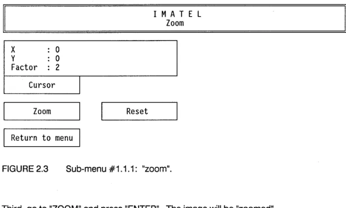
2.1.1.1 Sub-menu #1.1.1: "zoom"

ln order to zoom a particular portion of an image, first move the cursor to the center of the selected portion (the mouse can be used to do sol (figure 2.3).

Second, type the zoom factor that you wish to apply to the image. This factor does not need to be an integer, but should be positive. Also, it can be greater or smaller than one (ex: 1.12; 2.5; 0.5, ... ). [1

x

0

y

0

Factor

2

Cursor

1

Zoom

1

Return to menu

1

Reset

1 MAT E L

Zoom

FIGURE 2.3 Sub-menu #1.1.1: "zoom".

Third, go to "ZOOM" and press "ENTER". The image will be "zoomed".

I[

It is possible to perform a series of zooms on the image by pressing "ENTER" again. The former zoomed image is then taken as the image be zoomed. The zoom factor can also be changed between each consecutive zoom.

ln order to return to the original pixel size select "RESET" and press "ENTER".

IMATEL2.0 /17

Finally, selecting "RETURN TO MENU" and pressing "ENTER", brings the program back to sub-menu #1.1.

2.1.1.2 Sub-menu #1.1.2: "display decimated entire image"

It is very easy to display an image larger than the active window. The image will be decimated, in order to fit into the window.

First, type the name and path of the image (figure 2.4). Second, go to "DO" and press "ENTER". Selecting "RETURN TO MENU" and pressing "ENTER", brings the program back to sub-menu #1.1.

1 MAT E L

Display decimated entire image

Image name

a:inrs.sr8

Do

Return to menu

FIGURE 2.4 Sub-menu #1.1.2: "display decimated entire image".

2.1.1.3 Sub-menu #1.1.3: "display full resolution sub-image"

ln order to display a full resolution image, whether it fits into the active window or not, first type the name and path of the image (figure 2.5). Second, type the origin of the image (or of the sub-image) you want to display. The origin corresponds to the lower left corner of the image or of the sub-image. Third, go to "DO" and press "ENTER".

Selecting "RETURN TO MENU" and pressing "ENTER" brings the program back to sub-menu#1.1.

1 MAT E L

Display full resolution sub-image

Image name

inrs2.sr8

Origin

Do

x

y

0.000

_0.000

Return to menu

FIGURE 2.5 Sub-menu #1.1.3: "display full resolution sub-image".

2.1.1.4 Sub-menu #1.1.4: "save image"

ln order to save the image displayed in the active window, first type the name and path under which you want to save the image. Second, go to "DO" and press "ENTER".

Selecting "RETURN TO MENU" and pressing "ENTER" brings the program back ta sub-menu #1.1.

IMATEL2.0 /19

Il

1 MAT E L

Save image (active window)

Il

Image name

Do

Return to menu

FIGURE 2.6 Sub-menu #1.1.4: "save image".

2.1.2 Sub-menu #1.2: "window tasks"

Sub-menu #1.2 contains 3 tasks allowing to define windows and to select one for display purposes. It is possible to go back to the main menu by selecting "Main menu ... ".

Il

FIGURE 2.7

1 MAT E L

Window tasks

Main menu ...

Choice of active window

Window definition

Choice of active window file

Window option #1

Window option #2

Window option #3

Window option #4

Window option #5

Sub-menu #1.2: "window tasks".

Il

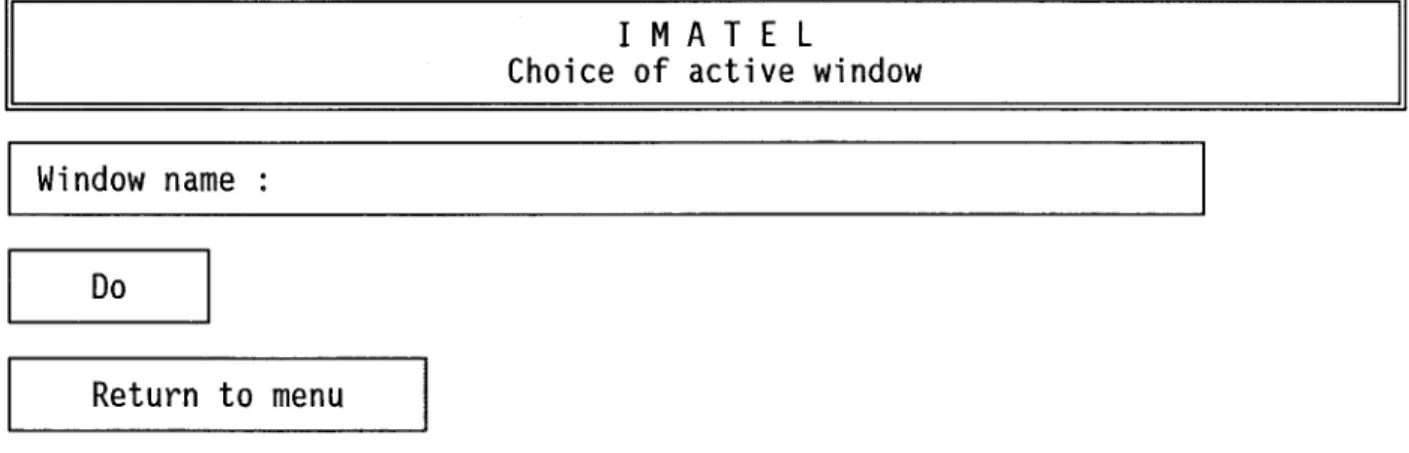
2.1.2.1 Sub-menu #1.2.1: "choice of active window"

Sub-menu #1.2.1 is used essentially to select the active window among those in the active window file. Type the name and path of the (already defined) window you wish as the active window. Go to "DO" and press "ENTER" to confirm your selection. The selected window is then displayed with the last image displayed in this window. Return to sub-menu #1.2 by going to "RETURN TO MENU" and pressing "ENTER".

Il

Window name

Do

1 MAT E L

Choice of active window

Return to menu

FIGURE 2.8 Sub-menu #1.2.1: "choice of active window".

Il

Whether or not the active window does occupy the whole screen, the look-up table relative to the image being displayed in it, is used for the whole screen and thus, for ail other active windows now on the screen. This means that the images in the non-active windows will be displayed with a wrong look-up table CLUT) , unless their LUT is identical to that of the active window.

IMATEL 2.0 /21

2.1.2.2 Sub-menu #1.2.2: "window definition"

Tasks #1.2.2 is used to define ail the windows needed by the user. The only constraint is that the maximum dimensions of a particular window must be smaller then or equal to the maximum allowed by the MATROX 640 A board, that is, 640 pixels by 480 lines. First type the name of the new window. Second, type the origin (Iower left corner) of the window in screen coordinates (640 pixels by 480 lines with origin (0,0) in the lower left corner of the screen).

Then, type the x and y dimensions of the window, remembering the constraints mentionned above.

If you want to display the image within a frame, select a frame color and put the frame "ON", in the "frame color window".

It is also possible to write a title describing the image or the window in the upper part of the window. To do so, select colors for the title and its background and put the title "ON". Three options are available to choose from: the window name, the image name or a free title (user defined).

Once this is done, go to "DO" and press "ENTER". The new defined window is saved in the active window file.

Il

1

Window name

o Limit

Do

FIGURE 2.9

X: 0

255 254 1 MAT E L

Window definition

Y: 0

dX: 640

Return to menu

Sub-menu #1.2.2: "window definition".

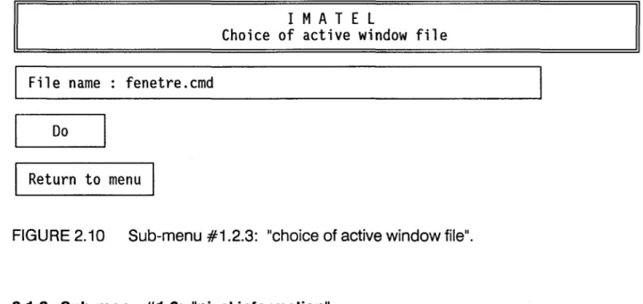
2.1.2.3 Sub-menu #1.2.3: "choice of active window file"

Il

dY: 480

This task allows the user to select the active window file. To create a new window file, or to select an already defined window file, just type the name and path of the (new) windowfile.

Use "DO" to confirm your selection and "RETURN TO MENU" to go back to sub-menu #1.2.

IMATEL 2.0 /23

Il

1 MAT E L

Choice of active window file

Il

File name : fenetre.cmd

Do

Return to menu

FIGURE 2.10 Sub-menu #1.2.3: "choice of active window file".

2.1.3 Sub-menu #1.3: "pixel information"

Task #1.3 is used whenever information is required on a particular pixel. It is possible to type the x and y coordinates of the point, pravided that you know its position relative to the origin of the image (in metric coordinates). However, it is easier to use the mouse by selecting "CURSOR".

Two tables are shown on the dialogue screen. The one on the left is used to enter the names and paths of the image files for which you want informations. As many as 8 image files can be selected simultaneously. As an example, if a color image is displayed on the screen, you may enter the name of the image file obtained by color compression of any 3 image files selected fram the 7 image files corresponding to the 7 spectral bands of a TM scene.

As you move the cursor (with the mouse) on the image, the values of the first line of the right table as weil as those of the x and y coordinates will change.

They represent, from left to right, the LUT index, and the corresponding red, green and blue intensities assigned to the selected pixel, in the case of and image file obtain from color compression of 3 original image files. The original values of ail other spectral

bands appear on the sa me line as the name type in the left table, when the right button (equivalent of DO) of the mouse is pressed.

To leave the task, first return to keyboard input, go to "RETURN TO MENU" and press "ENTER".

Il

X 0 y 0

Cursor

Fil el

File2

Fi 1 e3

File4

File5

File6

File7

File8

Return to menu

1 MAT E L

Pixel information

FIGURE 2.11 Sub-menu #1.3: "pixel information".

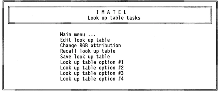
2.1.4 Sub-menu #1.4: "look up table tasks"

Index

190

-1

-1

-1

-1

-1

-1

-1

-1

-1

Il

PIXEL VALUE

R

G B

156

148

156

-1

-1

-1

-1

-1

-1

-1

-1

-1

-1

-1

-1

-1

-1

-1

-1

-1

-1

-1

-1

-1

-1

-1

-1

.

_{out of bounds}

.

ln sub-menu #1.4, 4 tasks are available for LUT operations. Selecting one of those allows editing, saving and recalling LUT, as weil as channel swapping. It is possible to go back to the main menu par selecting "Main menu" and pressing "ENTER".

[1

1 MAT E L

Look up table tasks

Main menu ...

Edit look up table

Change RGB attribution

Recall look up table

Save look up table

Look up table option #1

Look up table option #2

Look up table option #3

Look up table option #4

FIGURE 2.12 Sub-menu #1.4: "look up table tasks".

2.1.4.1 Sub-menu #1.4.1: "edit look up table"

IMATEL 2.0 /25

Il

Task #1.4.1 can be used ta define a complete LUT or ta modify it. The process can be done index value by index value, or for specifie range of values. The range is first selected (maximum 0-255). Then, the red green and blue intensities corresponding ta each index values in the range are given. If, for a particular color, the same intensity (0 ta 255) is given for the lower and higher index value, this means that the intensity of this color will be the same for ail indices within that range.

Il

1111111

From

To

1111111

Index

0

255

Red

0

255

Green

0

255

Blue

0

255

L--_D_o _ _

1 1

Undo

Return to menu

I MAT E L

Edit look up table

Reset

FIGURE 2.13 Sub-menu #1.4.1: "edit look up table".

Il

Use "DO" ta apply the new (or modified) LUT ta the image. If the result is unsatisfactory, it is possible ta come back ta the last modification with "UNOO" or ta the original setting with "R ES ET" .

Ta go back ta sub-menu #1.4, use "RETURN TO MENU".

2.1.4.2 Sub-menu #1.4.2: "change RGB attribution"

Channel swapping is done farly easily with task #1.4.2, by changing the number of the channel attributed ta red, green and blue. It is also possible ta obtain a negative of the displayed image using NEGATIVE, and ta return ta the original image with RESET. A return ta sub-menu #1.4 is done with "RETURN TO MENU".

Il

1111111

_channel

1111111

Red

1

Green

2

Blue

3

Reset

Return to menu

1 MAT E L

Change RGB attribution

If

~I

Negat ive

FIGURE 2.14 Sub-menu #1.4.2: "change RGB attribution".

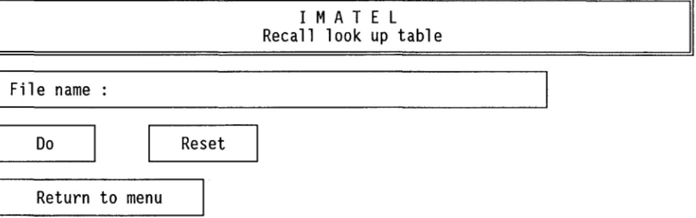
2.1.4.3 Sub-menu #1.4.3: "recaillook up table"

IMATEL 2.0 /27

Il

To recall a LUT from disk, type the name and path of that LUT. The recalled LUT is use to display the current image using "DO". It is possible to come back to the original LUT using RESET and to sub-menu #1.4 using "RETURN TO MENU".

Il

Fil e name :

Do

Return to menu

Reset

1 MAT E L

Recall look up table

FIGURE 2.15 Sub-menu #1.4.3: "recaillook up table".

Il

2.1.4.4 Sub-menu #1.4.4: "save look up table"

ln arder to save a LUT on disk, type the name and path given to the LUT and go to "DO" to confirm that you want to save it under that name and path. A return to sub-menu #1.4 is possible with "RETURN TO MENU".

Il

File name :

Do

Return to menu

1 MAT E L

Save look up table

FIGURE 2.16 Sub-menu #1.4.4: "save look uptable".

2.1.5 Sub,ânu #1.5: "classifications"

Il

The two classification algorithms proposed by IMATEL are very simple. Yet, they may be very useful to classify images (figure 2.17).

The operator has the choice of classifying an image using parallelepipeds centered on a single selected point or parallelepipeds defined by 2 points. Those tasks modify the colors of the active LUT but not the indices of that LUT. A number of the 256 indices may then correspond to the same colar. In order to be able to work with the classified image, task APPLY CLASSIFICATION TO IMAGE must be used. The last task is used essentially to display the themes corresponding to a particular image.

Il

1 MAT E L

Classifications

Main menu ...

Parallelepiped centered on a pixel

Parallelepiped defined by two points

Apply classification to image

Display classes of a classified image

Classification option #1

Classification option #2

Classification option #3

Classification option #4

FIGURE 2.17 Sub-menu #1.5: "classifications".

2.1.5.1 Sub-menu #1.5.1: "parallelepiped centered on a pixel"

IMATEL 2.0 /29

Il

First make sure that an active theme file has been selected, containing the themes to be used for the classification.

With the mouse, move the cursor to a point in the image (figure 2.18) within a "training area", that is an area which can be related to a specifie theme, given field informations. Come back to editing mode and type the name of the corresponding theme. Then, specify how large you want the parallellepiped (cube) araund the chosen point. For this, consider the point in tridimensional spectral space. The red, green and blue values of the point give the coordinates of the point in that space. The SIZE is the distance fram the center of the cube to its si des, in spectral coordinates (0,255). Small cubes should be specified. The result can be displayed with "DO". If it is not satisfactory, it is possible to erase the last modification with "UNDO" and even to go back to the original image with RESET. By selecting appropriate points and size, it should be possible to classify images for hydralogical purposes with a reasonable accuracy. Note that more th an one point may be used to define a particular class.

The modified image can be saved, or only the modified LUT.

x

0

y

₀

Cursor

Theme

Size

1

Do

Return to menu

1 MAT E L

Parallelepipede centered on a pixel

Index

190

R

156

G

148

B

Undo

1 1

Reset

156

FIGURE 2.18 Sub-menu #1.5.1: "parallelepiped centered on a pixel".

2.1.5.2 Sub-menu #1.5.2: "parallelepiped defined by two points"

This task is similar to task #1.5.1, except that the parallelepiped is not necessarily a cube, as it is now defined by two points within the training area (figure 1.19). Remember that an active theme file has to be selected. Assuming you use a mouse, after the first point has been selected, confirm it and come back to the CURSOR window by pressing the left button on the mouse. Then move to the CU RSOR window for the second point, press ENTER and use the cursor to select a second point. After this is done, you may either used the right button to see the result or use the left one to back to the cursor window and then to "DO". The result is displayed when you press ENTER.

IMATEL 2.0 /31

FIGURE 2.19 Sub-menu #1.5.2: "parallelepiped defined bytwo points".

2.1.5.3 Sub-menu #1.5.3: "apply classification to image"

When an image is classified using task #1.5.2 or #1.5.3, the size of the corresponding LUT does not change, even if the maximum number of colors on the screen is 16 instead of 256. Task #1.5.3 reduces the size of the LUT fram 256 to 16, for use in PHYSITEL and HYDROTEL, each LUT index corresponding to a specifie theme. This means that the index of each pixel in the image will range from 0 to 15 in a classified images pracessed by task #1.5.3, whereas it will range fram 0 to 255 for original images (and classified images before processing by task #1.5.3). If there are unclassified pixels in the input image (that is pixels whose colors does not correspond to a theme color, they will be assigned and index value of 0 and will appear in "black".

First give the name and path of the classified (input) image to be processed and then its name after reduction of the LUT indices (output image) (figure 2.20).

Now, in the "classification" window, type the name of each theme in your classified image versus one of the indices 0 to 15. Once this is done, use "DO" to apply the reduction of LUT indices to the input image. The program will look for the color corresponding to a specifie theme in the input image and assign to that color the index corresponding to the theme name in the "class definition" window. The 16 theme name will also be saved in the image header.

It is possible to return to menu #1.5 by selecting "RETURN TO MENU".

Name of input image

Name of output image

#

Theme

#

a

4 1 5 2 6 3 7

Do

Return to menu

1 MAT E L

Apply classification to image

Class definition

Theme

#

Theme

#

Theme

8 12

9 13

la

14

11 15

FIGURE 2.20 Sub-menu #1.5.3: "apply classification to image".

IMATEL 2.0 /33

2.1.5.4 Sub-menu #1.5.4: "display classes of a classified image"

Task #1.5.4 is used to display informations on the various themes of a classified image (figure 2.21). Type the name of the image for which you want information and use "DO" to execute the task and display the information. The name of the various themes of the classifed image will be displayed in the proper window versus their respective index.

1 MAT E L

Display of classes of a classified image

Image name

List of classes

#

Theme

#

Theme

#

Theme

#

Theme

0

4

8

12

1

5

9

13

2

6

10

14

3

7 11

15

Do

Return to menu

FIGURE 2.21 Sub-menu #1.5.4: "display classes of a classified image".

2.1.6 Sub-menu #1.6: "image editing"

Two editing (or utility) tasks are available in IMATEL, RUBBER BAND DRAWING AND GRID (figure 2.22). The first one, RUBBER BAND DRAWING, should facilitates measurement of reach lengths on a river directly on a image. With the second one, GRID, a UTM grid can be superimposed on an image.

Il

1 MAT E L

Image editing

Main menu ...

Rubber band drawing

Grid

Editing option #1

Editing option #2

Editing option #3

Editing option #4

Editing option #5

Editing option #6

FIGURE 2.22 Sub-menu #1.6: "image editing".

2.1.6.1 Sub-menu #1.6.1: "rubber band drawing"

Il

The "RUBBER BAND DRAWING" task (figure 2.23) has been designed to measure lengths on a particular image, the pixel dimensions being known. For instance, it can be used to measure lengths of reaches on a river, or the perimeter of a lake.

Let us assume that a mouse is used for that purpose, choose the "CURSOR" mode and move the cursor to one end of the length you want to measure. Press the right button of the mouse to confirm the initial point. Then move the cursor to another point on the line and press the right button, and so on until you come to the end of the line. At any time, it is possible to erase the last confirm point, by going to the "UNPIN" window and pressing "ENTER". Ali points may be erased, from the last on to the first one. "Curved" line may also be approximated by a series of small linear segments.

Once you have reached the end of the length you want to measure, use "MEASUREMENT" to obtain the length in meters.

IMATEL 2.0

/35

A color may be assigned to any line. To do that select a color index in the active LUT. The line will be drawn using that color, but can be erased using the "UNPIN" function. However, after you use the function "COLORATION", it will not be possible to erase the line in the displayed image.

Finally, "FREE THE CURSOR" before going to another line or selecting "RETURN TO MENU".

As the x,y coordinates of the points and the length between two points are not saved, they should be noted for further use.

Il

x

0

y

0

Cursor

Measurement

Color (0-255) : 0

Coloration

1 MAT E L

Rubber band drawing

Pin

Unpin

Length

0

~

__ F_r_e_e_t_h_e_c_u_r_so_r __

~1 1~

_____

R_et_u_r_n_t_o __

me_n_u ____

~

FIGURE 2.23 Sub-menu #1.6.1: "rubber band drawing".

Il

2.1.6.2 Sub-menu #1.6.2: "grid"

Sub-menu #1.6.2 can be used to superimpose aU.T.M. grid on an image (figure 2.24). To do that, select one point (considered to be a grid node) in the image either by the keyboard or by the mouse. Define the grid interval both in the x and y direction and display the grid with "DO".

It is possible to select any color in the active LUT to display the grid. To do that, select a color index (0-255). The grid can be erased if the function ERA~E is used. When you are satisfied with the grid and its color use "COLORATION", it will not be possible to erase the grid after that function is used.

One may come back to sub-menu #1.6 by "RETURN TO MENU".

Il

1 MAT E L

Il

Grid

X 0 Y 0

Cursor

Step

X : 10

Step

y : 10

Draw

Erase

Color

(0-255) : 0

Coloration

Return to menu

FIGURE 2.24 Sub-menu #1.6.2: "grid",

IMATEL2.0 /37

2.1.7 Sub-menu #1.7: "Ianguage choice"

With IMATEL, the user can choose between ENGLISH and FRANCAIS as the operating language (figure 2.25). A return to the main menu is made possible by MAIN MENU.

[1

1 MAT E L

Language choice

Main menu ...

Français

English

Language option #1

Language option #2

Language option #3

FIGURE 2.25 Sub-menu #1.7: "language choice".

2.2 Main menu (page 2)

Il

More tasks are available on page 2 of the main menu (figure 2.26). With the available input-output formats, it is possible exchange information with EASY-PACE (PCI) and SPANS (TYDAC) , as weil as with PHYSITEL and HYDROTEL. Image enhancement is also possible with HISTOGRAM AND CONTRAST ENHANCEMENT. The color compression algorithm permitting to display color images on IMATEL can be accessed by COLOR COMPRESSION. It is also possible to perform geometric corrections on images using GEOMETRIC CORRECTION. Also, operations on themes are possible through THEME TASKS.

Il

1 MAT E L

Main menu (page 2)

Return to page 1

Input / output ...

Histogram and contrast enhancement

Color compression

Geometrie correction

Theme tasks ...

Option task #1

Option task #2

Option task #3

FIGURE 2.26 Main menu (page 2).

2.2.1 Sub-menu #2.1: "input-output"

Task 2.2.1 is essentially a format transfert task (figure 2.27). The format used in IMATEL is called * .sr8. If the image to be processed is not in the * .sr8 format, it has to be reformated. Two format options are proposed. With the PCIDSK option, it is possible to transfert data from EASY-PACE (PCI) to IMATEL and with the RASTER option, from SPANS (TYDAC) to IMATEL. Other input or output format options are listed by they should be programmed by the user.

No output format is provided, apart the *.sr8 format. However, it should be possible to export image file, if the program by which that image is to be processed can skip the .sr8 header and read the image data.

Il

1 MAT E L

Input / output

Main menu "

Input PCI format

Input format 1

Input format 2

Input format 3

Output format 1

Output format 2

Output format 3

FIGURE 2.27 Sub-menu #2.1: "input-output".

2.2.1.1 Sub-menu #2.1.1: "PCIDSK format"

IMATEL 2.0 /39

Il

This task (figure 2.28) should be used to transfert image data fram PCIDSK format to *.sr8 format. Type the file name of the input file from EASY-PACE and the file name (s) of the output sr8 file. Use "DO" to execute the transfert.

1 MAT E L

PCI format to SR8 format transfert

PCI input fil e

PCI channel number

SR8 output file

(0 : no transfert )

1

0

2

0

3

0

Do

Return to menu

FIGURE 2.28 Transfert fram PCIDSK format to .sr8 format.

2.2.1.2 Sub-menu #2.1.2: "RASTER format"

This task (figure 2.29) should be used to transfert image data fram a general raster format (compatible with SPANS) to *.sr8 format. Type the name of the input file in RASTER format and that of .sr8 output file. Use "DO" to execute the transfert.

IMATEL2.0 /41

1 MAT E L

Transfert from a general RASTER format to *.sr8 format

Input file

Output file

Image size

Origin

Pixel size

1

Return to menu

X 640 X 0

X 1

y 480

Y 0

Y 1

FIGURE 2.29 Transfert fram a general RASTER format to *.sr8 format.

2.2.2 Sub-menu #2.2: "histogram and contrast enhancement"

An enhancement procedure thraugh contrast stretching is available with task #2.2.2 (figure 2.30), as weil as the computation of the histogram of the image.

To do this, it might be better to compute the histogram of the current image first. Go to the histogram window, select COMPUTE and press ENTER to compute the histogram. It is possible to display the histogram on the image by selecting DISPLA y and pressing ENTER. Pressing ENTER again erase the histogram.

Now go to the Contrast Enhancement windows. Type the cutoff and saturation values wished for the image, together with the exponent of the curve. A value of "1" leads to linear stretching. Use DISPLA y and press ENTER to see the enhancement curve and

compare it to the histogram. The curve is erased if you press ENTER again. If you are satisfied with the curve, select DO and press ENTER to execute the task.

1 MAT E L

Histogram and contrast enhancement

Cutoff

0

Contrast enhancement

Saturation

255

Exponent

1.000

00

I~

,1

Oisplay

Reset

Compute

Histogram

I~

,1

0 i s play

Return to menu

FIGURE 2.30 Sub-menu #2.2: "histogram and contrast enhancement".

2.2.3 Sub-menu #2.3: "geometric corrections"

Geometrie corrections are possible with IMATEL. A simple, yet flexible, approach has beentaken, that does not need projection equations.

It is possible to prepare a file containing control points, from informations on a map and on the image. Otherwise, a particular image can be corrected geometrically using an already corrected image or a digitized map. Both images may appear at the same time on the screen if proper windows are selected. Tasks are provided to selected both the image to be corrected (slave image) and the reference image, to select a file to contain control points and to fill that a file with control points from the display (figure 2.31).

Main menu ...

I MAT E L

Geometrie correction

Choice of active window (slave image)

Choice of secondary window (reference image)

Choice of ground control point file

Input of ground control points, image ta image

Resampling (nearest neighbor)

Resampling option #1

Resampling option #2

FIGURE 2.31 Sub-menu #2.3: "geometric corrections".

2.2.3.1 Sub-menu #2.3.1: "choice of active window (slave image)"

IMATEL 2.0 /43

Il

Tasks #2.3.1 is to be used to select the window in which the image to be corrected should be displayed (figure 2.32). Simply type de name and path of the selected window and confirm your choice with DO.

Il

Window name

Do

Return ta menu

I MAT E L

Choice of active window

FIGURE 2.32 Sub-menu #2.3.1: "choice of active window (slave image)".

Il

2.2.3.2 Sub-menu #2.3.2: "choice of secondary window (reference image)"

Task #2.3.2 is to be used to select the window in which the reference image (or digitized map) should be displayed (figure 2.33). Simply type the name and path of the selected window and confirm your choice with DO.

Il

1 MAT E L

Choice of secondary window

Il

Window name

Do

Return to menu

FIGURE 2.33 Sub-menu #2.3.2: "choice of secondary window (reference image)".

~.2.3.3 Sub-menu #2.3.3: "choice of ground control point file"

A filename under which the control points chosen in task 2.3.3 "INPUT OF GROUND CONTROL POINTS", will be saved must be chosen or defined before task 2.3.3 is used. to do that, type the name and path of the file in which control points will be saved, select DO and press "ENTER".

IMATEL 2.0 /45

1 MAT E L

Choice of ground control point file

Filename

ctr.cmd

1

Return to menu

FIGURE 2.34 Sub-menu #2.3.3: "choice of ground control point file".

2.2.3.4 Sub-menu #2.3.4: "input of ground control points image to image"

Task 2.3.4 (figure 2.35) is used to input the control points needed to perform a geometric correction on a particular image. The chosen points should be distributed as much as possible over the image and their number should be at least 6.

1 MAT E L

Input of ground control points, image to image

SLAVE IMAGE

Point

# 1

1 1

Remove

1

X

0

»»

Record

_»»

1

X:

y ₀

_Y:

Cursor

REFERENCE IMAGE

X

0

»»

Record

_»»

1

X:

Y

0

Y:

Cursor

Return to menu

1 1

Model

FIGURE 2.35 Sub-menu #2.3.4: "input of ground control points image to image".

The identification number of the selected point appears in the upper part of the menu. It is possible to go up (right pointing arrow) and down (Ieft pointing arrow) in the list of control points.

Note that either the keyboard or the mouse can be used to enter the coordinates of the control points. Let us assume that you start with the image to be corrected (slave image). Using the mouse, you select a point on the image that you want to be control point number 1. While the cursor is being moved over the image, the coordinates X and

y change. When you are satisfied with the position of the point, leave the CURSOR mode, and go to RECORD and press ENTER to register the coordinates of the first point in the slave image.

IMATEL 2.0 /47

Then go to the CURSOR function associated with the reference image to come back in CURSOR mode on the reference image and select and RECORD the corresponding point on that image.

Once the coordinates of the first control point have been registered on both images, go to the next control point with the right pointing arrow, and so on until ail control points have been selected. It is also possible to remove points using REMOVE.

As the keyboard can be used to input the X and Y coordinates of a point, that means that the points on the slave image can be chosen directly on the screen using the mouse, whereas the corresponding controls points of the "reference" may be read on a map and input with the keyboard.

When the set of control points is completed, the parameters of the polynomial equation used to make the correction are computed by the function MODEL.

2.2.3.5 Sub-menu #2.3.5: "resampling"

Resampling of an image by nearest neighbour to perform a geometric correction is done by task 2.3.5 (figure 2.36). Type first the name and path of the image to be corrected and then the name and path of the image after correction.

The size (X and Y) of the pixels in the corrected image is given as is the lower left corner and upper right corner of the image after correction. Those points should be taken on the reference image.

To execute the task go to DO and press ENTER.

Il

INPUT IMAGE

1

Fil e name

OUTPUT IMAGE

Fil e name :

Pixel size

Lower left corner

Upper right corner

1

Return to menu

X: 1

X: 0

X: 0

1 MAT E L

Image resampling

Y: 1 Y: 0 Y: 0

FIGURE 2.36 Sub-menu #2.3.5: "resampling".

2.2.4 Sub-menu #2.4: "color compression"

Il

The idea behind the coler compression algorithm is to be able to display and save a 8 bit coler image made out of three distinct single band image files, without loosing to much of the original 3 x 8-bit color image, as far as eye perception is concerned. In other words, the algorithm compresses three images files leading to a possibility of 16 M colors to one image file, with a maximum of 256 colors, that occupies only one third of the original space needed to store the three initial files.

Type first the names of the input image (figure 2.37) files assigned to red, green and blue respectively. If a constrast enhancement (sub-menu 2.2) is wished for any of those

IMATEL2.0 /49

image files, give the cutoff, saturation and exponent values. The image is left unchanged if the values are 0,255 and 1, respectively.

Next, informations for the compression process have to be given.

It is possible to accelerate the compression process, if only one pixel out of a certain number is used to compute the statistics. So a sampling factor is possible. A sampling factor of 1 means that ail pixels are taken into account, whereas a value of 10, for instance, means that 1 out of 10 is used.

The maximum number of colors after the color compression must also be given. If the value 256 is typed, that means that ail colors in the LUT will be used to display the image. However a few, or many, LUT indices may be kept available for other operations on the images (rubber band drawing, classification, ... ). Of course it is possible to keep the maximum of 256 colors for the image, and to choose the colors from the available LUT to perform other operations.

A initial 3 x 8-bit color may appear only a given to a few pixels on 100 000 and be unnoticeable on the screen, whereas many pixels with relatively close 3 x 8-bit colors may be obtained. The next function (minimum number of pixels by color) allows to take care of the original color population (number of pixels for each initial colors of groups of very close colors within a R-G-B cube in color space). Type the minimum number of pixels by col or, on a population of 100 000 pixel, that you want to have to assign a color to that group of pixels.

Finally, type the name of the output file and select "DO" to compute the color compression.

Il

1 MAT E L

Color compression

Channel

Name of input file

Red

Green

Blue

Sampling facteur

Maximum number of color

Maximun number of pixel by color

Name of output file

Do

Return to menu

1

256

1

Cutoff

a

a

a

FIGURE 2.37 Sub-menu #2.4: "color compression".

2.2.5 Sub-menu #2.5: "theme tasks"

Il

Saturation

Exponent

255

1

255

1

255

1

by 100 000 pixels

Two theme tasks are available (figure 2.38). The first one is there only for the selection of the active theme file. The theme in each theme file can be defined with the second task (theme editing).

Il

Main menu ...

1 MAT E L

Theme tasks

Choice of active theme file

Theme editing

Theme option #1

Theme option #2

Theme option #3

Theme option #4

Theme option #5

Theme option #6

FIGURE 2.38 Sub-menu #2.5: "the me tasks".

2.2.5.1 Sub-menu #2.5.1: "choice of active theme file"

IMATEL 2.0 /51

Il

Type the name of the theme file to be used as active theme file (figure 2.39). Then go to DO and press ENTER.

Il

1 MAT E L

Choice of active theme file

Il

File name : imatel.thm

Do

Return to menu

FIGURE 2.39 Sub-menu #2.5.1: "choice of active theme file".

2.2.5.2 Sub-menu #2.5.2: "theme editing"

A maximum of 15 themes may be defined with task 2.5.2 (figure 2.40).

Theme number "0" is not editable. Ali non-classified pixels will be assigned to that theme number and will appear in black (0, 0, 0) in the classified image.

Using the arrows, you can go up and down in the theme list (maximum value 15). For each theme number, specify a code name and a description of that theme, together with the red, green and blue values with which you want to display it.

When those informations are completed for a theme number, select "WRITE TO FILE" to save the information in the theme file.

Il

Number :

a

1

Name

Description

Red value

Green value

Blue value

Write to

fil

e

Return to menu

NIL

NIL

a

a

a

1 MAT E L

Theme editing

FIGURE 2.40 Sub-menu #2.5.2: "theme editing".

Il

PART 3

PART 3 HINTS ON THE USE OF IMATEL

3.1 Introduction

The objective of Part 3 is to give hints on the way tasks available in IMATEL 2.0 can be used to obtain specifie informations.

3.2 Determination of river characteristics

IMATEL (version 2.0) can be used to obtain informations on river characteristics, needed in the HYOROTEL files *.NOS and *.TRO.

ln particular, task "Rubber band drawing" (sub-menu #1.6.1) can be used to estimate reach lengths and x-y coordinates of their upstream and downstream ends. To do that, display an image of the region (watershed) of interest. That image can be classified or not. Put the cursor first on the position of the river that you consider as the outlet. That position might coïncide with a gaging station. Do as required in sub-menu #1.6.1 going upstream along the river to defined the first river reach. In doing that, note the x-y coordinates of the downstream and upstream end of the reach as weil as its length. Repeat these operations for ail the reaches that you consider as such. Please note that the homogeneous hydrological units (HHU's) defined in PHYSITEL and used in HYOROTEL, must drain into a river reach. In other words, no drainage from HHU to HHU is allowed, each one has to be related to a river reach. This is true only when HHU's are not built up of only one cell. When the user chooses to work with cells and not with HHU's, that restriction is not applicable. The cells can drain into each other. Widths of river channels may also be estimated. For large widths, the same task, "Rubber band drawing", can be used. For smaller width, it might be better to use the task "pixel information" (sub-menu #1.3). The methodology to use that task is still under development. It is based on the information carried by mixed pixels. Using an unclassified image, choose a spectral band (or a few bands) in which the contrast

IMATEL 2.0 /55

between water, on one side, and soil and vegetation on the other, is good. Start looking at pixel values on the land on one side of the river, at least 4 or 5 pixels from the river. Then, going from pixel to pixel, cross the river and continue on the other side for at least 4 or 5 pixels. Note ail pixel values and make a graph of that cross section. Starting with larger river reaches, identify water, land and vegetation pixels. Then, using those values, try to estimate the relative proportion of water and land or vegetation present in the mixed pixels corresponding to the water-Iand (vegetation) line. As an example, let us assume that the pixels are 20 m in size. If the mixed pixel on the left bank contain 20% of water, 2 pure water pixels can be identified and the right bank mixed pixel contains 70% of water, then the width of the river channel will be 58 m.

Finally, elevations of reach ends could be estimated using a detailed digital elevation model (DEM). Such a model can be displayed in PHYSITEL.

IMATEL 2.0 / A.57

APPENDIX A USER'S DEFINED FUNCTIONS

HOW TO INSERT USER'S DEFINED FUNCTION TO IMATEL

The goal of this section is to explain how to add new capabilities to IMATEL. Adding a function to IMATEL is really easy, you don't need to recompile IMATEL or link your function to the rest of IMATEL because your function is a complete program by itself. The only thing that you have to worry about is the na me of your program which is predefined by IMATEL. Your program has the responsability of managing ail the input/output it requires. The whole process can be divided according to the four following steps:

1. edit file "FIMATEL.F";

2. locate the menu where you want to insert your program; 3. note the name that your program should take;

4. write or rename your program. Step 1: Edit file "FIMATEL.F"

- Use any text editor to edit file "FIMATEL.F".

Step 2: Locate the menu where you want to insert your program

- Locate the menu in the language you want, the first half is the FRENCH part while the second describes the ENGLISH menus. You can choose any menu item with the string "option #" followed bya number. You sould insure that the item does not have a program associated with it. We will come back on this later.

- Note the letter at the beginning of the line.

- Match that letter with the letter in the DIALOGUE structure below the menu.