Analyse fréquentielle régionale non stationnaire des crues à des sites non jaugés.

(1)

Université du Québec INRS Eau, Terre et Environnement

ANALYSE FRÉQUENTIELLE RÉGIONALE NON STATIONNAIRE DES CRUES À DES SITES NON JAUGÉS

Par Martin Leclerc

Mémoire présenté pour l'obtention du grade de Maître ès sciences (M.Sc.)

en sciences de l'eau

Jury d'évaluation

Président du jury et examinateur interne Salaheddine El Adlouni

Examinateur externe

Directeur de recherche

INRS Eau, Terre et Environnement S. Rocky Durrans

Department of Civil and Environmental Engineering University of Alabama

Taha B.M.J. Ouarda

(2)

(3)

SECTIONl

LA SYNTHÈSE

(4)

(5)

RÉSUMÉ

L'analyse fréquentielle régionale des crues est couramment utilisée pour estimer le risque de crue à un site où peu ou pas d'information est disponible sur les débits de pointe. Cette approche nécessite 1 'hypothèse de stationarité des crues. Dans ce mémoire, une nouvelle méthode est présentée afin de procéder à une analyse fréquentielle régionale des crues à des sites non jaugés lorsque l'hypothèse de stationarité n'est pas vérifiée. Des modèles locaux non stationnaires sont utilisés pour estimer le risque de crue aux sites jaugés. Cette information est ensuite utilisée de pair avec les caractéristiques physiographiques et météorologiques des bassins versants de façon à définir un voisinage hydrologique pour le site non jaugé par l'analyse canonique des corrélations (ACC). Un modèle de régression multiple est développé à l'intérieur de ce voisinage. La méthode proposée a été testée à partir d'un groupe de stations de jaugeage des débits situées dans le sud-est du Canada et le nord-est des Etats-Unis et qui présentent un signal de non stationarité. Les résultats indiquent que le développement d'un modèle de régression multiple au moyen de 2 variables explicatives (incluant l'aire du bassin versant) mène à de bonnes estimations des quantiles de crue régionaux et non stationnaires de temps de retour 5 et 100 ans pour la fin de la période d'observation historique (racine de l'erreur quadratique relative moyenne de 38.2 % et 60.8 % respectivement). L'utilisation de l'ACC pour la définition du voisinage hydrologique n'a pas donné de meilleurs résultats. Le nombre total de sites (29) est faible et, conséquemment, la taille des voisinages hydrologiques est trop petite pour développer de bons modèles de régression à l'intérieur de ceux-ci. La comparaison des quantiles de crue régionaux et non stationnaires avec les résultats stationnaires montre que le fait d'ignorer une tendance des crues printanières d'un site non jaugé peut mener à une sous-estimation ou surestimation considérable des quantiles de crue pour ce site .

!1~?

; . ! . / 1 i '\, .'

1 .' 1; _..

~

Étudiant Directeur de recherche

Note.' Ce résumé sert aussi de résumé en français pour l'article de la section 2.

(6)

(7)

REMERCIEMENTS

Je remercie:

Mon directeur de recherche, monsieur Taha Ouarda, pour le support et la confiance qu'il a manifesté à mon égard pendant mes deux années de maîtrise en sciences de l'eau;

Mes camarades étudiantes et étudiants à la maîtrise, pour la richesse des discussions et des expériences vécues depuis le stage de terrain de septembre 2004 jusqu'à aujourd'hui. Je tiens à souligner particulièrement l'aide de Véronique Jourdain avec qui j'ai travaillé en étroite collaboration tout au long de ma recherche;

Monsieur Salaheddine El Adlouni, associé de recherche dans l'équipe de mon directeur, pour l'aide fournie au niveau de l'analyse fréquentielle locale non stationnaire.

(8)

(9)

TABLE DES MATIÈRES

SECTION 1 : LA SYNTHÈSE ... .111

RÉSUMÉ ... V REMERCIEMENTS ... VII LISTE DES FIGURES ... XI INTRODUCTION ... 1 CHAPITRE 1 ... 3 CONTRIBUTION DE L'ÉTUDIANT ... 3 CHAPITRE 2 ... 9 SITUATION DE LA CONTRIBUTION ... 9 CONCLUSION ... Il APPENDICE A ... 13

LISTE DES RÉFÉRENCES ... 31

SECTION 2 : L' ARTICLE ... 33

RÉSUMÉ EN FRANÇAIS ... 35

NON-STATIONARY REGIONAL FLOOD FREQUENCY ANALYSIS AT UNGAUGED SITES ... 37

(10)

j

(11)

LISTE DES FIGURES

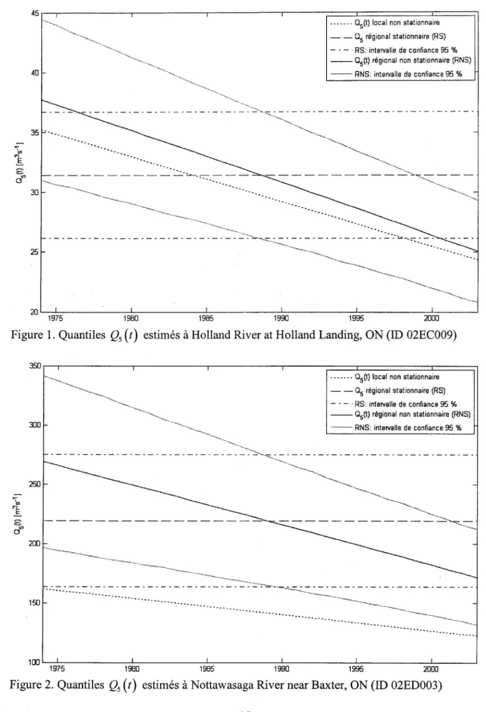
Figure 1. Quantiles Qs

(t)

estimés à Holland River at Holland Landing, ON (ID 02EC009) ... 15

(t)

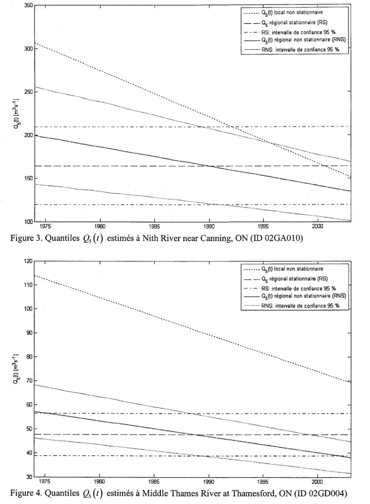
estimés à Nottawasaga River near Baxter, ON (ID 02ED003) ... 15

(t)

estimés à Nith River near Canning, ON (ID 02GA010) ... 16

(t)

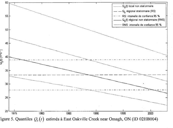
estimés à Middle Thames River at Thamesford, ON (ID 02GD004) 16 Figure 5. Quantiles Qs

(t)

estimés à East Oakville Creek near Omagh, ON (ID 02HB004) ... 17

(t)

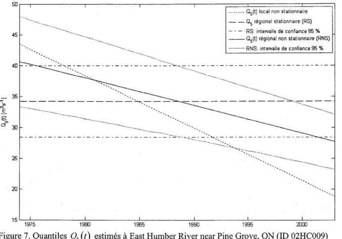
estimés à Grindstone Creek near Aldershot, ON (ID 02HB012) ... 17

(t)

estimés à East Humber River near Pine Grove, ON (ID 02HC009) .. 18

(t)

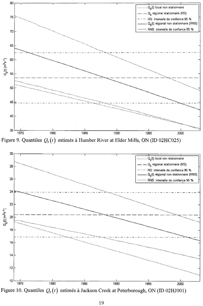
estimés à Duffins Creek above Pickering, ON (ID 02HC019) ... 18

(t)

estimés à Humber River at Eider Mills, ON (ID 02HC025) ... 19

(t)

estimés à Jackson Creek at Peterborough, ON (ID 02HJ001) ... 19

Figure Il. Quantiles Qs

(t)

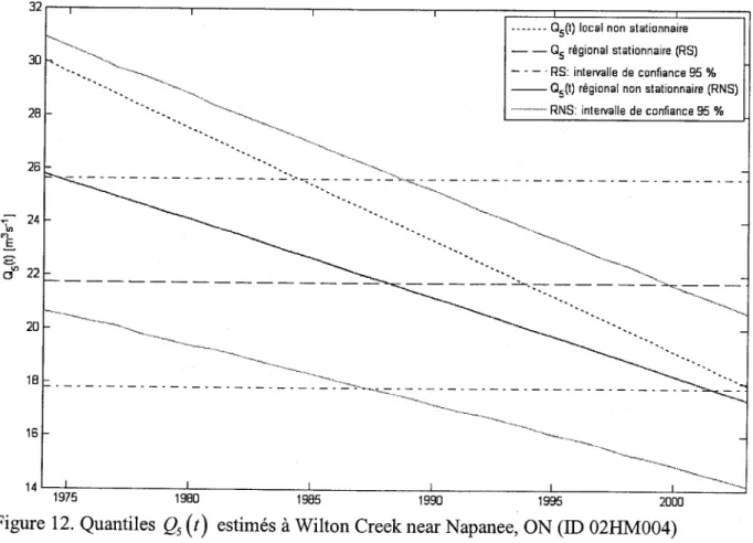
estimés à Moira River near Deloro, ON (ID 02HL005) ... 20

(t)

estimés à Wilton Creek near Napanee, ON (ID02HM004) ... 20

(t)

estimés à Dartmouth (rivière) en amont du ruisseau du Pas de Darne, QC (ID 01BH005) ... 21

(t)

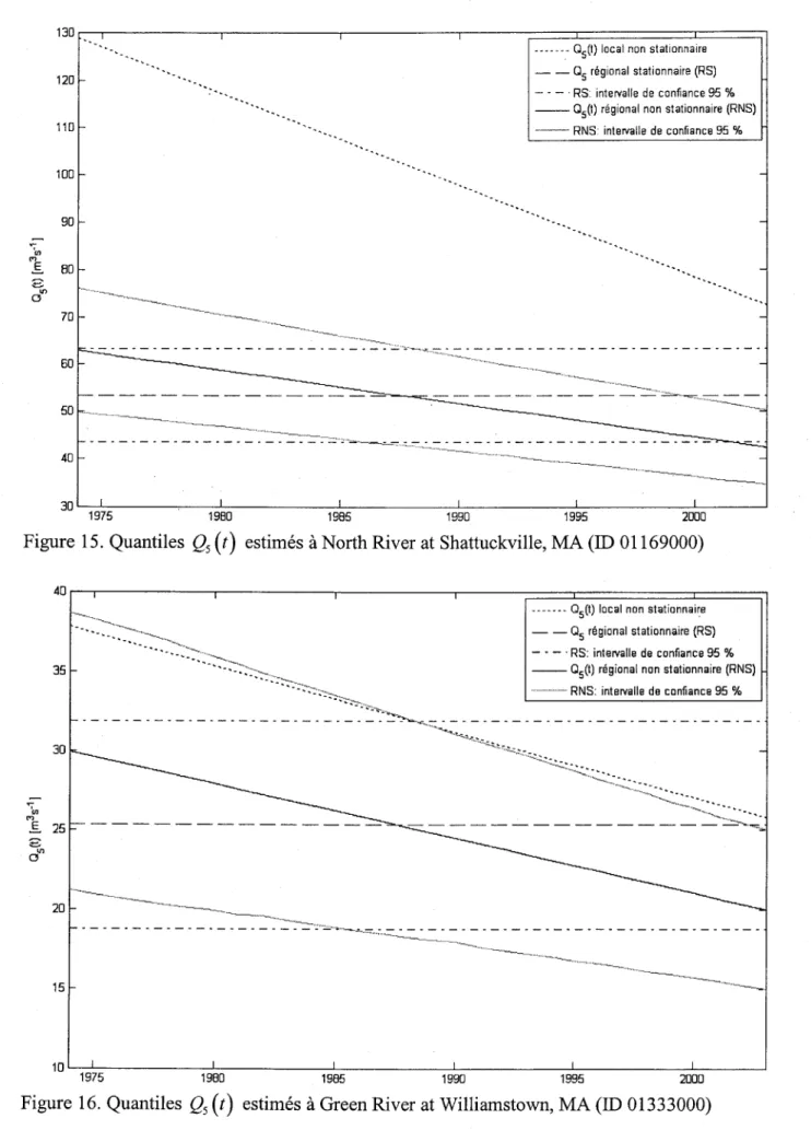
estimés à Kinojevis (rivière) à Cléricy, QC (ID 02JB013) ... 21

(t)

estimés à North River at Shattuckville, MA (ID 01169000) ... 22

(t)

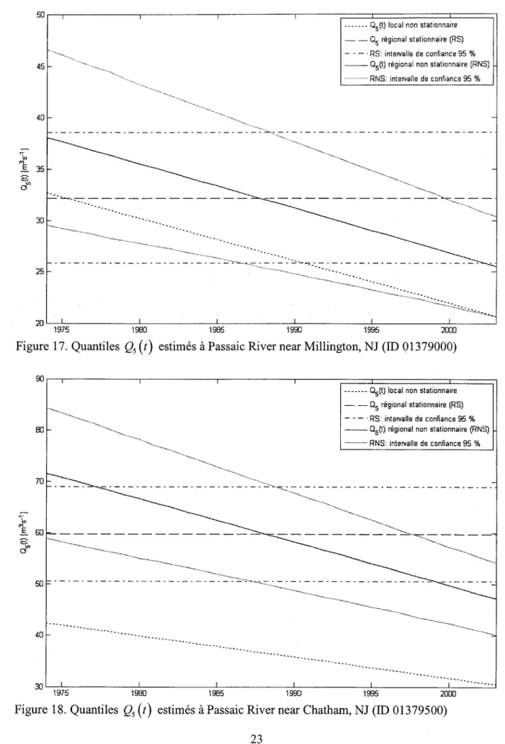
estimés à Green River at Williamstown, MA (ID 01333000) ... 22

(t)

estimés à Passaic River near Millington, NJ (ID 01379000) ... 23

(t)

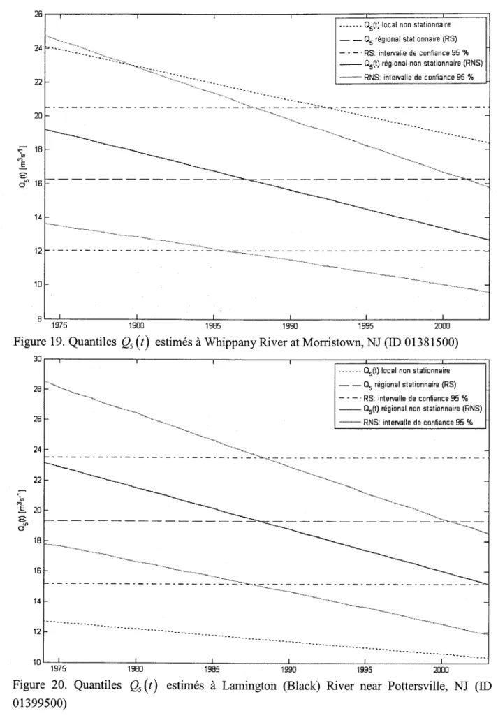
estimés à Passaic River near Chatham, NJ (ID 01379500) ... 23

(t)

estimés à Whippany River at Morristown, NJ (ID 01381500) ... 24

(t)

estimés à Lamington (Black) River near Pottersville, NJ (ID 01399500) ... 24

(t)

estimés à Raritan River at Manville, NJ (ID 01400500) ... 25

(t)

estimés à Raritan River below Calco Dam at Bound Brook, NJ (ID 01403060) ... 25

(t)

estimés à Bush Kill at Shoemakers, PA (ID 01439500) ... 26

(t)

estimés à West Branch Susquehanna River at Bower, PA (ID 01541000) ... 26

(t)

estimés à Spring Creek near Axemann, PA (ID 01546500) ... 27

(t)

estimés à Spring Creek at Milesburg, PA (ID 01547100) ... 27

(12)

(t)

estimés à Bald Eagle Creek bl Spring Creek at Milesburg, PA (ID 01547200) ... 28 Figure 28. Quantiles Qs

(t)

estimés à Monocacy River at Jug Bridge near Frederick,

MD (ID 01643000) ... 28 Figure 29. Quantiles Qs

(t)

estimés à Bear Creek near Muskegon, MI (ID 04122100) ... 29

(13)

INTRODUCTION

Le présent projet de maîtrise consiste à développer une méthode d'estimation des crues de récurrence donnée (par exemple 100 ans, c'est-à-dire susceptible de se produire en moyenne une fois au cours d'une période de 100 ans) dans le cas d'un bassin versant non jaugé (ne disposant pas de station de mesure des débits en rivière) dont le régime hydrologique varie dans le temps (c'est-à-dire est non stationnaire). L'estimation des crues de récurrence est importante à des fins, par exemple, de construction d'un barrage hydroélectrique ou de cartographie des zones inondables. Depuis les premiers travaux de Dalrymple (1960) dans le domaine, plusieurs méthodes se situant en dehors du cadre non stationnaire ont été préconisées. L'originalité du projet est de situer l'analyse à l'intérieur de ce contexte.

Clairement, le projet vise à répondre à la question suivante: Comment estimer les quantiles de crue d'un bassin versant non jaugé dans un cadre non stationnaire?

Une revue de littérature a d'abord été réalisée afin d'identifier les méthodes existantes d'analyse régionale non stationnaire des crues. Cette revue a nourri la réflexion vers le développement d'une méthode dans le cas d'un bassin versant non jaugé. Le modèle retenu pour le présent projet est une extension directe au cadre non stationnaire d'une procédure d'estimation régionale existante pour les sites non jaugés (voir Girard et al., 2000; Ouarda et al., 2001). Des bases de données hydrométriques, météorologiques et physiographiques décrivant les caractéristiques de bassins versants du sud-est du Canada et du nord-est des États-Unis ont été développées afin de tester le nouveau modèle. Nous avons utilisé une procédure de validation croisée afin de comparer les quantiles de crue estimés localement avec ceux fournis par le modèle. Une procédure similaire a aussi été employée

à

des fins de comparaison du nouveau modèle avec le modèle traditionnel stationnaire.

Cette section

«

Synthèse» du mémoire de maîtrise est divisée de la façon suivante. Le chapitre 1 précise la contribution de l'étudiant par rapport aux travaux ayant mené à l'article scientifique de la deuxième section. Le chapitre 2 situe cette contribution par rapport à d'autres articles scientifiques traitant de l'analyse fréquentielle des crues.

(14)

j

(15)

CHAPITRE 1

CONTRIBUTION DE L'ÉTUDIANT

La revue de littérature du projet de maîtrise a été réalisée en entier par l'étudiant à l'hiver 2005. Les résultats de cette recherche sont présentés dans la partie « Introduction and literature review » de l'article de la deuxième section. Les articles de Cunderlik et Bum (2003) et de Cunderlik et Ouarda (2006) constituent, en effet, la liste exhaustive des méthodes d'analyse régionale non stationnaire des crues que la revue a permis d'identifier. Tel que précisé dans l'article, la revue de lihérature a mené au constat de l'absence d'un exemple documenté d'analyse fréquentielle non stationnaire des crues à des sites non jaugés.

L'étudiant a travaillé au développement d'un nouveau modèle principalement à l'automne 2005. La décision finale quant au choix du modèle a été prise au début de l'hiver 2006, d'un commun accord entre l'étudiant et son directeur de recherche. Le modèle a été finalisé au printemps 2006, le processus allant de pair avec la sortie des résultats de la validation. La version finale du modèle est décrite dans la partie 3 «Non-stationary regional model» de l'article. Tel que mentionné en introduction, le modèle retenu est une extension directe au cadre non stationnaire d'une procédure d'estimation régionale existante pour les sites non jaugés. Ainsi, il utilise des méthodes décrites dans des articles scientifiques antérieurs. Ces méthodes sont présentées dans la partie 2 «Theoretical background» de l'article.

La première étape du modèle (partie 3.1 «Flood frequency analysis at gauged sites ») consiste à estimer localement les quantiles de crue d'un certain nombre de bassins versants jaugés. Pour ce faire, le modèle GEV (generalized extreme-value) non stationnaire de El Adlouni et al. (2006) est utilisé (voir partie 2.1 «Non-stationary at-site flood frequency analysis »).

L'étape 2 du modèle (partie 3.2 « Neighborhood identification using CCA ») correspond à l'identification d'un groupe de bassins versants jaugés ayant un régime hydrologique suffisamment similaire au site non jaugé. Cette identification se fait via l'analyse canonique des corrélations (ACC). Quant à l'étape 3 du modèle (partie 3.3 « Information transfer »), elle

(16)

correspond à l'estimation des quantiles de crue au site non jaugé par transfert de l'information disponible via un modèle de régression multiple. Ces deux étapes sont similaires à celles qu'on retrouve dans le modèle traditionnel stationnaire. Ainsi, la théorie sous-jacente (voir partie 2.2

«

Delineation ofhydrologic neighborhoods ») est inspirée de l'article de Ouarda et al. (2001) dans lequel les auteurs ont appliqué le modèle traditionnel stationnaire à un ensemble de bassins versants du sud de l'Ontario. Il faut aussi mentionner que dans une recherche subséquente Girard et al. (2000) ont apporté une modification à ce modèle pour améliorer la définition du voisinage hydrologique. Le présent projet de maîtrise incorpore cette suggestion. En résumé, au niveau du modèle, la contribution de l'étudiant est d'avoir adapté le modèle traditionnel (Girard et al., 2000; Ouarda et al., 2001) en remplaçant les distributions statistiques stationnaires par le modèle GEV non stationnaire décrit par El Adlouni et al. (2006). Il en résulte que les étapes 2 et 3 du nouveau modèle, en plus d'être appliquées pour chaque temps de retour T doivent aussi l'être pour chaque pas de temps t étant donné que le risque hydrologique peut varier dans le temps. Les quantiles de crue pour le bassin versant non jaugé prennent donc la formulation suivante: Qr

(t)

(ils sont conditionnels au temps).

Le nouveau modèle a été testé à partir de données réelles. La méthodologie retenue par l'étudiant est décrite dans la partie 5

«

Study methodology» de l'article. Les bases de données hydrométriques, météorologiques et physiographiques décrivant les caractéristiques de bassins versants du sud-est du Canada et du nord-est des États-Unis ont été développées conjointement par Véronique Jourdain, étudiante à la maîtrise en sciences de l'eau au centre ETE, et l'étudiant. Leurs projets de maîtrise respectifs nécessitant l'utilisation d'une telle base de données, ils ont jugé opportun de conjuguer leurs efforts. Madame Jourdain s'est occupée de recueillir et de traiter les données hydrométriques et physiographiques pour les bassins versants du sud-est du Canada et l'étudiant a fait de même pour les bassins versants du nord-est des États-Unis. L'étudiant s'est aussi chargé de recueillir et de traiter les données météorologiques pour l'ensemble du territoire à l'étude (incluant le couplage entre les stations hydrométriques et les stations météorologiques). Le travail de construction des séries de crues printanières et d'implémentation/application du test retenu pour la vérification des hypothèses du modèle a été réalisé conjointement par madame Jourdain et l'étudiant. Tous les faits saillants concernant la construction de la base de données sont décrits dans la partie 4

«

Case study » de l'article. Quant au test pour la vérification des hypothèses du modèle,

«

trend-free pre-whitening

(17)

(TFPW) procedure >> de Yue et aL. (2002, 2003), il est décrit dans la partie 5 < Study methodology >. Il permet de vérifier les hypothèses d'indépendance et de non stationnarité de premier ordre des séries de crues printanières servant à tester le nouveau modèle. La non stationnarité de premier ordre signifie que seulement le paramètre de position des séries varie dans le temps. La variance et tous les autres moments d'ordre supérieur sont supposés constants.

L'analyse fréquentielle locale non stationnaire (étape 1 du nouveau modèle) étant nécessaire à leurs projets respectifs, madame Jourdain et l'étudiant ont maintenu leur association pour cette étape. Monsieur Salaheddine El Adlouni, associé de recherche dans l'équipe de monsieur Taha Ouarda, nous a aidés par ses commentaires et suggestions pour l'ajustement des paramètres du modèle GEV non stationnaire.

L'étudiant a produit seul les résultats pour les étapes 2 et 3 du modèle (identification du voisinage hydrologique et transfert d'information via une régression multiple), incluant tous les tableaux et graphiques se trouvant dans I'article. À des fins de comparaison du nouveau modèle avec le modèle traditionnel stationnaire, une analyse fréquentielle locale stationnaire utilisant la même base de données que celle mentionnée précédemment s'avérait nécessaire. L'étudiant a pu bénéficier du fait que Véronique Jourdain avait déjà effectué ce travail pour son propre projet de maîtrise. I1 s'agit d'une procédure automatisée s'effectuant à I'aide de programmes informatiques. La contribution de l'étudiant au niveau de cette analyse se limite donc à une discussion et à une récupération des résultats auprès de madame Jourdain. Enfin, l'étudiant a produit seul les résultats de la comparaison entre le nouveau modèle et le modèle traditionnel stationnaire.

L'interprétation, la discussion et les conclusions de l'étudiant entourant l'ensemble des résultats se trouvent dans les parties 6 et 7 de I'article (< Results and discussion > et << Conclusions )) respectivement). Les discussions que l'étudiant a eues avec son directeur de recherche lui ont permis de mieux préciser certains éléments de la conclusion.

La première version de l'article scientifique se trouvant dans la section 2 de ce mémoire a été rédigée entièrement par l'étudiant. Des corrections et modifications ont été apportées par le directeur de recherche.

(18)

Suite au dépôt initial du présent mémoire et à la lecture des rapports des examinateurs,

l'étudiant

prend bonne note des améliorations

suggérées

en vue de la publication

de I'article

dans le Journal of Hydrology.

Dans la partie 3.1 < Flood frequency analysis at gauged sites >, I'algorithme MCMC (Monte Carlo par chaînes de Markov) est utilisé pour calculer des estimateurs des paramètres du modèle GEV non stationnaire. Afin de signaler la taille de la chaîne de Markov et le temps de chauffe utilisés, les phrases suivantes sont à ajouter : < Markov chains of size 25,000 are constructed. The burn-in period is 10,000. >. Elle s'insère au bas de la page 43 après la phrase : <t The MCMC procedure of El Adlouni et al. (2006) is used. y

Au niveau de l'équation (15) (partie 3.3 < Information transfer >>, page 45),le terme de gauche de l'égalité, Qr(t), varie en fonction du temps / alors qu'aucune quantité du terme de droite ne varie explicitement en fonction du temps. À d"s fins de clarification, cette partie de l'article est à réécrire de la façon suivante à partir de la deuxième phrase :

The problem is typically described using the power-form equation

Q , ( t ) = r o ( t ) . X ! ) . . .

Y n Q )

. r"(t)

where yo(t),rr(t),...,y,(t) are model parameters and e(t) a

(r)

random error term. Many

dffirent procedures are available to estimate the model parameters y,(t). One common procedure is to linearize Equation (Ia) through a logarithmic transformation

l o s Q ,

( r ) = lo g

_{r o ( t ) + y r ( t ) l o g X , + . . . +}

_{r , ( t ) l o g x , + e}

( r )

(2)

and then to estimate the model parameters in Equation (15) using an ordinary least-squares technique. This procedure is used here for each time step t.

Aussi, dans la même optique, I'avant-avant-dernière phrase de la partie 3.2 < Neighborhood identification using CCA ) à la page 45 est à bonifier de la façon suivante : < Some of those

(19)

variables can reflect the presence of non-stationarity in flood characteristics and vary through time (implicitly shown here: X (t)= X ). v

Enfin, il a aussi été suggéré d'ajouter les graphiques _{des quantiles QrU) estimés pour des sites} autres que la station 018H005 - Dartmouth (rivière) en amont du ruisseau _{du Pas de Dame, QC} (voir figure 2, page 63, bas de la page 53 dans le texte de I'article). L'appendice A contient les graphiques correspondants pour les 29 sites de l'étude de cas (voir partie 4 < Case study > de I'article).

(20)

(21)

CHAPITRE 2

SrruarroN DE LA coNTRIBUTIoN

La revue de littérature effectuée à l'hiver 2005 a permis de mettre en lumière que I'estimation des quantiles de crue pour un bassin versant non jaugé dans un cadre non stationnaire est un sujet n'ayant pas fait l'objet d'un article scientifique jusqu'à maintenant. La contribution de l'étudiant se concentre spécifiquement sur cette question.

Les articles scientifiques traitant de I'analyse régionale non stationnaire des crues sont peu nombreux. Deux ont été identifiés : celui de Cunderlik et Bum (2003) et celui de Cunderlik et Ouarda (2006). Cependant, dans chacun de ces articles, les études de cas présentées concernent des bassins versants pour lesquels des séries de débits mesurés sont disponibles localement. À l'intérieur de la méthodologie utilisée pour I'obtention des résultats, ces séries sont utilisées directement ou mises en commun avec celles de d'autres bassins versants de façon à améliorer l'estimation des quantiles au site d'intérêt. On ne présente pas de résultats pour un bassin versant non jaugé. En présentant de tels résultats avec une méthodologie associée, le projet de mémoire s'inscrit dans la continuité de ces articles.

De plus, l'étudiant apporte une contribution qui représente une extension par rapport aux travaux de El Adlouni et al. (2006) traitant de I'analyse fréquentielle locale non stationnaire des crues. En effet, l'article présenté dans le cadre du présent mémoire applique le modèle GEV non statioruraire dans le cadre résional.

Enfin, l'article de la deuxième section constitue aussi une adaptation au cadre non stationnaire de la méthode de Ouarda et al. (2001) d'estimation fréquentielle régionale des crues par l'analyse canonique des corrélations. En plus, I'article incorpore la définition révisée du voisinage hydrologique telle que proposée par Girard et al. (2000).

(22)

(23)

CONCLUSION

Les travaux du présent mémoire de maîtrise partent du constat de I'absence dans la littérature d'une méthode d'analyse régionale non stationnaire traitant spécifiquement du cas d'un bassin versant non jaugé. Lorsque I'hypothèse de stationnarité n'est pas vérifiée, des méthodes alternatives doivent être envisagées. En développant une nouvelle méthodologie, le projet de maîtrise vient résoudre ce problème. L'objectif poursuivi était d'estimer les quantiles de crue d'un bassin versant non jaugé dans un cadre non stationnaire.

L'approche proposée, qui incorpore une méthode d'analyse fréquentielle locale non stationnaire à une méthode d'estimation régionale existante, a été testée à partir d'une base de données réelles du sud-est du Canada et du nord-est des Etats.Unis. Les résultats de l'étude indiquent qu'en présence de non stationnarité, l'approche proposée performe mieux que la méthode traditionnelle d'analyse fréquentielle régionale des crues. Pour les quantiles de temps de retour 5 et 100 ans sur l'horizon t=2003 (frn de la période d'observation historique), les résultats en termes de biais relatif moyen et d'erreur quadratique relative moyenne sont meilleurs pour I'approche proposée que pour le modèle traditionnel stationnaire. Le fait d'ignorer une tendance à la baisse des crues printanières d'un site non jaugé peut mener à une surestimation des quantiles de crue pour ce site. Le risque de crue estimé par le modèle traditionnel est alors supérieur au risque réel et correspond à un risque de crue qui a eu cours il y a plusieurs années dans le passé. Cet élément fait ressortir la nécessité de prendre en compte la non stationnarité en analyse fréquentielle régionale des crues.

Le modèle développé dans ce mémoire a été testé en utilisant des données de bassins versants jaugés considérés non jaugés. Aucune hypothèse de stationnarité ou de non stationnarité spatiale n'a été faite à l'égard de régions ou de sous régions du territoire à l'étude. La tâche de déterminer sous quels critères le régime hydrologique d'un site non jaugé doit être considéré stationnaire ou non dépasse le cadre du présent mémoire de maîtrise. La contribution du présent projet est d'établir une méthode d'analyse fréquentielle des crues pouvant être utilisée en présence de non stationnarité pour un bassin versant non jaugé. Cette contribution s'ajoute aux travaux déjà réalisés en analyse fréquentielle non stationnaire des crues pour un bassin jaugé. Elle ouvre la voie à de possibles raffinements, autant au niveau de l'analyse locale que

(24)

de I'analyse régionale non stationnaire. outils d'analyse fréquentielle des crues spécifique d'un territoire à l'étude où préétablie.

En résumé, le présent mémoire de maîtrise foumit les pour un bassin versant non jaugé et ce, dans le cas la non stationnarité des régimes hydrologiques a été

(25)

APPENDICE A

QUANTTLES

0, (r) eSrnUÉS AUX 29 SrrES DE L'ÉTUDE DE CAS

(26)

(27)

a

E

1575 1980 1985 1990 1995 2UUt

Figure 1. Quantiler 9, (r) estimés à Holland River at Holland Landing, ON (ID 02EC009) 35û E ç 1975 19BD

Figure

_{2. Quantiler g, (r)}

1990 1995 zUUÛ

estimés à Nottawasaga River near Baxter, ON (ID 02ED003) '1985

(28)

o

E

a

1975 19En 1SS5 1990 1995

Figure 3. Quantiles Qr(t) estimés à Nith River near Canning, ON (ID 02GA010) 124 1 1 0 10u 90 ; - B D o -E e o- 7a trU AN 4D 30 1975 19Bn 1985 199n 1995 2DU0

Figure 4. Quantiles Qr(t) estimés à Middle Thames River at Thamesford, ON (ID 02GD004) 1 6

(29)

@

E

1975 1980 1985 1990 1SS5 ZlUo

Figure 5. Quantiles Qr(t) estimés à East Oakville Creek near Omagh, ON (ID 02H8004)

1975 1980 1SB5 1990 1995 2000

Figure 6. Quantiles Qr(t) estimés à Grindstone Creek near Aldershot, ON (ID 02HB012)

(30)

50 45 40 5 o . E s 3 0 25 20 l ! 1 985 1 995

Figure 7. Quantiles Qr(t) estimés à East Humber River near Pine Grove, ON (ID 02HC009)

35

o

E

u

1575 lgBU 19B5 1990 1995 2000

Figure 8. Quantiles Qr(t) estimés à Duffins Creek above Pickering, ON (ID 02HC019)

1 8

(31)

80 75 70 65 ;- E0 . 8 . -b E6 1975 1980 1985 1990 1995 2000

Figure 9. Quantiles Qr(t) estimés à Humber River at Elder Mills, ON (ID 02HC025) 30 t d I E 24 22 ;-@ o 5 z o a 1 8 I t r 1 4 1 2 1 0 1975 1980 1985 1990 1995 2000

Figure 10. Quantiles QrQ\ estimés à Jackson Creek at Peterborough, ON (ID 02HJ001)

t 9

(32)

@ E o 85 BO 75 70 E5 50 55 50 45 40 35 lefs 1980 1985 1990 1995

Figure 11. Quantiles

Qr(t) estimés

à Moira River near Deloro,

oN (ID 02HL005)

32 30 2d to ; - 2 4_o E o- 22 20 1 8 t o leEU 1985 .1990 1995 2080

Figure 12. Quantiles

Qr(t) estimés

à wilton Creek

near

Napanee,

oN (ID 02HM004)

20

(33)

500 450 q 0 E 400 350 300 t5u 200 15u 100 50 1975 1 980 1 985 lqqn

estimés à Dartmouth (rivière) en

1995 2000

amont du ruisseau du Pas de Figure 13. Quantiles Qr(t) Dame, QC (D 018H005) 900 200 1S75 1SE0 Figure 14. Quantiles Qr(t) 1985 1990 1995 2000

estimés

à Kinojevis

(rivière)

à Cléricy,

_{QC (D 02J8013)}

2 l

(34)

a E 100 9A 80 70 bU 50 4u 30 1975 1980 1985 1990 1995 2000

Figure 15. Quantiles Qr(t) estimés à North River at Shattuckville, MA (ID 01169000)

0 ç ^ -:- 2t a o 1980 1985 1990 '1995 1975

(35)

g J 5

h

1975 1 980

Figure 17. Quantiles Qr(t) estimés à Passaic River near Millington, NJ (ID 01379000) 90

û

: D U

1575 1980 1985 1990 1995 2000

Figure 18. Quantiles Qr(t) estimés à Passaic River near Chatham, NJ (ID 01379500)

23

(36)

26 24 22 fn ; - 1 8 @ . E o l o 1 4 t t 1 0 E 1975 1980 1985 1990 1995 2UU0

Figure 19. Quantiles Qr(t) estimés à Whippany River at Morristown, NJ (ID 01381500)

?n 2 d 26 24 22 2A I 8 1 6 1 4 1 2 1 0 ' I 1 975

Figure 20.

01399500)

I 9F0 Quantiles Qr(t) '1 ₉₈₅ 199û estimés à Lamington (Black)

1995 2000

River near Pottersville, NJ (ID

(37)

?6n

E

a 3Bu

1975 't980 1985 1990 1995

Figure 21. Quantiles Qr(t) estimés à Raritan River at Manville, NJ (ID 01400500) 750 700 650 600 550 :-o 5. soo a 450 400 350 300 25t 1S75 198u Figure 22. Quantiles Qr(t) 01403060) 1385 19S0 1995 2000

estimés à Raritan River below Calco Dam at Bound Brook, NJ (ID

(38)

Figure 23. Quantiles

Qr(t) estimés

à Bush Kil1 at Shoemakers,

PA (ID 01439500)

300 E 0 a 1975 1980 1985 1990 1985 2ùn0

Figure 24. Quantiles Qr(r) estimés à West Branch Susquehanna

River at Bower, PA (ID

01541000)

(39)

60 55 50 45 ^ À n E J U 25 2t 1 5 ' ' 1975 100 80 70 o E 0 a OU Ân 40 J U 198U 1985

Figure 25. Quantiles Qr(t) estimés à Spring Creek near Axemann, PA (ID 01546500)

1975 19Ê0 1985 1590 1995 2000

Figure

_{26. Quantiles}

_{Q (r) estimés}

à Spring

Creek

at Milesburg,

PA (ID 01547100)

21

(40)

: t 4 u

1975 19S0

Figure 27. Qaarfiiles Qr(t)

0rs47200)

1985 1990 1995 2000

estimés à Bald Eagle Creek bl Spring Creek at Milesburg, PA (ID

1980 1985 1990 1995 2000

Qr(t) estimés à Monocacy River at Jug Bridge near Frederick, MD (ID a E 4Eo b 700 650 600 550 500 400 350 300 25tr zuu - _'t975 Figure 28. Quantiles 01643000)

28

(41)

q

E

o

1575 1980 1990 1995 2000

Figure 29. Quantiles Q (r) estimés

à Bear Creek

near Muskegon,

MI (D 04122100)

(42)

(43)

LISTE DES REFERENCES

Cunderlik, J. M., Burn, D. H., 2003. Non-stationary pooled flood frequency analysis. Joumal of Hydrology 27 6 (I -4), 210123.

Cunderlik, J. M., Ouarda, T, 2006. Regional flood-duration-frequency modeling in the changing environment. Joumal of Hydrology 318 (l-4),276-29I.

Dalrymple, T., 1960. Flood-Frequency Analyses. Manual of Hydrology: Part 3. Flood-Flow Techniques, U.S. Geological Survey Water Supply Paper 1543-4.

El Adlouni, S., Ouardà, T., Zhang, X., Roy, R., Bobée, 8., 2006. Generalized maximum likelihood estimators for the non-stationarv GEV model. Soumis à 'Water Resources Research.

Girard, C., Ouarda, T., Bobée,8.,2000. Une approche par classification à la constitution de voisinages homogènes basés sur I'ACC, novembre 2000, Rapport No. R-576. INRS-Eau, Sainte-Foy, _Québec.

Ouarda, T., Girard, C., Cavadias, G. S., Bobée, B., 2001. Regional flood frequency estimation with canonical correlation analysis. Joumal of Hydrology254 (1-4), 157-173.

Yue, S., Pilon, P., Phinney, 8., Cavadias, G., 2002. The influence of autocorrelation on the ability to detect trend in hydrological series. Hydrological Processes 16,1807-1829.

Yue, S., Pilon, P., Phinney,8., 2003. Canadian streamflow trend detection: impacts of serial and cross correlation. Hydrological Sciences Journal48 (1), 51-63.

(44)

(45)

SECTION

2 L'ARTICLE

a a J J

(46)

(47)

nÉsunnÉ

EN FRANÇAIS

(voir page v)

(48)

(49)

NON-STATIONARY REGIONAL FLOOD FREQUENCY ANALYSIS AT

UNGAUGED SITES

Martin Leclerc and Taha B.M.J. Ouarda*

Hydro-Québec,ô{SERC Chair in Statistical Hydrology

Canada Research Chair on the Estimation of Hydrological Variables

University of Quebec,INRS-ETE,490 de la Couronne, Québec QC GIK 949, CANADA

Martin Leclerc: Email: martin_leclerc@ete.irns.ca

Taha Ouarda: Email: taha_ouarda@ete.inrs.ca

Tel: +1 (418) 654-3842 Fax: +1 (418) 654-2600 * Corresponding author. Submitted to Journal of Hydrology July 2006 a n J I

(50)

Abstract: Regional flood frequency analysis (FFA) is commonly used to estimate flood risk at a particular site where little or no information is available on peak flows. This approach requires the assumption of flood stationarity. In this pper, we present a method to perform regional FFA at ungauged sites when the assumption of stationarity is not valid. Non-stationary at-site models are used to estimate flood risk at gauged sites. This information can then be used along with meteorological and drainage basin characteristics to define a hydrologic neighborhood of the ungauged site by means of canonical correlation analysis (CCA). A multiple regression model is then developed within the hydrologic neighborhood. The proposed method was tested with a group of river flow gauging stations located in southeastern Canada and northeastern United States and which show a signal of non-stationarity. Results indicate that the development of a multiple regression model using 2 explanatory variables (including basin drainage area) leads to efficient estimation of the non-stationary regional flood quantiles

gt(t) md Qroo(r) for the end of the historic observation period (relative roor mean square error (RMSET) of 38.2 % and 60.8 o/o respectively). The use of CCA for the definition of a hydrologic neighborhood did not lead to better results. This is explained by the fact that the total number of sites (29) is small and, consequently, the size of the hydrologic neighborhoods is too low to develop efficient regression models within each of them. Comparison with the stationary results show that ignoring a trend in the hydrologic regime of an ungauged site can lead to serious under- or overestimation of the quantile estimates for that site.

Keywords: Non-stationarity, Flood frequency analysis, Regional estimation, Canonical correlation analysis, At-site estimation, GEV model, Ungauged site

(51)

I Introduction and literature review

Extreme events related to surface water runoff pose a significant risk to humans and to the environment. At the drainage basin scale consideration of this risk for, for example, hydraulic structure design or floodplain mapping requires an estimation of flood quantiles corresponding to various return levels. In the case of an ungauged site, the method commonly used is regional flood frequency analysis (FFA) which is usually based on the following two steps:

1. Identification of a goup of gauged drainage basins with a hydrologic regime sufficiently similar to the ungauged site;

2. Estimation of flood quantiles at the ungauged site through information transfer from the sites identified in step l.

Since the original work of Dalrymple (1960), almost all regional estimation methods presented in the literature consider that, for each gauged drainage basin and for the ungauged site, observations are independently and identically distributed. In other words, for each one of these basins, it is assumed that observations are independent, homogeneous and stationary. However, relatively recent studies carried out in various regions of the world question the assumption of flood stationarity (Changnon and Kunkel, 1995; 'Westmacott and Burn, T997; Robson et al., 1998; Lins and Slack, 1999; Douglas et al., 2000). In that perspective, there is a need to focus on alternative approaches which do not require the assumption of stationarity.

The literature review carried out as part of the current research identified two studies that deal with stationary regional FFA. First, Cunderlik and Burn (2003) proposed a non-stationary pooled flood frequency model which assumes non-stationarity in the first two moments of the time series. However, the approach can only be used for a gauged site. lnformation from more than one location is pooled to improve the estimation of quantiles at that site. The flood frequency model separates the non-stationary pooled quantile function into

(52)

a local time-dependent component, comprising the location and scale distribution parameters, and a regional component that can be regarded as time-independent under the assumption of second order non-stationarity.

One important note conceming the work of Cunderlik and Burn (2003) is that the site-focused pooling applied in the study (step 1 of traditional regional FFA) is based on the seasonality of annual maximum flood (AMF) series. The similarity measure between the target site and potential sites is defined as the root mean squared difference between relative frequencies of flood occrurence in each month. [r order to adapt the model to the ungauged case, another similarity measure would have to be used.

More recently, Cunderlik and Ouard a (2006) proposed a non-stationary approach to regional flood-duration-frequency (QdF) modeling. The objective of the flood-duration-frequency analysis is to provide a continuous formulation of flood quantiles as an integrated function of return period and flood duration. QdF models are extensions of standard flood frequency models (Cunderlik and Ouarda,2006). Similarly to Cunderlik and Burn (2003), the non-stationary regional QdF model assumes non-stationarity in the first two moments of the time series. The flood dlmamics parameter, specific to the QdF model, is also assumed non-stationary. The non-stationary regional QdF model of Cunderlik and Ouarda (2006) is based on the index flood method (see Dalrymple, 1960). Thus, the non-stationary regional QdF quantile function can be separated into a local component, comprising the index flood and the flood dynamics parameter, and a regional component (dimensionless QdF growth curve). The index flood is a middle-sized flood often estimated as the mean or median value of the annual maximum or peaks-over-threshold flood series. In the case of an ungauged site, statistical modeling is used to estimate the index flood and the flood dynamics parameter from meteorological and drainage basin characteristics.

(53)

Cunderlik and Ouarda (2006) specify that a number of methods can be used for identification of a hydrologically homogeneous region (step 1 of traditional regional FFA). However, the group of drainage basins used in the case study was identified based on similarity in physiographic characteristics only. Hydrologic or meteorological variables such as flood quantiles or mean annual precipitation were not used.

The aim of the current study is to develop a method to perform non-stationary FFA at ungauged sites. The proposed approach for measuring similarity between an ungauged site and gauged drainage basins is canonical correlation analysis (CCA) using three types of descriptors: hydrologic, meteorological and physiographic variables. This approach has been successfully tested when used in traditional regional FFA under the assumption of stationarity (see Ouarda et a1., 2000, 200I; Chokmani and Ouarda, 2004). The regional estimation method chosen for information transfer within each hydrologic neighborhood is multiple regtession. Hydrologic variables from gauged drainage basins are obtained via at-site FFA using non-stationary generalized extreme-value (GEV) models.

Section 2 provides the theoretical background of the main approaches used in this study. The non-stationary regional model is fully described in section 3. A data set of gauged drainage basins from southeastern Canada and northeastern United States and the study methodology are presented in sections 4 and 5 respectively. Data-based validation of the proposed non-stationary approach and comparison with the stationary results are presented in section 6.

2 Theoretical

background

2.1 Non-stationary at-site flood frequency analysis

The three-parameter GEV distribution, introduced by Jenkinson (1955), is commonly used for frequency analysis of extreme values such as flood peaks. It has been used in many studies on regional FFA (e.g. Ouarda et aL, 2001; Cunderlik and Burn, 2003; Zhang and Hall, 2004;

(54)

Kumar and Chatteqee, 2005; Cunderlik and Ouarda, 2006). The cumulative distribution

function

of the GEV distribution

is defined

as:

F(x)

=*r{-['

-.+]'.l K

+

o

(3)

t

f ('-p)l

I

=exn{-exrl-ïl

J

r=o

w h e r e _{t r t + a f}r c ( x < o o f o r r c ( 0 , - æ < . r < c o f o r r = 0 a n d -o o < - r 3 p + a f r f o r * ) 0 . q t , a and K arerespectively the location, seale and shape parameters. It is the limit distribution of the maxim a of aseries of independent and identically distributed random variables. Thus, it appears that the GEV distribution cannot be used when the assumption of stationarity of the observations is not satisfied. In order to perform at-site frequency analysis of time series in presence ofnon-stationarity it is necessary to account for trends.

One common approach to do so is a direct extension of the GEV distribution. The distribution parameters are considered non-stationary but the choice of a distribution is time-invariant, so the problem reduces to the estimation of time-dependent parameters. Katz et al. (2002) gives an example of such an approach. The GEV distribution with a linear trend in the location parameter (i.e., p,: Êrr fr.t) is fitted by maximum likelihood (ML) estimation to the sea level annual maxima at Fremantle, Westem Australia (time period: 1897-1989). Even more recently, Nadarajah (2005) used the classic stationary GEV dishibution along with non-stationary GEV models (linear and quadratic trends in the location parameter) to study annual maximum daily rainfall data for fourteen locations in West Central Florida (time period: 1901-2003). The ML method was applied to fit six different models to the data from each location.

The ML method is generally used in the literature for the parameter estimation of the GEV distribution. However, this method can lead to physically unacceptable r estimates in small samples and a poor perfofinance for quantile estimators. In order to eliminate these problems,

(55)

Martins and Stedinger (2000) introduced the generalized maximum-likelihood (GML) method which uses a prior distribution r (r) to restrict estimated r values to a statistically/physically

r e a s o n a b l e r a n g e

_{1 r c r , r c u 1 . " G )}

i s u s e d a l o n g w i t h t h e l i k e l i h o o d f u n c t i o n

L ( p , a , r l x ) t o

compute

the generalized-likelihood

(GL) function:

G r ( p , a , r c

_{| x ) = L ( p , a , r c}

_{| x ) r ( r )}

(4) The generalized maximum likelihood estimators _{(GMLEs) of /t,a, and K can be identified} by maximizingthe generalized log-likelihood function. Martins and Stedinger (2000) used the Newton-Raphson method to compute them.

Within a non-stationary framework, El Adlouni et al. (2006) compared the ML and GML methods. Four GEV models with, respectively, 3, 4, 5 and 5 parameters were tested. In addition to the classic stationary model GE% (p,o,r), two models were considered in which the location parameter is respectively formulated as a linear and quadratic function of time: c p \ ( p , = fr*Êz't,d,r) a n d G E V , (p , = 0r+Fr'ttfr't',o,*). T h e f o u r t h m o d e l is t h e

case with linear trend in both location and scale parameters:

G E V 1 _{( p , = Ê r t Ê z ' t , d r = U r + r 7 r ' t ,}r c ) .

El Adlouni et al. (2006) used numerical procedures to compute parameter estimators for the ML method. However, a Monte Carlo Markov Chain (MCMC) method was applied for the GML approach. Following this method, a Markov chain of size N is constructed via the Metropolis-Hastings algorithm (Metropolis et al., 1953; Hastings, 1970). Each state of the

chain isarealizationof theposteriordistributionof themodel GEV, (i:1,2,11). Foreach

parameter, the GML estimator is equal to the mean of the parameter values obtained from the last N- No realizations of the chain. ^[ ir the number of runs associated to the bum-in period.

(56)

The main objective of the Monte Carlo simulation study carried out by El Adlouni et al. (2006) was to compare the performance of the ML and GML estimation methods for the following three values of the shape parameter: rc = -0,1, rc = *0.2 and rc = -0.3 . The results of the simulation experiment showed that, in all cases, the GML method provides the best results with respect to bias and root mean square enor (RMSE).

2.2 Delineation of hydrologic neighborhoods

The following subsection explains how CCA is commonly used for the identification of a group of gauged drainage basins {Bo} hydrologically similar to an ungauged site ,Bo. Let Y'=(Yr,...,Y,) be a set of hydrologic variables representing Tiood characteristics, and let yt =(X1,...,Xn),n2 r , be a set of variables representing the physiographic and meteorological characteristics of the drainage basins (e.g. drainage area, coordinates of the gauging station, mean annual precipitation). f is unknown for 4, while X is known for all

Bo and for 4.

First, the following two linear combinations are constructed:

V = a.rX, +. .. + d.nX _o: a'X

lY = b.rY,

+... + b.,Y,

= 6'Y

(s)

The aim of CCA is to find two bases V and W of canonical variables for which the correlation matrix between the variables is diagonal and the correlations on the diagonal are maximized. In other words, CCA finds a coordinate system that is optimal for correlation analysis. Then, it allows one to infer on the values of the hydrologic canonical variables at the ungauged site Bo knowing the values of the corresponding meteorological and physiographic canonical variables. To do so, the following optimization problem has to be solved for a and b:

(57)

m a x

C o n ( W , , V , )

= 1 , , i = I , . . . ,

p

C o m ( w , , v , ) = 0 ,

_{i * i}

V * ( W ) = V * ( 4 ) = 1 , i = 7 , . . . , p

The p solutions (2,,a,,b,) of this multidimensional problem can be obtained by means of the Lagrange multipliers technique. More details are given by Ouarda et al. (2001). p is equal to or less than r, which is the smallest dimensionality of the two variables Y and X

(dim(X)=n, dim(I)=v and n2r). For each gauged drainage basin Bo, a hydrologic

canonical score 1?,- is calculated:

* o ( i ) = b i ' Y o

= b u Y o r + . . . + b , , Y * ,

i = 1 , . . . ,

_P

Similarly, for the ungauged site Bo, a canonical score vo is computed using the meteorological and drainage basin characteristics Xo:

u o ( i ) = d , . X o = e , t X o t + . . . + a i r X o n , i = I , . . . , p

(8)

The problem is now to infer on the hydrologic canonical score il/o of 4, which means considering WIV =vo, the conditional distribution of W given V =ro. The following simplifying assumption is used in order to define a decision rule for including gauged drainage basins in the hydrologic neighborhood ./o of the ungauged site:

(6)

(7)

( w \ - " / ^ - \

| ,, l! Nze\o,L)

\ r )

where I is the covariance matrix of the canonical variables:

(e)

(r" ^)

' = [ n

I , )

45 ( 1 0 )

(58)

with Ip= pxp matrix identityand

A= diag().r,...,10).

Inpractice,

the originalvariables

are

transformed

to ensure

normality

(Ouarda

et al., 2001).

If Equation

(7) is satisfied,

it can be shown

(Muirhead,

1982)

_{that W lV =vo isp-normal:}

( w lv = ro ) n No (Âvo,

1 e

- A^')

( 1

1 )

Àvo gives an estimate of the mean position of the ungauged site in the hydrologic canonical space. Thus, the gauged drainage basins to be included in Jo are those for which the canonical scores wo would be scattered around the mean position Âvo according to Equation (9). The quadratic form of the multivariate normal distribution of Equation (9) gives the equation for the distance Dz to themeanposition:

D' = (w - ^vo

_{)' (r,}

- nn')-' (w - ttvo)

(r2)

It can be shown (Muirhead, I9S2) that D2 , being a Mahalanobis distance, has a chi-square distribution with p degrees of freedom. Ouarda et al. (2001) used that property to include in

Jo all the gauged drainage basins for which D' is less than the I-Q quantile of a chi-square distribution with p degrees of freedom. A jackknife resampling procedure was used to identify a value for û that corresponds to the optimal number of stations to include in the neighborhood.

However, in a subsequent research, Girard et al. (2000) proposed a revised definition of the decision rule which avoids the selection of an optimal value for Q . Equations (7) and (9) allow one to apply the Wald-Fisher rule of classification theory (see Anderson, 1984). Details are given in Girard et al. (2000). Finally, the decision rule is:

(59)

Include Bo in Jo if :

( w o

- rvo)'(ro

- , n n ' ) - '

( * o

- ^ v 0 )

< (r o

- 0 ) '

_{I o' (ro-0)*ti,'}

l '

_{] r , , . l}

I l/,

- ^^'lJ

( 1

3 )

In practice, the number of gauged drainage basins satisfying Equation (11) can be too small to perform information transfer to the ungauged site. Then, one option is to include in -ro the m drainage basins with the smallest Mahalanobis distance D2, without considering the threshold given by Equation (11). In that case, the optimal number m can be determined using a j ackknife resampling procedure.

3 Non-stationary regional model

Considering that a common length of AMF time series is about 30-50 years long and given the large sampling variability involved in the estimation of higher moments from such series, non-stationarity is only assumed in the first moment (location parameter) in the proposed model. The form of non-stationarity is also assumed linear or quadratic. The assumption of independence is maintained.

3.1 Flood frequency analysis at gauged sites

The first step of the model is to perform non-stationary FFA at the K gauged sites .Bo.

M o d e l s G E % ( F , o , * 1 , C e V ' ( p , : frt Br.t,a,rc) and GEV, (tt, = fr+ fz't + pr't',a,r) are considered. Parameter estimation of the stationary model GE% is carried out using the ML method. The GML method has been selected for parameter estimation of the two models GE! and GEV,. The MCMC procedure of El Adlouni et al, (2006) is used. ln order to compare the fit of the three models we use the deviance statistic U of Coles (2001). The statistic is based on

(60)

the maximized log-likelihood /. values and tests the validity of a model M, against another model Mo such as Mo c M, . Model M, is significantly better than model M0 if:

u =2lt-

(m,)-tr(M,)1,

_{rl_,,,}

(r4)

where f (U.) is the maximized log-likelihood value of model M. and 6l-r., fte 1-l quantile of a chi-square distribution with v degrees of freedom. v is the difference in the number of parameters between the models Mo and M,. The validity of the GEV, model is first tested against GE% . If GEV is significantly better than GE\, then GE\ is tested against GE% and the best model is identified. If not, GE% is considered to be the best model.

For a given return period Z, flood quantiles corresponding to the best fit GEV model are given by:

( 1 s )

where pt = lt for the GE% model, F, = Êt+ fr.t for the GEV, model and

/1, = fr+ Fr.t + fr.t' for the GEV, model.

3.2 Neighborhood identification using CCA

As a result of at-site FFA, the initial group of K gauged drainage basins can be partitioned into three subgroups Ko, Kl and K, according to the best fit GEV model, GE%, GE\ or

GEV, respectively. At this step, we suppose that Bo, the ungauged site, can be classified as belonging to K,, one of the three subgroups, according to auxiliary information such as drainage basin characteristics or climatology.

Using equation (13) one can obtain flood quantiles for the subgroup K, of gauged drainage basins. Let Y':(Y.,...,Y,) be the set of hydrologic variables representing those flood

48

(61)

characteristics. As the flood quantiles can vary through time according to equation (13), the flood characteristics that may present the greatest interest are those that affect the prediction at the horizon / in the future. Let X'=(X,,...,X,),n)r, be the set of physiographic and meteorological variables describing the gauged drainage basins and the ungauged site. Some of those variables can reflect the presence of non-stationarity in flood characteristics. Using vectors Y and X, we can proceed with step 2 of the model. The identification of the hydrologic neighborhood for .Bo is completed according to subsection 2.2.

3.3 Information transfer

Within the hydrologic neighborhood identified in the last subsection, multiple regression is applied to estimate values of time-variant flood quantiles Ar(ù based on knowledge of physiographic and meteorological variables (vector X ), for which data arc available at the ungauged site. The problem is typically described using the power-form equation

A r ( t ) = T o . X ( ' . . . X r ; . t " ( 1 6 ) where To,Tr,...,Tn are model parameters and t a random error term. Many different procedures are avai'lable to estimate the model parameters y,. One common procedure is to lineanze Equation (14) through a logarithmic transformation

loeQ,

_{(r) = log To}

_{* Tt log X, +... + y,logX, + e}

(r7)

and then to estimate the model parameters in Equation (15) using an ordinary least-squares technique. This procedure is used here. The logarithmic kansformation applied to Equation (14) introduces an additional bias because

Ela,(t) ] : n {exp

[log

O, O]\ r exp

{r [tog

O, @]]

49

(62)

Methods exist to correct this bias in the prediction (see Hersel and Hirsch, 1992; Girard et al., 2004). However, no general rule exists. Evaluation of the additional bias in each specific situation is recommended.

4 Case

study

The proposed model has been tested using data from 29 nver flow gauging stations located in southeastem Canada (Maritime Provinces and St. Lawrence River major drainage basins) and northeastern United States (New England, Great Lakes, and northern part of Mid Atlantic USGS hydrologic regions). Figure 1 shows how the 29 gauging stations are distributed across southeastem Canada and northeastern United States. The stations, operated by the U.S. Geological Survey, Environment Canada and the Quebec Ministry of the Environment, have 30 continuous years of record on the period 1974-2003. Daily flows from these stations are relatively free of anthropogenic influences. Data were obtained from the USGS National Water Information System (J.S. Geological Survey, 2005), the Water Survey of Canada's (V/SC) Hydrometric Database (Water Survey of Canada, 2005) and the Quebec Ministry of the Environment. Basin drainage area was also available for these stations. Table 1 provides the number (USGS or WSC) of each station along with the name, state/province and basin drainage area.

In order to meet the assumption of flood homogeneity, it is important to reduce as much as possible the mixing between the different processes that generate floods (e.g. rain-fed or snowmelt driven floods). Here, we focus on peak flows generated by snowmelt during the spring season. The winter/spring season is defined using the latitude of each gauging station. The start date is always the same (January 1't), but the end date varies as follows: May 31't (stations located below the 45th parallel), June 30th (between the 45th and 50th parallels) and July 30th (above the 50th parallel). This definition is consistent with the one used in other studies

(63)

(see Javelle et al., 2003; Hodgkins et al. 2003), Finally, the annual winter/spring peak flow is defined as the largest daily mean flow during the winter/spring season.

The 29 annual winter/spring peak flow series meet the assumption of independence and first-order non-stationarity of the model. The testing method used is presented in subsection 5.1

(significancelevel: _{ô=10%).Accordingtothattest,thetrendinthecentralvalueofeachpeak}

flow series is a downward trend. The deviance statistic, as described in subsection 3.1, also shows that the best fit model for each peak flow series _{is the GE\ (p, = Fr+ pr't,a,rc) model} (signifrcance _{level: ô =10}oÂ). Here, it must be clear that the set of 29 series is used only for the application of the model within the leave-one-out cross-validation procedure. No general assumption is made about the stationary or non-stationary character of the whole region or subregions within the geographic area of study.

Monthly precipitation and air temperature data in northeastern United States for the period 1974-2003 were obtained from the U.S. Historical Climatology Network ({JSHCN) data set (Williams et a1., 2005). Daily precipitation and air temperature data available for the same period were also obtained from Environment Canada (EC) (meteorological stations in Ontario, Quebec and Maritime Provinces only). Mean winter/spring precipitation amounts and mean winter/spring air temperatures (mean, maximum and minimum) were computed over the period

1974-2003. Meteorological stations with too many missing observations'were rejected.

A meteorological station (USHCN or EC) was associated with each streamflow gauging station in order to perform CCA and multiple regression. In each case, the closest meteorological station to the gauging station was selected.

5 Study methodology

In order to test the non-stationary regional model and to demonstrate its advantages when the assumption of stationarity of annual flood series is not valid, a data-based validation is

(64)

conducted

and the resulting non-stationary

regional flood quantiles are compared

with the

stationary

results.

5.1 Test of data series

First, we test the assumption of independence and first-order non-stationarity of the model. The Mann-Kendall (MK) test (Mann,1945; Kendall, 1975) can be used to determine whether the central value or median of a time series changes over time. No assumption of normality is required, but there must be no serial correlation for the resulting p-values to be correct (Hersel and Hirsch, 1992). Yue et al. (2002, 2003) proposed a trend-free pre-whitening (TFPW) procedure to eliminate the effect of serial correlation on the MK test. We use the first part of this procedure as we test the independence and first-order non-stationarity of the time series. The procedure _{is given below . Let C, (t : 1, . . ., n) be an AMF time series.}

1. The slope â of a trend in C, is estimated non-parametrically using Sen's robust slope estimator (Sen, 1968):

2. 3 .

(1e)

where C, and C., are floodpeaks attime i and j respectively.

The trend is assumed to be linear, and C, is detrendedby D, : C, - 6 . t

The lag-l serial correlation coefficient 4 of the detrended series Q is computed (Salas et al., 1980):

6 = Med,(s); ,u:9*,vj

<i

t - l

*E@,-D,)(o,.,-D,)

11 =

:E@,_D,),

) D ,

4. The significance _{of 4 is assessed}using the following approximation _{(Salas et al., 1980). a} is not significantly different from zero if,

= f ia

n É

(20)

(65)

where zr,, and zF6, are respectively the Ql2 and 1- Qf 2 quantlles of the standard normal distribution. If 4 is significantly different from zero, the sample data are considered to be serially correlated. Otherwise, _{the MK test is applied to the original time series Ç.}

The MK test is a nonparametric test based on ranks. The null hypothesis .Ë10 states that the sample data are independent and identically distributed. The alternative hypothesis 11, is that a monotonic trend exists in C,. The test statistic, Kendall's J, is computed as follows:

-l+ ,r,rJr 1 - - -l+ ,,-r,rJn

-2

v l L . / - a

-n - I

'

n - l

l 1 i f e > 0

s = I f ,gr,(c,

-c,), ,gn(a)=

]o if o =o

i=t j=i+t | -1 il o <o

(2r)

(22)

Under the null hypothesis of no trend, S is approximately norrnally distributed (for large sample sizes n) with mean E(.S) and variance Var(S) as follows:

e ( S ) = O ; V a r ( S ) :

n (n - r) (2n* s) - Ë t, i (i -t) (zi + s)

t=1

1 8

where r, is the number of ties of extent l. The standardized test statistic Z is given by:

(23)

/ =

Z follows a standard

normal distribution.

In a two-sided

test for trend at a significance

level of

û , H, should be rejected

iÎ lZ> top.A positive value of S indicates

an upward trend; a

negative

value indicates

a downward

trend.

,S -l

ntvar(s)

0 s+1

--_

ltvar(S)

s > 0

s : 0

^ s < 0

(24)

5 3

(66)

The set of AMF time series being tested can be either a set of upward or downward trends ( ^lu or S, respectively). For illustration purposes, this set must be sufficiently large to perform the data-based validation (cross-validation experiment). If ,Su and ,So are both large enough, the procedure can be applied separately to each of them. However, these sets cannot be merged as upward and downward trends clearly refer to different types of hydrologic regimes and non-stationarities.

5.2 Performance criteria

Meteorological and drainage basin characteristics associated to the 29 winterlspring peak flow series of the case study are used along with the flood quantiles corresponding to the GEV, model (best fit model according to the deviance statistic). The cross-validation (ackknife) experiment is performed on the resulting drainage basin data set. A given drainage basin is temporarily removed from the data set and treated as ungauged. Flood quantiles for this site are then estimated using the remaining drainage basins (through CCA and multiple regression). This operation is repeated for the whole data set. Then, the estimated values (regional estimates) are compared with the flood quantiles corresponding to the GEV, model (at-site estimates). To assess the performance of the model, the relative mean bias (BIAST) and the relative root mean square enor (RMSET) are computed:

r u l ' : - \

BIASr

= lFl ''

- "'

_I

N ; [ _{z i )}

(2s)

RMSET:

where 2, and zi are, respectively, the regional and at-site estimates of drainage basin the size of the data set.

(26)

I and ,À/

(67)

Regional flood quantiles resulting from the application of the non-stationary regional model are also compared with those obtained from a stationary regional model. This stationary model is analogous to the one described in section 3. The methods applied for neighborhood identification and information transfer are identical. The flood series, meteorological and drainage basin characteristics, and the cross-validation experiment used are the same. Only at-site FFA is different in these two models. Instead of using non-stationary GEV models, the regional stationary model uses two-parameter (V/eibull, normal, lognormal 2, Gamma,Inverse Gamma, exponential, extreme value type I) and three parameter (GEV, Generalized Pareto, Pearson tlpe III, log Pearson type III, Generalized Gamma, lognormal 3, Halphen (A, B, B-1)) stationary distributions. Three parameter estimation methods are considered for the log Pearson type III distribution: indirect method of moments, Sundry Averages Method, non-centered moments (see Bobée and Ashkar, 1991). The following three methods are used for the remaining distributions: ML, ordinary moments, probability weighted moments. The best fit model is selected using the Akaike information criterion (Akaike, 1974).

6 Results

and discussion

Non-stationary at-site FFA was performed in order to fit the GEV, model to each of the

winter/spring peak flow series. Using Equation (13), the 5-year (Or(r)) and 100-year

(9,* (t)) flood quantiles were computed for the prediction horizon t = 2003 which corresponds to the end of the historic observation period. That constitutes vector I for CCA

(r' =lQr(t =20CÉ),9*(t = 2003)]). The physiographic and meteorological variables available for construction of vector X are listed below.

AREA, basin drain age area (trrr') t LAT, gauging station latitude;

(68)

o LONG, gauging station longitude;

o PTMP, mean total winter/spring _{precipitation (mm) ;} o TXMP, mean winter/spring maximum air temperature ("C);

Results of the cross-validation experiment for 5 different combinations of physiographic and meteorological variables are presented thereafter. The response _{variable is Qr(t). Results} for the full model (CCA-MR) are compared with results for the model where only multiple regression is used (Tables 2 and 3, respectively). In such a model (MR only), for each gauging station treated as ungauged, all the remaining 28 sites are included in the hydrologic neighborhood. No CCA is performed. The 5 different vectors X used are those that give the best results for the MR model according to the RMSEr index. Results in terms of BIASr and RMSEr are always better with the MR model in comparison with the fuIl version. It can be seen that the CCA-MR model provided estimates for a number of sites that varies from 24 to 28. This is due to the fact that for some stations the size of the hydrologic neighborhood is too small to perform multiple regression. It must also be noted that the mean size of the hydrologic neighborhood among the remaining stations is very low. That partly explains why full model estimates are less precise than MR model estimates. Tables 4 and 5 present similar results for the response variable grr(t). [n general, BIASr and RMSEr indices are much larger for larger retum periods.

By including the m drainage basins with the smallest Mahalanobis distance in the hydrologic neighborhood without considering any threshold, as described at the end of subsection 2.2, we obtained better results than those presented in Tables 2 and 4 for the full model. This model will now be referred to as the MD model. Results using vector

1'= [LONG, BV] are presented in Table 6 for Qr(r) and gr*(t). It can be seen that with