Pépite | Simulation numérique d’écoulements turbulents de fluides visco-élastiques classification d’écoulements et préservation de la positivité du tenseur de conformation

Texte intégral

(1)Thèse de Ramon Silva Martins, Lille 1, 2016. Order Number: 42248. Université Lille 1 - Sciences et Technologies Doctoral School ED Régionale SPI 72 University Department Laboratoire de Mécanique de Lille (LML). Thesis defended by Ramon Silva Martins Defended on 25th November, 2016 In order to become Doctor from Université Lille 1 - Sciences et Technologies. Academic Field Mechanics, Energetics, Materials Speciality Fluid Mechanics. Thesis Title. Numerical simulation of turbulent viscoelastic fluid flows Flow classification and preservation of positive-definiteness of the conformation tensor. Committee members Referees. Manuel Alves Charles-Henri Bruneau. Associate Professor at FEUP - Univ. do Porto Professor at IMB - Univ. de Bordeaux. Guests. Alexandre Delache Silvia Hirata. Lecturer at LMFA - Univ. de Saint-Étienne Lecturer at Université de Lille 1. Supervisors. Laurent Thais Gilmar Mompean. © 2016 Tous droits réservés.. Supervisor Co-Supervisor. hdr Lecturer at Univ. de Lille 1 Professor at Univ. de Lille 1. lilliad.univ-lille.fr.

(2) Thèse de Ramon Silva Martins, Lille 1, 2016. © 2016 Tous droits réservés.. lilliad.univ-lille.fr.

(3) Thèse de Ramon Silva Martins, Lille 1, 2016. Université Lille 1 - Sciences et Technologies Doctoral School ED Régionale SPI 72 University Department Laboratoire de Mécanique de Lille (LML). Thesis defended by Ramon Silva Martins Defended on 25th November, 2016 In order to become Doctor from Université Lille 1 - Sciences et Technologies. Academic Field Mechanics, Energetics, Materials Speciality Fluid Mechanics. Thesis Title. Numerical simulation of turbulent viscoelastic fluid flows Flow classification and preservation of positive-definiteness of the conformation tensor. Committee members Referees. Manuel Alves Charles-Henri Bruneau. Associate Professor at FEUP - Univ. do Porto Professor at IMB - Univ. de Bordeaux. Guests. Alexandre Delache Silvia Hirata. Lecturer at LMFA - Univ. de Saint-Étienne Lecturer at Université de Lille 1. Supervisors. Laurent Thais Gilmar Mompean. © 2016 Tous droits réservés.. Supervisor Co-Supervisor. hdr Lecturer at Univ. de Lille 1 Professor at Univ. de Lille 1. lilliad.univ-lille.fr.


(5) Thèse de Ramon Silva Martins, Lille 1, 2016. Université Lille 1 - Sciences et Technologies École doctorale ED Régionale SPI 72 Unité de recherche Laboratoire de Mécanique de Lille (LML). Thèse présentée par Ramon Silva Martins Soutenue le 25 novembre 2016 En vue de l’obtention du grade de docteur de l’Université Lille 1 - Sciences et Technologies. Discipline Mécanique, Énergétique, Matériaux Spécialité Mécanique des Fluides. Titre de la thèse. Simulation numérique d’écoulements turbulents de fluides visco-élastiques Classification d’écoulements et préservation de la positivité du tenseur de conformation. Composition du jury Rapporteurs. Manuel Alves Charles-Henri Bruneau. professeur agrégé au FEUP - Univ. do Porto professeur à l’IMB - Univ. de Bordeaux. Invités. Alexandre Delache Silvia Hirata. mcf au LMFA - Univ. de Saint-Étienne mcf à l’Université de Lille 1. Directeurs de thèse. Laurent Thais Gilmar Mompean. © 2016 Tous droits réservés.. directeur co-directeur. mcf hdr à l’Univ. de Lille 1 professeur à l’Univ. de Lille 1. lilliad.univ-lille.fr.


(7) Thèse de Ramon Silva Martins, Lille 1, 2016. The Université Lille 1 - Sciences et Technologies neither endorse nor censure authors’ opinions expressed in the theses: these opinions must be considered to be those of their authors.. © 2016 Tous droits réservés.. lilliad.univ-lille.fr.


(9) Thèse de Ramon Silva Martins, Lille 1, 2016. Keywords: viscoelastic flows, flow classification, vortex identification, objectivity, turbulent channel flow, drag reduction, turbulence, direct numerical simulation, artificial diffusion, FENE-P, conformation tensor Mots clés : écoulements viscoélastiques, classification d’écoulements, identification de vortex, objectivité, écoulement turbulent en canal plan, réduction de la traînée, turbulence, simulation numérique directe, diffusion artificielle, FENE-P, tenseur de conformation. © 2016 Tous droits réservés.. lilliad.univ-lille.fr.


(11) Thèse de Ramon Silva Martins, Lille 1, 2016. This thesis has been prepared at. Laboratoire de Mécanique de Lille (LML) Boulevard Paul Langevin Cité Scientifique 59655 Villeneuve d’Ascq Cedex France T v k Web Site. © 2016 Tous droits réservés.. (33)(0)3 20 33 71 52 (33)(0)3 20 33 71 53 lml@univ-lille1.fr http://lml.univ-lille1.fr/lml/. lilliad.univ-lille.fr.


(13) Thèse de Ramon Silva Martins, Lille 1, 2016. To my maternal grandparents, Hilda (in memoriam) and Nilo, and my paternal grandparents, Hilda and Doiles.. © 2016 Tous droits réservés.. lilliad.univ-lille.fr.


(15) Thèse de Ramon Silva Martins, Lille 1, 2016. Acknowledgements To live abroad (in France) during the last four years in order to obtain my Ph.D. was a live-changing experience. I have to start thanking my wife, Maíra Casagrande Martins, for her love, friendship and complicity. I’ve learned so much from her that we both cannot even imagine! By giving up of many things, she joined me in this journey and made each day of mine richer and more interesting. This is part of what I can translate into words. Thank you for everything you did and do for me, and for being such a tremendous woman beside me. I am extremely thankful to all my family as well, who supported me even being thousands of kilometres away. I am specially grateful for my parents, for everything they have taught me and for their unconditional support. I feel very grateful for my supervisors, Laurent Thais and Gilmar Mompean, for receiving me with attention, kindness and scientific spirit. I came to France for a doctorate, but the most valuable gain I had was to know some spectacular people who became my “french family” (even if most of them are not French!). These people contributed to this time in France to be much more pleasant than expected. Thanks a lot Virginie, Youssef, Tibisay, Kalyan, Laís, Andrea, Laura, Sandro, Emmanuelle and family, Annick, Gilmar and family, Fred, Lionel and David. I feel obligated to highlight some of them for being more than friends: Aboulaye, Natália, João Rodrigo and Dário, you have been angels in my life. Thanks for being amazing and part of my life! I am very thankful for Edson Soares for presenting me to Gilmar Mompean and being essential for this experience. I also thank Roney Thompson for his friendship and partnership during these last four years. He has always been an inspiration to me. I thank the Brazilian Government by means of CNPq for the financial support. Huge thanks for the professors, secretaries and all staff from Polyech’Lille, Laboratoire de Mécanique de Lille and Université de Lille for their help. Finally, I thank all the people who contributed, even unintentionally, to my life to be more pleasant during these last four years.. © 2016 Tous droits réservés.. lilliad.univ-lille.fr.


(17) Thèse de Ramon Silva Martins, Lille 1, 2016. Abstract. xvii. Numerical simulation of turbulent viscoelastic fluid flows Flow classification and preservation of positive-definiteness of the conformation tensor Abstract The purpose of this work is to provide an enhancement of the knowledge about the polymerinduced drag reduction phenomenon by considering some aspects of its numerical simulation and the changes that occur in the flow kinematics. In the first part, the square root and kernel root-k formulations for the conformation tensor in the FENE-P model were implemented and showed to preserve the positiveness of the conformation tensor. However they led to numerical divergence due to the loss of boundedness of the conformation tensor. This constraint was violated even with the inclusion of artificial diffusion. The damping effect of artificial diffusion helped to ensure numerical stability, but led to relative drag reduction from 22% to 42% lower than expected from traditional methods. In the second part, the composition of two classic flow classification criteria was evaluated by means of the dynamic terms in the evolution equation of the strain-rate tensor. The λ2 -criterion was criticised due to the lack of clarity concerning some assumptions. The analyses of the Q-criterion suggest that the well-known weakening of vortical regions in drag-reducing flows is a consequence of non-linear interactions between the polymer stress and flow dynamics. Moreover, the use of objective flow classification criteria provided richer information concerning the flow kinematics. Finally, the thickening of the buffer layer in drag-reducing flows was visualised. Keywords: viscoelastic flows, flow classification, vortex identification, objectivity, turbulent channel flow, drag reduction, turbulence, direct numerical simulation, artificial diffusion, FENE-P, conformation tensor Simulation numérique d’écoulements turbulents de fluides visco-élastiques Classification d’écoulements et préservation de la positivité du tenseur de conformation Résumé Le but de ce travail est de fournir une amélioration de la connaissance sur le phénomène de la réduction de la traînée induite par polymère en considérant certains aspects de sa simulation numérique et les changements qui se produisent dans la cinématique de l’écoulement. Dans un premier temps, les transformations du type racine carrée et kernel racine-k pour le tenseur de conformation du modèle FENE-P ont été implémentées afin d’assurer la positivité du tenseur de conformation. Cependant, ces approches divergent en raison du caractère non-borné du tenseur de conformation. Cette contrainte n’a pas été respectée, même avec l’inclusion de diffusion artificielle. L’effet d’amortissement de la diffusion artificielle a permis d’assurer la stabilité numérique, mais il aboutit à une réduction de la traînée relative de 22% à 42% plus faible que prévue par les approches standards. Dans un second temps, on a évalué la composition de deux critères classiques de classification d’écoulements à l’aide des termes dynamiques dans l’équation d’évolution du tenseur de déformation. Le critère λ2 a été critiqué en raison du manque de clarté concernant certaines hypothèses. Les analyses du critère Q suggèrent que l’affaiblissement bien connu des régions tourbillonnaires dans les écoulements avec réduction de traînée est une conséquence des interactions non linéaires entre la tension polymérique et la dynamique de l’écoulement. En outre, l’utilisation de critères de classification d’écoulements objectifs a fourni des informations plus riches concernant la cinématique de l’écoulement. Enfin, l’épaississement de la zone tampon dans les écoulements avec réduction de traînée a été visualisé. Mots clés : écoulements viscoélastiques, classification d’écoulements, identification de vortex, objectivité, écoulement turbulent en canal plan, réduction de la traînée, turbulence, simulation numérique directe, diffusion artificielle, FENE-P, tenseur de conformation © 2016 Tous droits réservés.. lilliad.univ-lille.fr. Laboratoire de Mécanique de Lille (LML) Boulevard Paul Langevin – Cité Scientifique – 59655 Villeneuve d’Ascq Cedex – France.

(18) Thèse de Ramon Silva Martins, Lille 1, 2016. xviii. © 2016 Tous droits réservés.. Abstract. lilliad.univ-lille.fr.

(19) Thèse de Ramon Silva Martins, Lille 1, 2016. Acronyms A|C|D|E|F|G|H|L|M|O|S A AVSS Adaptive Viscoelastic Stress Splitting. 12, 13 C CUBISTA Convergent and Universally Bounded Interpolation Scheme for the Treatment of Advection. 12, 13 D DNS Direct Numerical Simulation. 2, 4, 14, 23, 62, 84, 115 E EEME Explicitly Elliptic Momentum Equation. 12 EVSS Elastic-Viscous Stress Splitting. 12, 13 F FENE Finitely Extensible Nonlinear Elastic. 10, 15, 21, 22 G GAD Global Artificial Diffusion. 16, 17 H HWNP High Weissenberg Number Problem. 11 L LAD Local Artificial Diffusion. 17 M MDR Maximum Drag Reduction. 15 MPI Message Passing Interface. 39, 85 O ODE Ordinary Differential Equations. xxi, 43–46, 133–136, 163 OpenMP Open Multi-Processing. 39 S SPD Symmetric Positive Definite. 2, 24, 49. © 2016 Tous droits réservés.. lilliad.univ-lille.fr.

(20) Thèse de Ramon Silva Martins, Lille 1, 2016. xx. © 2016 Tous droits réservés.. Acronyms. lilliad.univ-lille.fr.

(21) Thèse de Ramon Silva Martins, Lille 1, 2016. Contents Acknowledgements Abstract. xv xvii. Acronyms. xix. Contents. xxi. List of Tables. xxiii. List of Figures. xxv. General Introduction. 1. I Evaluation of root-type transformations for the conformation tensor applied to turbulent channel flows of viscoelastic fluids. 7. 1 Numerical simulation of viscoelastic fluid flow: State of the art. 9. 2 Mathematical modelling and numerical method. 19. 3 Results and Discussions. 41. II Flow classification criteria: the role of objectivity and flow classification of polymer solutions 59 4 Flow classification, vortex identification and the role of objectivity. 61. 5 The influence of polymeric effects on vortex identification. 81. 6 Objective flow classification criteria applied to turbulent viscoelastic channel flow. 95. General conclusions and further work. 115. Bibliography. 119. Appendix A The solution of implicit Ordinary Differential Equations (ODE) with the BVPSUITE 133. © 2016 Tous droits réservés.. lilliad.univ-lille.fr.

(22) Thèse de Ramon Silva Martins, Lille 1, 2016. xxii. Contents. Appendix B Disturbed field used for transition to turbulence. 137. Appendix C An objective perspective for classic flow classification criteria. 139. Appendix D On objective and non-objective kinematic flow classification criteria 149 Contents. © 2016 Tous droits réservés.. 161. lilliad.univ-lille.fr.

(23) Thèse de Ramon Silva Martins, Lille 1, 2016. List of Tables 3.1 Summary of approaches to include artificial diffusion. . . . . . . . . . 3.2 l2 -norm measuring the difference between each solution method and the analytical solution for the steady state flow without artificial diffusion for each non-null component of the conformation tensor. . . . . . . . 3.3 Relation between artificial diffusivity and relative drag reduction for cases at Reτ0 = 180, L = 30, W iτ0 = 50. . . . . . . . . . . . . . . . . . . 3.4 Comparison of relative drag reduction as a function of elasticity levels for the standard and square-root transformations. . . . . . . . . . . . . 5.1 Summary of the simulation data that provided the snapshots for the present analysis. . . . . . . . . . . . . . . . . . . . . . . . . . . . . . . .. © 2016 Tous droits réservés.. 43. 44 53 56 85. lilliad.univ-lille.fr.

(24) Thèse de Ramon Silva Martins, Lille 1, 2016. xxiv. © 2016 Tous droits réservés.. List of Tables. lilliad.univ-lille.fr.

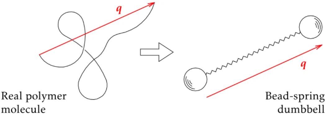
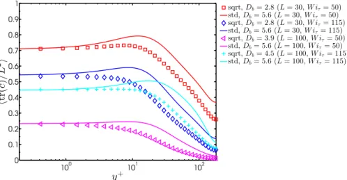
(25) Thèse de Ramon Silva Martins, Lille 1, 2016. List of Figures 1.1 Schematic representation of a real polymer molecule and its physical representation as a bead-spring dumbbell. The vector q is the end-to-end vector. . . . . . . . . . . . . . . . . . . . . . . . . . . . . . . . . . . . . . 2.1 Schematic representation of the channel geometry. . . . . . . . . . . . 3.1 Profiles of normalized components of the conformation tensor without artificial diffusion. (Dα = 0) . . . . . . . . . . . . . . . . . . . . . . . . . 3.2 Profiles of normalized components of the conformation tensor with the “a posteriori approach” for the artificial diffusion.(Dc = 10−6 ) . . . . . . 3.3 Profiles of normalized components of the conformation tensor with the “a posteriori approach” for the artificial diffusion.(Dα = 10−3 ) . . . . . 3.4 Profiles of normalized components of the conformation tensor with the “a priori approach” for the artificial diffusion. (Dc = 10−3 ) . . . . . . . 3.5 Time evolution of the bulk Reynolds number, Reh , for different formulations and initial conditions. . . . . . . . . . . . . . . . . . . . . . . . . 3.6 Profiles of the mean velocity and shear component of the Reynolds stress tensor in wall-units for several transformations of the conformation tensor and for different values of stress diffusion. (Reτ0 = 180, L = 30, W iτ0 = 50) . . . . . . . . . . . . . . . . . . . . . . . . . . . . . . . . . . 3.7 Profiles of the mean non-null components of the conformation tensor in wall-units by means of several transformations applied to it. (Reτ0 = 180, L = 30, W iτ0 = 50) . . . . . . . . . . . . . . . . . . . . . . . . . . . . . . 3.8 Mean trace of the conformation tensor in wall-units obtained with the standard (solid lines) and the square-root (open symbols) formulations for several elasticity levels. . . . . . . . . . . . . . . . . . . . . . . . . . 4.1 Schematic representation of the possible scenarios involving the rotation of a material element with respect to the eigenbasis of the strain-rate tensor. . . . . . . . . . . . . . . . . . . . . . . . . . . . . . . . . . . . . . 5.1 Contribution of each term in Eq. (5.6) (Q-criterion) at varied Reynolds numbers (Newtonian fluid): (a) Reτ0 = 180; (b) Reτ0 = 395; (c) Reτ0 = 590; and (d) Reτ0 = 1000 . . . . . . . . . . . . . . . . . . . . . . . . . . . . . 5.2 Contribution of each term in Eq. (5.5) (λ2 -criterion) at varied Reynolds numbers (Newtonian fluid): (a) Reτ0 = 180; (b) Reτ0 = 395; (c) Reτ0 = 590; and (d) Reτ0 = 1000; . . . . . . . . . . . . . . . . . . . . . . . . . . . . . 5.3 Contribution of each term in Eq. (5.6) (Q-criterion) at varied Reynolds numbers (viscoelastic fluid - L = 100 and W iτ0 = 115): (a) Reτ0 = 180; (b) Reτ0 = 395; (c) Reτ0 = 590; and (d) Reτ0 = 1000 . . . . . . . . . . . . . .. © 2016 Tous droits réservés.. 9 20 44 46 47 48 50. 53. 55. 56. 76. 86. 87. 88. lilliad.univ-lille.fr.

(26) Thèse de Ramon Silva Martins, Lille 1, 2016. xxvi. List of Figures. 5.4 Contribution of each term in Eq. (5.5) (λ2 -criterion) at varied Reynolds numbers (viscoelastic fluid - L = 100 and W iτ0 = 115): (a) Reτ0 = 180; (b) Reτ0 = 395; (c) Reτ0 = 590; and (d) Reτ0 = 1000; . . . . . . . . . . . . 5.5 Contribution of each term in Eq. (5.6) (Q-criterion) for varied elasticity levels at Reτ0 = 180: (a) L = 30 and W iτ0 = 50; (b) L = 30 and W iτ0 = 115; (c) L = 100 and W iτ0 = 50; and (d) L = 100 and W iτ0 = 115 . . . . . . . 5.6 Comparison of the contribution of each term in Eq. (5.6) (Q-criterion) between Newtonian and viscoelastic cases at Reτ0 = 1000. . . . . . . . 6.1 Contour of normalised criteria applied to the ABC flow. . . . . . . . . 6.2 Contour of normalised criteria applied to the flow in a 4:1 sudden contraction. . . . . . . . . . . . . . . . . . . . . . . . . . . . . . . . . . . . . 6.3 Iso-surfaces of Q = 2 (elliptic regions) from Reτ0 = 180 (first line) to Reτ0 = 1000 (last line). Newtonian cases are on the left-hand side and viscoelastic cases (L = 100 and W iτ0 = 115) are on the right-hand side. The displayed domain is restricted to 0 ≤ y ≤ 1 and 0 ≤ x ≤ 4π. Isosurfaces are coloured with the local intensity of u. . . . . . . . . . . . 6.4 Iso-surfaces of normalised criteria at the value of 0.25 (elliptic regions) at Reτ0 = 1000 for Newtonian fluid. The displayed domain is restricted to 0 ≤ y ≤ 1 and 0 ≤ x ≤ 4π. Iso-surfaces are coloured with the local intensity of u. . . . . . . . . . . . . . . . . . . . . . . . . . . . . . . . . 6.5 Iso-surfaces of normalised criteria at the value of 0.25 (elliptic regions) at Reτ0 = 1000 for viscoelastic fluid (L = 100 and W iτ0 = 115). The displayed domain is restricted to 0 ≤ y ≤ 1 and 0 ≤ x ≤ 4π. Iso-surfaces are coloured with the local intensity of u. . . . . . . . . . . . . . . . . . 6.6 Contours at z = 3π/4 of all normalised criteria applied to: (left column) Newtonian and (right column) viscoelastic (L = 100 and W iτ0 = 115) fluid at Reτ0 = 1000. The displayed domain is restricted to 0 ≤ y ≤ 1 and 0 ≤ x ≤ 4π. . . . . . . . . . . . . . . . . . . . . . . . . . . . . . . . . . . 6.7 Profiles of the plane-averaged non-objective criteria for Newtonian fluid at: (a) Reτ0 = 180; (b) Reτ0 = 395; (c) Reτ0 = 590; and (d) Reτ0 = 1000 . 6.8 Profiles of the plane-averaged objective criteria for Newtonian fluid at: (a) Reτ0 = 180; and (b) Reτ0 = 1000 . . . . . . . . . . . . . . . . . . . . . 6.9 Profiles of the plane-averaged objective ratios for Newtonian fluid at: (a) Reτ0 = 180; and (b) Reτ0 = 1000 . . . . . . . . . . . . . . . . . . . . . . . 6.10 Profiles of the plane-averaged criteria for two viscoelastic fluids (left column: L = 30 and W iτ0 = 50; right column: L = 100 and W iτ0 = 115) at Reτ0 = 1000: non-objective criteria in the first line ((a) and (b)); objective criteria in the second line ((c) and (d)); and objective ratios in the last line ((e) and (f)) . . . . . . . . . . . . . . . . . . . . . . . . . . . . . . . .. 90. 92 93 100 102. 104. 106. 107. 108 110 110 111. 113. C.1 Iso-contours of the normalized flow classification criteria applied to the ABC flow field: non-objective (first line) and objective (second line) versions of Q∗ -criterion, ∆∗ -criterion, λ∗2 -criterion and λ∗cr /λ∗ci -criterion. 144 C.2 Eigendirections of tensor D in the three planes for the ABC flow considD D ered. The ordering corresponds to the eigenvalues λD 145 1 ≥ λ2 ≥ λ3 . . . . C.3 Iso-contours of flow classifiers for the flow trough a 4:1 contraction: non-objective (left-hand side) and objective (right-hand side) versions of Q∗ -criterion, ∆∗ -criterion, λ∗2 -criterion and λ∗cr /λ∗ci -criterion. . . . . . . 146. © 2016 Tous droits réservés.. lilliad.univ-lille.fr.

(27) Thèse de Ramon Silva Martins, Lille 1, 2016. List of Figures. xxvii. C.4 Eigendirections of tensor D in the x − y plane for the 4:1 contraction flow. D D Again, the ordering corresponds to the eigenvalues λD 147 1 ≥ λ2 ≥ λ3 . . . D.1 Iso-contours of Q-criterion (Q = 1.5) for Newtonian (left column) and viscoelastic (right column) fluids at Reτ = 180, 395, 590 and 1000. . . D.2 Iso-contour for non-objective (a) and objective (d) versions of Q-criterion, and IR (b) and AR (c, e and f) criteria for Newtonian fluid at Reτ = 180. D.3 Contours of non-objective and objective criteria for Newtonian fluid at Reτ = 180. The xy-plane is located in the middle of the channel. . . . D.4 Contours of non-objective and objective criteria for viscoelastic fluid with L = 100 and W eτ = 115 at Reτ = 180. The xy-plane is located in the middle of the channel. . . . . . . . . . . . . . . . . . . . . . . . . . . . D.5 xz-plane averaged values of non-objective (left) and objective (right) criteria for Newtonian fluid at Reτ = 180. . . . . . . . . . . . . . . . . . D.6 xz-plane averaged values of non-objective (left) and objective (right) criteria for viscoelastic fluid with L = 100 and W eτ = 115 at Reτ = 180.. © 2016 Tous droits réservés.. 153 154 154. 155 156 156. lilliad.univ-lille.fr.

(28) Thèse de Ramon Silva Martins, Lille 1, 2016. xxviii. © 2016 Tous droits réservés.. List of Figures. lilliad.univ-lille.fr.

(29) Thèse de Ramon Silva Martins, Lille 1, 2016. General Introduction Motivation. The motion of fluids has always been a field of interest throughout history. Wind, vortices, buoyancy, convection, flight, navigation, pipe flow and many other aspects of fluid flow have been investigated until our days. With the formalisation of Fluid Mechanics, mainly after the contributions of Sir Isaac Newton, Poisson, Navier and Stokes (among many other remarkable scientists), the motion of many fluids could be predicted by the Navier-Stokes equation. This notorious equation describes the motion of low-molecular-weight fluids, notwithstanding several complex questions remain open and under investigation. Even more complex issues appear in the study of fluids whose motions can not be described by the Navier-Stokes equations. These fluids are known as non-Newtonian fluids. There are several examples of non-Newtonian fluids which are part of our daily lives by different ways, such as blood, toothpaste, printer ink, yogurt, butter, nail polish, etc. Among the non-Newtonian fluids, a variety of behaviours are possible, such as plasticity, viscoplasticity, thixotropy, elastoplasticity, elasticity, and viscoelasticity. We are particularly interested here in the flow of high-molecular-weight polymeric fluids, which present viscoelastic behaviour. “Visco” because they can somewhat resist shear as a viscous fluid. “Elastic” because they may respond to some degree as an elastic solid, deforming elastically and storing energy to, then, release it and recover partially their original shape. Viscoelastic fluids involve several “fascinating” (as qualified by Bird and Curtiss [1]) and sometimes also challenging phenomena. Bird, Armstrong, and Hassager [2, Chapter 3] showed and explained various effects of viscoelastic fluid flow, including rod-climbing, extrudate swell, the tubeless siphon, drag reduction in turbulent flow and vortex inhibition. The latter two will be somehow explored, in this thesis.. © 2016 Tous droits réservés.. lilliad.univ-lille.fr.

(30) Thèse de Ramon Silva Martins, Lille 1, 2016. 2. General Introduction. Polymer-induced drag reduction and its numerical simulation Over the last 20 years, the Direct Numerical Simulation (DNS) of viscoelastic fluid flows has been providing relevant information on the polymer-induced drag reduction phenomenon [3, 4]. After the pioneering DNS of Sureshkumar, Beris, and Handler [5], several numerical works have helped to enhance the knowledge about this phenomenon: Dimitropoulos and co-workers [6–9], De Angelis et al. [10], Min and co-workers [11, 12], Dubief et al. [13], Housiadas and co-workers [14–17], Dallas, Vassilicos, and Hewitt [18], Thais and co-workers [19–22] among others provided enriching data and discussions about the polymer-induced drag reduction. The polymer contribution to the Newtonian solvent is usually taken into account by means of a dumbbell model. Most of such models make use of a conformation tensor to describe polymer orientation [23]. By definition, the conformation tensor is Symmetric Positive Definite (SPD)1 . Nevertheless, numerical simulations of turbulent flows of viscoelastic fluids using highorder schemes usually face non-physical high-wavenumber instabilities (the so called Hadamard instabilities [24]) that cause the loss of the positive-definiteness of the conformation tensor. Consequently, the uncontrolled growth of the non-SPD points leads to non-physical results and the simulation usually break down after a few iterations. Several proposals to overcome this issue are available in the literature. One that has been largely used is the addition of an artificial stress diffusion [25] that brings an elliptical character to the hyperbolic evolution equation for the conformation tensor. Since diffusion has no physical meaning at the simulated scales (even for a DNS), the results obtained with this method will always be confronted to the question of how intrusive this additional term is with respect to the original model [26]. A less invasive alternative is to apply the artificial diffusion only to the domain points where the SPD condition is not fulfilled (e.g. [27]). Also, alternatives without any artificial term do exist. They are usually based on flux-limiter schemes to overcome the typical exponential growth on the field of the conformation tensor due to the steep gradients inherent to high-precision simulations of viscoelastic flows [18, 28–30]. More recent solutions propose transformations to be applied to the conformation tensor in order to enforce mathematically its positive-definiteness [31–34]. Some of these transformations however have not yet been tested in the context of turbulent viscoelastic shear flows exhibiting drag reduction, which brings us to part of the scope of this thesis. The polymer-induced drag reduction is known to change flow dynamics. One of the most evident changes in wall turbulence of viscoelastic fluid is the weakening and elongation of vortices [35]. Motivated by this changes, the evaluation of different 1A. © 2016 Tous droits réservés.. symmetric matrix M is SPD if z · M · zT > 0 for arbitrary (non-zero) z.. lilliad.univ-lille.fr.

(31) Thèse de Ramon Silva Martins, Lille 1, 2016. Vortex identification and flow classification in the context of turbulent viscoelastic fluid flows3 motions in the context of turbulent drag-reducing flows and the proper identification and interpretation is also being considered here.. Vortex identification and flow classification in the context of turbulent viscoelastic fluid flows The concept of a vortex is still cause for dissension within the scientific community. There is not a true consensus for the definition of a vortex. There are indeed several mathematical quantities available in the literature to identify a vortex. Some of them are very popular, such as the Q-criterion by Hunt, Wray, and Moin [36], ∆-criterion by Chong, Perry, and Cantwell [37], λ2 -criterion by Jeong and Hussain [38], λci -criterion by Zhou et al. [39]. Despite this hazy definition, what is consensual is that there are coherent rotating structures whose dynamics plays an important role in different transport phenomena, such as heat transfer, mixing, combustion, noise generation, aeroand hydrodynamic drag and other typically turbulent flows. Vortex identification and flow classification are closely linked, since, the ideas regarding vortex involve fluid rotation and one of the interests of flow classification is to separate, for instance, rotational and extensional regions of a flow. Besides the issue of defining a vortex, other discussions gravitating over properties that flow classification criteria must have also persist. One of them is whether a flow classification criterion should be invariant to arbitrary translating-rotating reference frame or to constant speed translations only. In other words, respectively, should a criterion enjoy Euclidean invariance or Galilean invariance only would be enough? Historically, the majority of flow classification criteria are Galilean invariant, but some authors claim that a solid criterion should be objective (or Euclidean frame indifferent), i.e. invariant to any possible transformation. In the context of viscoelastic flows, other questions arise: When applied to a viscoelastic fluid flow, should a flow classification criterion take into account rheological parameters or not? If one uses a criterion that was conceived for a Newtonian fluid in a viscoelastic fluid flow, how to interpret such results? Moreover, it is known that the polymer coil-stretch process affects vortex dynamics, but is it possible to go more into details? These are questions we will explore in this work.. Objectives The flow of viscoelastic fluids is a field in which numerous questions remain open due to the complexity of the phenomena. Among the open questions, we shall address the following in the present work:. © 2016 Tous droits réservés.. lilliad.univ-lille.fr.

(32) Thèse de Ramon Silva Martins, Lille 1, 2016. 4. General Introduction 1. Transformations for the conformation tensor in the numerical simulation of turbulent polymer-induced drag-reducing flows. The objective here is to evaluate the performance of more recent formulations for the conformations tensor that preserve the definite-positiveness of the conformation tensor. More precisely, the square-root [33] and the rootk kernel [34] transformations will be applied to turbulent channel flows. The need for maintaining (or not) an artificial stress diffusion in order to preserve numerical stability will also be assessed. 2. Vortex identification and flow classification in the context of turbulent viscoelastic flows and the role of objectivity. The goal here is to analyse the behaviour of objective versions of classic criteria available in the literature. The exercise will be conducted for several benchmark flows, such as the ABC flow, the abrupt contraction and the turbulent channel flow. Furthermore, recent flow classification criteria [40] which are naturally objective will be applied to the same flows. Finally, the contribution of polymers to the identification of vortices and its dynamics is investigated in the context of turbulent channel flow of viscoelastic fluids.. In both of these fronts, we will use the nnewt_solve algorithm developed by Thais et al. [19]. This code is a massively parallel scheme conceived to perform DNS of turbulent drag-reducing flows. It uses hybrid Fourier spectral and sixth-order compact finite differences schemes for spatial discretisation, and time marching can be up to fourthorder accurate. The parallelism is facilitated by a two-dimensional MPI Cartesian grid, together with OpenMP multi-threading. Regarding the first objective, the algorithm will be adapted to model the evolution equation for the transformation of the conformation tensor. The second objective involves mostly post-processing methodologies and theoretical discussions on the identification of vortices.. Organisation of the document This document is divided in two parts along the two objectives mentioned above. Part I consists on the application of transformations to the conformation tensor with the aim to avoid the loss of evolution in the simulation of turbulent wall-bounded viscoelastic fluid flows due to the lack of positive-definiteness of the conformation tensor. The need for maintaining or not an artificial stress diffusion is also assessed. Part II comprises theoretical discussions on the role of objectivity in flow classification and vortex identification. In a first moment, we discuss how the flow classification. © 2016 Tous droits réservés.. lilliad.univ-lille.fr.

(33) Thèse de Ramon Silva Martins, Lille 1, 2016. Organisation of the document. 5. criteria are impacted by the presence of polymers and how to take that into account when trying to make conclusions on the flow dynamics of viscoelastic fluids. Then, preliminary results for laminar and analytical flows are discussed. Finally, several criteria are applied to turbulent channel flows of both Newtonian and viscoelastic fluids. A portion of the results contained in this part is a compilation of the following works that have been published (journal paper and book chapter): • Ramon S. Martins, Anselmo S. Pereira, Gilmar Mompean, Laurent Thais and Roney L. Thompson. An objective perspective for classic flow classification criteria. Comptes Rendus Mécanique, 344, pp. 52–59, 2016. • Ramon S. Martins, Anselmo S. Pereira, Gilmar Mompean, Laurent Thais and Roney L. Thompson. On Objective and Non-objective Kinematic Flow Classification Criteria. In: Progress in Wall Turbulence 2: Understanding and Modelling. Eds. Michel Stanislas, Javier Jimenez, and Ivan Marusic. Cham: Springer International Publishing, 2016. pp. 419–428.. © 2016 Tous droits réservés.. lilliad.univ-lille.fr.

(34) Thèse de Ramon Silva Martins, Lille 1, 2016. 6. © 2016 Tous droits réservés.. General Introduction. lilliad.univ-lille.fr.

(35) Thèse de Ramon Silva Martins, Lille 1, 2016. Part I Evaluation of root-type transformations for the conformation tensor applied to turbulent channel flows of viscoelastic fluids. © 2016 Tous droits réservés.. lilliad.univ-lille.fr.


(37) Thèse de Ramon Silva Martins, Lille 1, 2016. Chapter. 1. Numerical simulation of viscoelastic fluid flow: State of the art The flow of viscoelastic fluids is fascinating because of the strange effects associated with them. The Newtonian fluid mechanics has been quite explored and reasonably explained. However, viscoelastic fluids behave differently. They exhibit non-linear and time dependent responses to deformation. Moreover, the stress is also anisotropic, i.e. it can present different behaviour according to the direction. These characteristics lead to instabilities that may appear in several geometries and at different flow regimes. From a numerical point of view, these effects are generally reproduced with the aid of viscoelastic fluid models. These models try to capture the essence of viscoelasticity and to simulate the effect of polymer solutions. Many options are now available in the literature, leading to several type of models: differential, integral, linear, nonlinear. Among these groups, there is an important class of models that approximates polymer molecules diluted in a Newtonian solvent as a set of beads and springs (see Fig. 1.1). q. q Real polymer molecule. Bead-spring dumbbell. Figure 1.1 – Schematic representation of a real polymer molecule and its physical. representation as a bead-spring dumbbell. The vector q is the end-to-end vector. The beads represent very small polymer monomers while the springs connecting them act like a restoring force that virtually represent the tendency of polymer chains. © 2016 Tous droits réservés.. lilliad.univ-lille.fr.

(38) Thèse de Ramon Silva Martins, Lille 1, 2016. 10. CHAPTER 1. Numerical simulation of viscoelastic fluid flow: State of the art. to coil. These models are also referred to as dumbbell models. Hookean (linear) springs present infinite extensibility and, even so, can reasonably reproduce lots of viscoelastic phenomena. One of the most used Hookean dumbbell models is the Oldroyd-B model [23]. On the other hand, limiting the polymer stretch leads to an important class of models known as Finitely Extensible Nonlinear Elastic (FENE) models [23]. Besides the more realist physical foundation behind these models (when compared to linear elastic models), they are able to better approach combinations of a given polymer-solvent by varying its parameters. One drawback of the FENE model is that it does not have a closure that allows its implementation for numerical calculations on general transport phenomena. In an effort to obtain results with such a promising methodology, several closures have been proposed, as, for instance, FENE-P [41], FENE-CR [42], FENE-L and FENE-LS [43, 44], FENE-CD [45], FENE-DT [46], FENE-QE [47]. Usually, the interesting viscoelastic effects are time-dependent and, some of them, get more intense with increasing elasticity. When performing simulations of unsteady viscoelastic fluid flows, however, it is quite common to find limitations due to numerical instabilities.. 1.1. The conformation tensor and its properties. Dumbbell models are usually based on a tensor that carries information about the configuration of each individual polymer molecule. This tensor is usually named conformation tensor and is formed by the components of the end-to-end vector that connects the polymer chain ends [23]. Because of its physical meaning and mathematical representation, the conformation tensor is symmetric and positive definite (SPD) and must remain so. In particular, in the FENE-P model, the conformation tensor receives another constraint due to the approximation proposed by Peterlin [41]. This approximative closure consists on a pre-averaging in space for the end-to-end vector. Consequently, the trace of the conformation is then bounded by the square of the maximum chain extensibility imposed by the pre-averaging. Vaithianathan and Collins [26] point out three issues associated to the conformation tensor in numerical simulations. • Positiveness (or positive-definiteness) of the conformation tensor. Negative eigenvalues are equivalent to locally negative viscosity. Thus, the loss of positive-definiteness gives rise to instabilities that may lead to non-physical results or even numerical divergence. • Boundedness of the conformation tensor.. © 2016 Tous droits réservés.. lilliad.univ-lille.fr.

(39) Thèse de Ramon Silva Martins, Lille 1, 2016. 1.2. High Weissenberg Number Problem and loss of positiveness in viscoelastic flows11 For models that consider a finite extensibility to the polymer chain (such as the FENE-P model), special attention should be given to the trace of the conformation tensor, which indicates how stretched the polymer molecules are. For instance, in the FENE-P model, the trace is bounded by the theoretical upper value of the chain extensibility squared. All the same, highly extensional flows may give rise to numerical errors due to overextension of the conformation tensor. When this happens, the restoring force changes sign, leading to divergence. The authors comment that solving the equations implicitly may partially alleviate this, but the price is a much slower convergence rate. • Lack of a dissipation mechanism. If, for any reason, steep gradients are generated in the conformation tensor, the polymer stress divergence might increase without bound. The authors state that, physically, a molecular mechanism is expected to truncate this growth, but no diffusion term is included in most used models. These three points are challenges for the scientific community involved in the simulation of viscoelastic flows. Notably, the third issue concerns turbulent flows, in which sharp gradients are more common. In an effort to better understand how the properties of the conformation tensor affect the simulation of viscoelastic flows, the literature review presented below is split in three sections. Each section contains the main effects observed under specific conditions, the limitations of their numerical simulations and the main solutions available. The first section is dedicated to laminar flows, the second section presents the special case of elastic turbulence, and the third section discusses (inertial) turbulent phenomena, such as drag reduction, on which our attention is focused here.. 1.2. High Weissenberg Number Problem and loss of positiveness in viscoelastic flows. Simulating viscoelastic flows in complex geometries has been a challenge to the scientific community. According to Keunings [48], “ever since the early attempts of the mid 1970’s, researchers have repeatedly met with an outstanding problem, namely the failure of their numerical schemes to provide solutions beyond some critical value of the Weissenberg number [. . . ]”. This has been often referred to as the High Weissenberg Number Problem (HWNP). The critical Weissenberg number depends on the geometry and on the model (constitutive equation) used for the polymer solution. In order to understand the HWNP, the problem has been addressed from different fronts. Basically, mathematical and numerical explanations were sought.. © 2016 Tous droits réservés.. lilliad.univ-lille.fr.

(40) Thèse de Ramon Silva Martins, Lille 1, 2016. 12. CHAPTER 1. Numerical simulation of viscoelastic fluid flow: State of the art. Rutkevich [49–52] firstly explored the evolutionary conditions of viscoelastic flows using Maxwellian fluids. In the work of Joseph, Renardy, and Saut [53], the change of (mathematical) type of the system of equations was investigated and the concept of Hadamard instability [24] in this context was introduced. The authors claim that small instabilities caused by ill-posed initial(-boundary) value problems may lead to oscillations that grow exponentially. Physically, it may warn about instabilities, but, in the context of numerical simulation, this leads to divergence [54]. Following that, several fluid models and flows were explored [24, 55–59]. In the late 1980’s some first workarounds were proposed. The concomitant advances in parallel computation and numerical methods lead to the further evolution of more successful simulations that were able to explore slightly higher elasticity values and more complex flows with more accuracy and stability. We present in the following the main methods that contributed to such evolution.. 1.2.1. Some remedies available. The first strategies consisted of manipulating the constitutive equation so that their elliptic character could be somehow split from the hyperbolic one. This leads to numerical stability, mainly because of the smoothing character coming with ellipticity. This was the case, for instance, for the following schemes: Explicitly Elliptic Momentum Equation (EEME) [60], Elastic-Viscous Stress Splitting (EVSS) [61], and Adaptive Viscoelastic Stress Splitting (AVSS) [62]. Even though these solutions were the first proposed to stabilise the simulation of viscoelastic fluid flows, they are still quite used nowadays, sometimes combined with more recent methods. Alves, Oliveira, and Pinho [63] came up with a high resolution scheme that limits the flux of advection terms with good iterative convergence. The so called Convergent and Universally Bounded Interpolation Scheme for the Treatment of Advection (CUBISTA) was tested in a code based on finite-volume, for Newtonian flows over a backwardfacing step, and viscoelastic flows past a cylinder and in a sudden contraction. For the viscoelastic flows, the CUBISTA scheme was also used for the advection term in the constitutive equation, leading to better stability and accuracy. By using a unique decomposition to the velocity gradient, Fattal and Kupferman [31] reported a new logarithmic transformation for the conformation tensor. The authors were inspired by the idea of smoothing the steep gradients that arise in the field of the conformation tensor. They applied their methodology to the lid-driven cavity flow of a FENE-CR [42] fluid without the need of an artificial stress diffusion. Using a finite difference framework, they stated that their scheme remains stable at moderately high Weissenberg numbers. Later, the authors presented more detailed results with an Oldroyd-B fluid [32] and affirm that for sufficiently high Weissenberg numbers, strong. © 2016 Tous droits réservés.. lilliad.univ-lille.fr.

(41) Thèse de Ramon Silva Martins, Lille 1, 2016. 1.2. High Weissenberg Number Problem and loss of positiveness in viscoelastic flows13 oscillations lead to divergence. More recently, Balci et al. [33] showed that there is also a unique square-root transformation for the conformation tensor that can guarantee its positive-definiteness. The authors presented the formulation for both Oldoryd-B and FENE-P fluids. However, they performed simulations of Stokesian flows using Oldroyd-B fluids without any artificial stress diffusion. Higher Weissenberg numbers could be achieved with improved stability and accuracy, although limitations were still found with increasing elasticity. The authors highlighted the easy implementation and the low CPU requirements of their formulation compared to logarithmic transformation. Their statement is based on the fact that their method does not require the calculation of eigenvalues and eigenvectors of the conformation tensor at every time step. Afonso, Pinho, and Alves [34] gathered the decomposition of the velocity gradient by Fattal and Kupferman [31] and the idea of applying transformations to the conformation tensor to present a generic framework for a large group of matrix transformations. The so-called kernel transformation has shown to recover the log- and square-rootconformation formulations. The method was tested for a confined cylinder flow of an Oldroyd-B fluid for various logarithm-based and root-based models (among others). They concluded that the kernel transformation can be used to gain numerical stability, but the best choice of kernel function depends on its capacity of smoothing gradients in the conformation field and still preserve its positiveness. It is important to remark that the square-root formulation deriving from the kernel transformation differs from the originally proposed by Balci et al. [33]. The main difference is that, in the kernel transformation framework, the calculation of eigenvalues and eigenvectors of the conformation tensor is required in the whole domain at every time step. The alternatives cited above have been tested in different contexts in laminar viscoelastic flows. Among many others, one may cite the use of EVSS and AVSS to simulate extrudate swell [64], EVSS to simulate 180° bent planar channel and in a 4:1 planar contraction [65], lid-driven cavity, flow past a cylinder, 4:1 contraction using the square-root and the logarithm conformations with the CUBISTA scheme [66], the log-conformation to simulate a lid-driven cavity [67] and the flow past a cylinder [68], the square-root transformation combined with the CUBISTA scheme to solve the lid-driven cavity flow, the flow around a confined cylinder, the cross-slot flow and the impacting drop free surface problem [69], a combination of the kernel conformation with CUBISTA scheme to simulate the Poiseuille flow in a channel, the lid-driven cavity flow and the extrudate-swell free surface flow with Oldroyd-B fluid [70], and, more recently, the Weissenberg effect [71] using the kernel-conformation.. © 2016 Tous droits réservés.. lilliad.univ-lille.fr.

(42) Thèse de Ramon Silva Martins, Lille 1, 2016. 14. 1.3. CHAPTER 1. Numerical simulation of viscoelastic fluid flow: State of the art. Elastic turbulence: nor simply laminar, neither merely turbulent. The flow of polymer solutions at vanishing Reynolds number and high level of elasticity indicates chaotic fluctuations in time and space, similar to those observed in (inertial) turbulent flows. It is known now that this phenomenon is purely elastic and it is usually referred to as elastic turbulence [72]. Experiments suggest that the onset of elastic turbulence is associated to curvilinear streamlines. Therefore, most of successful numerical simulations of this phenomenon so far have been carried out using curvilinear geometries or imposing forces to the flow field that produces circular motion. In the curvilinear geometry context, Thomas, Sureshkumar, and Khomami [73] performed DNS of 3D time-dependent Taylor-Couette flows of a FENE-P fluid. The authors found instabilities of elastic origin demonstrating spatial and time variation patterns. For these simulations, the authors adapted a fully spectral algorithm previously used for turbulent channel flows [5] that uses artificial diffusion to avoid the loss of positiveness and ensure stability (see the next section for more information on the use of artificial diffusion). More recently, Feng-Chen et al. [74] simulated curvilinear channel flow driven by pressure gradient. The authors used a Giesekus [75] model also with the addition of artificial diffusion (as proposed by [25]) to avoid steep oscillations and undershoot/overshoot. They present a brief and preliminary explanation of intermittent energy pumping in the flow. Concerning wall-free flows with an imposed curvilinear force term, Berti and coauthors [76, 77] conducted DNS of Kolmogorov flows using the Oldroyd-B model with the Cholesky decomposition proposed by Vaithianathan and Collins [26] to guarantee the maintenance of positiveness for the conformation tensor. Stationary states transits to a chaotic state when properly excited over a critical Weissenberg number. The power spectrum of velocity fluctuations in chaotic state is found to be close to experimental results. Thomases and Shelley [78] performed simulations of 2D periodic Stokesian flows using the Oldroyd-B model in a pseudospectral code. They found two transitions: one being steady and asymmetric and the other being oscillatory. Results using a classic straight channel flow are also available. On one hand, HongNa et al. [79] added a sinusoidal force term to both the momentum equation and the Giesekus constitutive equation of their DNS to excite the flow, usually stable. The authors conclude that large shear rates are important to elastic turbulence, because, at the regions where they occur, strong stretching and more intense vortical activity are observed. On the other hand, Samanta et al. [80] introduced the concept of elasto-inertial turbulence. They performed pipe flow experiments and DNS of channel flows using the FENE-P model with local artificial diffusion (see the next section for. © 2016 Tous droits réservés.. lilliad.univ-lille.fr.

(43) Thèse de Ramon Silva Martins, Lille 1, 2016. 1.4. Turbulent viscoelastic flows: the drag reduction phenomenon. 15. further information about local artificial diffusion). The authors stress that their results contain a non-negligible amount of inertia, but, still, it seems to be related to elastic turbulence. They found that the transition point to turbulence is delayed when polymer solutions are compared to their relative Newtonian cases. Moreover, they noticed that elastic instabilities that appear at the regions of large shear rate lead to friction factors comparable to the Maximum Drag Reduction (MDR) regime (further information on MDR is available in the next section). In a very recent paper, Ray and Vincenzi [81] used a shell model that imitates the Fourier modes of the velocity field and of the polymer configuration field for a viscoelastic fluid flow without the information on the spatial structure of these fields. The resulting formulation is like a reduced low-dimensional version of the FENE model [23]. The authors verify the transitional and the chaotic states of elastic turbulence for different Weissenberg numbers and polymer concentrations, concluding that these two parameters show similar influence on the transition to elastic turbulence. Moreover, they claim that the physical mechanisms that lead to elastic turbulence do not depend on the boundary conditions, nor on the mean flow. In short, even though elastic turbulence is a recent discovery and the methodology for its numerical simulation is still being discussed, some important results are already available. Regarding the issues related to the conformation tensor, since elastic turbulence has a lot in common with inertial turbulence, its simulation undergoes the same limitations. To avoid that, artificial diffusion is mostly used. This and other solutions to overcome the numerical instabilities associated to turbulent viscoelastic flows are presented in the next section.. 1.4. Turbulent viscoelastic flows: the drag reduction phenomenon. The dilution of very small amounts of high-molecular-weight polymers in a Newtonian fluid may lead to a diminution of pressure drop in turbulent flows. This phenomenon, known as polymer-induced drag reduction, has been explored since its first observations in the 1930’s, by Forrest and Grierson [82] and in the 1940’s by Toms [83] and Mysels [84]. Almost 80 years later, even though many advances have been made, a complete and consensual theory on the mechanism of drag reduction is still being sought. Virk, Mickley, and Smith [85] provided a systematic experimental analysis of the polymer-induced drag reduction phenomenon in turbulent pipe flows. The author investigated the onset of the phenomenon and found an asymptotic upper limit usually referred to as Maximum Drag Reduction MDR. The sensitivity of the phenomenon and its features were tested for varying polymer’s concentration, molecular weight, and. © 2016 Tous droits réservés.. lilliad.univ-lille.fr.

(44) Thèse de Ramon Silva Martins, Lille 1, 2016. 16. CHAPTER 1. Numerical simulation of viscoelastic fluid flow: State of the art. Reynolds number. Two major theories try to explain the polymer-induced drag reduction phenomenon. Lumley [86] and Seyer and Metzner [87] proposed independently that the polymers chains are stretched due to the turbulent flow outside the viscous sublayer, leading to an increase of the effective viscosity in the turbulent region. The thickness of the viscous sublayer and of the buffer layer is therefore increased, reducing the velocity gradient near the wall, and, consequently, the drag. Because its explanation is based on the increase of effective viscosity, this theory is mostly known as viscous theory. Tabor and de Gennes [88] came up with the idea that, due to its elastic properties, polymers store part of the turbulent energy in the buffer layer. When the elastic (stored) energy becomes comparable to the turbulent energy, the energy cascade is affected. Since the length of elastic scales associated to this action is larger than the Kolmogorov scale, the buffer layer is thickened and drag is reduced. This proposed mechanism is known as elastic theory. The direct numerical simulation (DNS) of this phenomenon has been helping to clarify some physical issues related to it. DNS provides precious information about the interaction between polymer chains and the flow field which lead to new viewpoints of the phenomenon that sometimes could not be obtained experimentally. By performing the direct numerical simulation of turbulent pipe flows and using a constitutive equation that relates the elongational viscosity to the second and third invariants of the rate-of-strain tensor, Den Toonder, Nieuwstadt, and Kuiken [89] were able to conclude that not only the effect of polymer stretch is relevant to the drag reduction mechanism, but the polymer compression (or coiling) motion is important as well. Orlandi [90] simulated a channel flow using a constitutive equation for which the elongational viscosity is a function of the rate of the strain rate to the rotation rate. The author reproduced qualitative results of the polymer drag reduction phenomenon for a minimal channel. The results were obtained using a pseudospectral algorithm (Chebishev polynomials + Fourier expansions). Concerning time integration, the referred algorithm treated viscous terms with implicit schemes, while nonlinear terms were treated explicitly. Beris and Sureshkumar [91] presented a fully spectral simulations of a threedimensional turbulent channel flow using various viscoelastic fluids: the upper convected Maxwell [92], the Oldroyd-B [23] and the Chilcott-Rallison (FENE-CR) [42] models. They used a mixed explicit/implicit time-integration algorithm. The authors also investigated the effect of an artificial stress diffusion term on the stability of turbulent channel flows using the Oldroyd-B model [25]. This technique is known as Global Artificial Diffusion (GAD). They concluded that with an appropriate stress diffusion, the numerical stability is considerably enhanced without significant changes in the flow. © 2016 Tous droits réservés.. lilliad.univ-lille.fr.

(45) Thèse de Ramon Silva Martins, Lille 1, 2016. 1.4. Turbulent viscoelastic flows: the drag reduction phenomenon. 17. characteristics. Later, Sureshkumar, Beris, and Handler [5] conducted direct numerical simulations of turbulent channel flows with the FENE-P model [23]. Very good qualitative agreement was observed when comparing their results to the tendencies of statistics and dynamics of experimental drag reduction results. However, even if this solution is largely used by Beris and co-workers [5, 14–17, 93] and other groups [6, 10, 19, 20, 94], it brings a non-physical term into the equation, which must be adjusted to be as small as possible. In a first effort to find less intrusive approaches, Min and co-workers [11, 12, 27] introduced the idea of Local Artificial Diffusion (LAD). Instead of considering the artificial stress diffusion globally, i.e. to the whole domain (actually, with the exception of boundary points), they applied the artificial diffusion locally, only at locations where the constraints for the conformation tensor were being violated. This methodology has been proved to also provide stability and physical results in accordance with the literature trends. More precisely, their results using LAD in a third-order compact upwind difference scheme led to more drag reduction than those with GAD. The authors claim that the dissipative error caused by local artificial diffusion term is negligible since the calculation points in which such term is needed change with time marching and do not pass 0.5% of the total grid points of the tested cases. The same method has been successfully used by Dubief and co-authors in [13, 95]. Two decompositions that preserve both positiveness and boundedness (if the model predicts so) of the conformation tensor have been proposed by Vaithianathan and Collins [26]. One of them consists of applying an eigendecomposition to the conformation tensor and evolving its eigenvalues and eigenvectors separately. The other one is based on a Cholesky decomposition to a mapped conformation tensor along with a logarithm transformation applied to the decomposed tensor. These two methods were applied to the FENE-P model and tested for isotropic turbulent flows. Comparisons with the standard conformation formulation with and without artificial diffusion were also conducted. By performing uncoupled simulations (in which the polymer field does not affect the velocity field), the authors showed that both proposed decompositions eliminate the occurrence of negative eigenvalues of the conformation tensor. With the standard formulation with artificial diffusion, the frequency of their occurrence is only attenuated, meaning that negative eigenvalues are still occurring. In a later publication by Vaithianathan et al. [28], it was discussed that the numerical scheme used in [26] did preserve the positiveness of the conformation tensor, but not its conservation. They argued that, in fact, regarding spectral and high-order compact schemes, artificial diffusion seems to be the solution to discontinuities in the field of the conformation tensor that causes undershoots or overshoots in the conformation tensor, which may lead to negative eigenvalues. They claim however that capturing the polymer strength around discontinuities is essential to calculate. © 2016 Tous droits réservés.. lilliad.univ-lille.fr.

(46) Thèse de Ramon Silva Martins, Lille 1, 2016. 18. CHAPTER 1. Numerical simulation of viscoelastic fluid flow: State of the art. turbulent flows of polymer solutions. They assert that spectral and high-order compact schemes are not naturally appropriate to solve hyperbolic equations. Moreover, possible alternatives are somehow difficult to deal with. Thus, they opted for a second-order finite-difference bound-preserving scheme which was originally conceived to guarantee the positiveness of scalar field based on flux limiters, but that they extended to tensor fields. The authors reported unconditionally stable results of the new algorithm for homogeneous turbulence. The effect of artificial stress diffusion was tested and resulted in a diminution of the drag reduction percentage of 10-15% and underestimation of polymer stretching. Yu and Kawaguchi [29] introduced a high-resolution flux-limiter algorithm with which they were able to simulate drag-reducing channel flows using the Giesekus model without any artificial diffusion. The effect of artificial diffusion was assessed with another algorithm of their own. They reported higher drag reduction regimes (percentages) with their new algorithm. Beris and Housiadas [96] argue that the stress diffusivity used by Yu and Kawaguchi [29] is higher than usual for spectral methods. Moreover, if one is interested on the mechanisms of polymer stretching and flow dynamics in various time and spatial scales, spectral methods are very suitable. By adapting the periodic algorithm of Vaithianathan et al. [28] to wall-bounded flows, Dallas, Vassilicos, and Hewitt [18] performed drag-reducing channel flows without any artificial assumption for FENE-P fluids. At the same time, Housiadas, Wang, and Beris [17] combined the log-conformation together with a mapping scheme that preserves the boundedness of the conformation tensor. Their algorithm is almost fully spectral, the only exception being a second-order finite-difference multigrid scheme to solve the stress diffusion term added to the constitutive equation. It is worth noting that the simulation of homogeneous isotropic turbulence of viscoelastic fluids also requires special attention on the loss of evolution, but they will not be concerned here. Just to cite a few examples of applications in this context, De Angelis et al. [97] used the artificial diffusion [5, 25], Perlekar, Mitra, and Pandit [98] made use of the Cholesky decompostion proposed by [26], and Cai, Li, and Zhang [99] applied the eigendecomposition in [28].. © 2016 Tous droits réservés.. lilliad.univ-lille.fr.

(47) Thèse de Ramon Silva Martins, Lille 1, 2016. Chapter. 2. Mathematical modelling and numerical method The introduction in the previous chapter substantiates that the simulation of turbulent viscoelastic flows is not trivial, since it involves numerical instabilities coming from the hyperbolic nature of the constitutive equations that potentially grow due to the lack of a dissipation mechanism in the model. Basically, two options should be weighted to overcome this: either one privileges the spatial accuracy of spectral and high-order compact schemes and use an artificial stress diffusion that smooths the shocks in the conformation tensor, or the somewhat intrusive artificial diffusion is avoided, by using flux limiter schemes paying the price of lower order accuracy (typically second order). In this chapter, the mathematical models and numerical methods are presented. The DNS code used here considered originally the standard conformation tensor formulation for FENE-P fluids with the inclusion of a global artificial stress diffusion to avoid the breakdown due to the loss of positive-definiteness. The minimum diffusivity coefficient was properly adjusted to provide numerical stability. In general, with this approach, the amount of grid points in which the conformation tensor presents non-positive eigenvalues corresponds to at most 1% of the total number of grid points. The formulations for the square-root and the kernel transformations are presented and the need to maintain or not the artificial stress diffusivity for these formulations is also evaluated.. 2.1. Basic equations. For the three-dimensional channel flow considered here, the position vector x∗ reads x∗ = (x1∗ , x2∗ , x3∗ ) = (x∗ , y ∗ , z∗ ), where x∗ is the stream-wise direction, y ∗ is the wall-normal direction, and z∗ is the span-wise direction1 . The channel has dimensions (L∗x , L∗y , L∗z ), 1A. © 2016 Tous droits réservés.. superscript asterisk is used to denote dimensional variables.. lilliad.univ-lille.fr.

(48) Thèse de Ramon Silva Martins, Lille 1, 2016. 20. CHAPTER 2. Mathematical modelling and numerical method. corresponding to the same respective directions above. Figure 2.1 provides a schematic representation of the geometry.. Figure 2.1 – Schematic representation of the channel geometry.. The flow satisfies the mass conservation equation (or continuity equation). Assuming the fluid to be incompressible, this reads ∇∗ · u∗ = 0. (2.1). .. The generalised form of the Navier-Stokes equations (the balance of momentum) is Du∗ ∂u∗ 1 1 = ∗ + u∗ · ∇∗ u∗ = − ∇∗ p∗ + ∇∗ · T ∗ ∗ Dt ∂t ρ ρ. ,. (2.2). where u∗ is the velocity vector with entries (u1∗ , u2∗ , u3∗ ) = (u ∗ , v ∗ , w∗ ), corresponding respectively to the directions (x∗ , y ∗ , z∗ ). The dimensional time is represented by t ∗ . The velocity gradient ∇∗ u∗ has entries ∇∗ uij∗ ei ⊗ ej = ∂uj∗ /∂xi∗ ei ⊗ ej . It is important to introduce also the transpose of the velocity gradient2 , L∗ = ∇∗ u∗T . The pressure is represented here by p∗ and ρ∗ stands for the fluid density. The symbol ∇∗ () corresponds to the gradient operator, while ∇∗ · () stands for the divergence operator. The material derivative is indicated by D()/Dt. The boundary conditions for the velocity field are: periodicity in the homogeneous directions (stream-wise, x∗ , and span-wise, z∗ ) and no-slip wall condition at the walls. In this generalised representation of the Navier-Stokes equations, the stress tensor T ∗ may be split into two parts, T ∗ = TN ∗ + TP ∗. ,. (2.3). TN ∗ = 2µ∗0 βD ∗. ,. (2.4). in which. 2 The. expression velocity gradient is used interchangeably for ∇∗ u∗ or L∗ and for the non-dimensional. ∇u or L.. © 2016 Tous droits réservés.. lilliad.univ-lille.fr.

(49) Thèse de Ramon Silva Martins, Lille 1, 2016. 2.1. Basic equations. 21. takes into account the Newtonian contribution, while TP ∗ represents the polymeric contribution. In Eq. (2.4), β is the ratio of the solvent dynamic viscosity, µ∗S , to the total zero-shear-rate solution dynamic viscosity, µ∗0 = µ∗S + µ∗p0 (where µ∗p0 is the polymeric zero-shear-rate dynamic viscosity), and D ∗ is the rate-of-strain tensor, defined as the symmetric part of the velocity gradient, D ∗ = (L∗ + L∗T )/2. The value of β works as an indicator for the polymer concentration, so that the limit of β = 1 yields the Newtonian case. The contribution, TP ∗ , due to the presence of polymers is defined by the constitutive equation chosen to model it and is proportional to 1 − β (see Subsection 2.1.1 below). The equations are made non-dimensional using the bulk velocity Ub∗ as a velocity scale and the channel half width h∗ (= L∗y /2) as a length scale. The time scale thus becomes h∗ /Ub∗ . The non-dimensional variables and operators are u=. u∗ Ub∗. ,. t=. t ∗ Ub∗ h∗. ,. x=. x∗ h∗. p=. ,. p∗ ρ∗ Ub∗ 2. ,. ∇ = h∗ ∇∗. ,. (2.5). The non-dimensional form of Eqs. (2.1) and (2.2) is ∇·u = 0. (2.6). ,. β ∂u 1 + u · ∇u = −∇p + ∆u + ∇·Ξ . ∂t Reh Reh. (2.7). In Eq. (2.7) above, the bulk Reynolds number, Reh , is based on the channel half gap, h, and calculated as Reh = h∗ Ub∗ /ν0∗ (ν0∗ being the total zero-shear-rate kinematic viscosity defined as µ∗0 /ρ∗ ). The term Ξ is the extra-stress tensor which contains non-dimensional the polymer contribution (TP ∗ ) and reads Ξ=. h∗ T ∗ µ∗0 Ub∗ P. .. (2.8). In order to close the problem formed by the set of Eqs. (2.6) and (2.7) we need a model for Ξ which is given by the constitutive equation.. 2.1.1. Constitutive equations: modelling polymer solutions. In the present work, the FENE model with the closure proposed by Peterlin [41] (known as the FENE-P model [23]) was chosen to account for the polymeric stress, Ξ. This model has been largely used in the context of turbulent drag-reducing flows due to its relatively simple second-order closure. The FENE-P model requires the solution of the phase-averaged configuration tensor, c, usually named conformation tensor. The non-dimensional conformation tensor is. © 2016 Tous droits réservés.. lilliad.univ-lille.fr.