Reliable robot localization: a constraint programming approach over dynamical systems

HAL Id: tel-03010085

https://hal.archives-ouvertes.fr/tel-03010085

HAL is a multi-disciplinary open access

archive for the deposit and dissemination of sci-entific research documents, whether they are pub-lished or not. The documents may come from teaching and research institutions in France or abroad, or from public or private research centers.

L’archive ouverte pluridisciplinaire HAL, est destinée au dépôt et à la diffusion de documents scientifiques de niveau recherche, publiés ou non, émanant des établissements d’enseignement et de recherche français ou étrangers, des laboratoires publics ou privés.

Reliable robot localization: a constraint programming

approach over dynamical systems

Simon Rohou

To cite this version:

Simon Rohou. Reliable robot localization: a constraint programming approach over dynamical sys-tems. Robotics [cs.RO]. Lab-STICC; UBO Brest; ENSTA Bretagne; University of Sheffield, 2017. English. �tel-03010085�

Reliable robot localization:

a constraint programming approach

over dynamical systems

under the seal of the Brittany-Loire University to obtain the title of

DOCTOR OF THE UNIVERSITY OF WESTERN BRITTANY

Branch: Robotics

Doctoral School Maths-STIC

presented by

Simon Rohou

Prepared at the ENSTA Bretagne (Lab-STICC, FR) and at the University of Sheffield (UK)

Thesis defended on 11th December 2017

before the jury composed of:

- Hisham Abou-Kandil, president of the jury

Professor, ´Ecole Normale Sup´erieure, Cachan, FR

- Philippe Bonnifait, rapporteur

Professor, Heudiasyc, Compi`egne, FR

- Gilles Trombettoni, rapporteur

Professor, LIRMM, Montpellier, FR

- Gilles Chabert, reviewer

Associate Professor, LS2N, Nantes, FR

- Benoit Zerr, reviewer

Professor, Lab-STICC, Brest, FR

- Luc Jaulin, thesis co-supervisor

Professor, Lab-STICC, Brest, FR

- Lyudmila Mihaylova, thesis co-supervisor

Professor, the University of Sheffield, UK

- Fabrice Le Bars, thesis co-supervisor

Reliable robot localization:

a constraint programming approach

over dynamical systems

Simon Rohou

Acknowledgments

Que de chemin parcouru pendant ces trois ann´ees de th`ese... et voila d´ej`a le moment de poser un point final sur la synth`ese de ce doctorat. Je ne saurais finir ce travail

sans avoir une pens´ee pour les nombreuses personnes qui ont crois´e mon chemin

tout au long de cette aventure.

Je remercie en premier lieu mes encadrants pour l’´energie d´eploy´ee au cours de

ces trois ann´ees. First, a special thank to Pr. Lyudmila Mihaylova and Pr. Sandor

M. Veres for their hospitality in Sheffield and the discussions around this work, making this Franco-British collaboration a memorable experience. J’adresse ma sinc`ere reconnaissance `a Fabrice Le Bars pour sa grande disponibilit´e, son soutien technique et ses nombreux retours sur ce travail. Enfin, je remercie chaleureusement

Luc Jaulin pour son encadrement exceptionnel, ses «Alors cette th`ese ?» quotidiens

et la confiance qu’il m’a accord´e, depuis mes premiers jours de th`ese jusqu’`a

l’affrontement final dans l’ar`ene de la soutenance.

Aussi je souhaite naturellement remercier les membres de mon jury pour le temps consacr´e `a la lecture de ce manuscrit et leur pr´esence lors de la soutenance.

En particulier, merci `a Philippe Bonnifait pour son enthousiasme constructif et

l’int´erˆet port´e aux applications de ces travaux en robotique, ainsi qu’`a Gilles

Trombettoni pour son optimisme constant sur ces probl´ematiques de tubes. Je

remercie ´egalement Hisham Abou-Kandil d’avoir pr´esid´e ce jury ainsi que Gilles

Chabert et Benoit Zerr qui ont endoss´e les rˆoles d’examinateurs. J’ai ´et´e honor´e

d’avoir un jury si h´et´erog`ene : vos nombreuses remarques et observations me

donnent d´ej`a du grain `a moudre pour le futur.

Mes pens´ees s’adressent ´evidemment `a mes amis doctorants et chercheurs de

tous horizons qui ont contribu´e, chacun `a leur mani`ere, `a un environnement de

travail sain et captivant dans ce bout du monde brestois. Je pense bien entendu `a

mes deux co-bureaux du M025, si souvent surnomm´e La conciergerie : Thomas

Le M´ezo, pour les innombrables bavardages, les coups de main jusqu’au lac de

Polytechnique et Piombino, et son dynamisme bien souvent trop d´ebordant qui

aura profit´e `a tant de projets. Merci ´egalement `a Benoˆıt Desrochers, alias Benoid, pour sa g´en´erosit´e, son amiti´e et tout ce temps pass´e `a traiter les donn´ees de

Daurade.

Et comment oublier les d´ebriefings du vendredi soir en compagnie des roboticiens.

Merci `a Benoit Zerr, alias Benoiz, pour son humour quotidien, sa bonne humeur,

ou caf´eique. Je tire mon chapeau `a Michel Legris, qui communique si facilement

sa grande passion pour les sciences : un v´eritable plaisir que de d´ecouvrir toutes

ces anecdotes captivantes, de discuter de probl`emes sordides ou de d´ebattre de

l’int´erˆet d’ˆetre pessimiste. Merci ´egalement `a Rod´eric Moiti´e pour sa gentillesse et

son amiti´e, ses coups de main et sa passion pour la photographie. J’esp`ere que nous

aurons d’autres occasions de sortir les 70D pour capturer quelques belles lumi`eres.

Mes remerciements s’´etendent naturellement `a l’ensemble de l’ancienne ´equipe

OSM de l’ENSTA Bretagne. Les innombrables litres de caf´e partag´es avec chacun

d’entre vous ont ´et´e une grande source de motivation et de savoir. Merci `a Guillaume Sicot pour son insatiable curiosit´e et ses petites questions, `a Pierre Bosser pour son

humour et son exp´erience en positionnement, `a Amandine Nicolle pour sa pr´esence

pendant la r´edaction, `a Jordan Ninin pour ses coups de main lors de mes d´ebuts

avec IBEX, `a Christophe Osswald pour sa sagesse, `a Benoit Cl´ement alias Benoic

et Gilles Le Chenadec pour leurs conseils, `a Nathalie Debese, Isabelle Quidu et

H´el`ene Thomas pour leur bonne humeur permanente.

Je n’oublie pas les anciens doctorants et post-doctorants Cl´ement Aubry, Vincent

Drevelle, Saad Ibn Seddik, J´er´emy Nicola, Khadimoullah Vencatasamy, Laurent

Picard, Guillaume Jubelin, et les nombreux ´echanges sympathiques autour de cette

fameuse table V´el´eda qui aura vu passer tant d’id´ees... J’en profite pour souhaiter

un bon courage aux prochains, avec un clin d’œil `a Gaspard Minster, Dominique

Monnet, Alexandre Lefort, Julien Ogor, Thibaut Nico, Guilherme Schvarcz Franco, Juan Luis Rosendo, Vincent Myers, Yoann Sola, Auguste Bourgois.

Ces derni`eres ann´ees ont ´et´e l’occasion de d´ecouvrir les parapheurs et toutes les

proc´edures administratives que l’on imagine, et je remercie tout particuli`erement

Annick Billon-Coat et Mich`ele Hofmann pour leur soutien et leur bonne humeur

malgr´e des demandes de derni`ere minute. Vos anecdotes de voyages me donnent

d´ej`a envie de filer `a l’a´eroport.

Merci `a Gilles Le Maillot, Pierre Simon, Thierry Ropert, Irvin Probst, Yvon

Gallou, Olivier Reynet, Olivier M´enage, Patrick Rousseaux et Maxime Bouyssou.

Vos coups de mains et conseils techniques en ´electronique et robotique marine

sont bien souvent tomb´es `a pic. De mˆeme, j’adresse ma reconnaissance `a Alain

Bertholom ainsi qu’`a tout l’´equipage de l’Aventuri`ere II (DGA-TN Brest), sans

qui les illustrations des th´eories de cette th`ese n’auraient pas eu la mˆeme classe.

Je n’oublierai pas ce barbecue sur la plage arri`ere de l’Aventuri`ere pendant les

manœuvres autonomes de Daurade.

Je remercie plus g´en´eralement la DGA pour le financement de ce projet dans le cadre de son programme de th`eses franco-britanniques avec le DSTL anglais. J’ai ´et´e honor´e de b´en´eficier d’un tel m´ec´enat, si propice aux collaborations internationales.

I thank my DGA/DSTL advisors V´eronique Serfaty, Calum Meredith and Timothy

Clarke for the meetings in Paris and Porton Down. In addition, I extend my thanks to Peter Franek for the fruitful collaboration we started and for his hospitality during my stay at the Institute of Science and Technology of Austria. I do hope we will have further opportunities to work together.

J’ai ´egalement une pens´ee pour les Montpelli´erains Michel Benoit et Vincent

Creuze et pour les discussions qui m’ont progressivement amen´e sur la voie de la

recherche, appliqu´ee `a ma passion pour la robotique sous-marine.

Merci `a tous mes amis pour les ´evasions aux quatre coins de la France et

d’ailleurs, retardant ma transformation en robot autonome r´egi par de drˆoles

d’´equations d’´etat. Je remercie tout particuli`erement ceux qui, r´eguli`erement,

sont venus prendre des nouvelles. Une attention tr`es touchante sur ces derniers

mois tendus... Merci `a Anthonin pour les nombreux MBS et autres variantes

cin´ematographiques. Tes distractions au quotidien ont ´et´e salutaires. `A Martin,

avec qui je comptabilise tant de voyages ressour¸cants et d’anecdotes qui me donnent

encore le sourire. `A Audrey et Simon, pour vos messages poignants et votre soutien.

`

A Ir`ene et Romain, pour votre pr´esence que je n’oublierai pas.

Enfin, `a mon fr`ere et `a mes parents : merci est un bien faible mot pour vous

exprimer ma gratitude, mon affection, et je regrette que vous ayez eu `a subir les

effets secondaires de cette th`ese. Votre confiance et votre pr´esence ont ´et´e une force. Vous ˆetes mon socle.

Pour finir, je remercie le lecteur d’avoir eu la sagesse d’appr´ecier ces quelques

pages de remerciements comme un ´echauffement avant une longue immersion dans

les chapitres suivants. Puissent-ils occuper ses pens´ees et susciter l’int´erˆet, la

passion, qui m’ont anim´e pendant ces trois premi`eres ann´ees de recherche.

Notations

To facilitate the understanding of this document, the mathematical notations that will be used are listed hereinafter. All of these will be introduced throughout the chapters. Vectors, matrices and vectorial functions will be represented in bold while intervals will be denoted by brackets [ ]. The blackboard bold convention is used to represent other classical sets, e.g. X, Y.

Modelisation

x : state vector, x ∈ Rn

: (or an arbitrary variable)

p : 2D position vector, p = (x1, x2)|

u : input vector, u ∈ Rm

f : evolution function, f : Rn

× Rm

→ Rn

: (or an arbitrary function)

z : vector of observations, z ∈ Rp

g : observation function, g : Rn

→ Rp

h : drifting function (clock problem, Chapter 5)

: configuration function (SLAM method, Chapter 7)

τ : drifting time reference φ, θ, ψ : roll, pitch, yaw (heading) Intervals and sets

∅ : empty set

IR : set of all intervals of R IRn : set of all boxes of Rn

[x] : interval [x−, x+_{], [x] ∈ IR}

x− : lower bound of the interval [x]

x+ _{: upper bound of the interval [x]}

x∗ : actual (unknown) value enclosed by [x]

[x] : box or interval-vector, [x] ∈ IRn [f ] : inclusion function of f

[f ]∗ : minimal inclusion function of f F

: squared union, envelope of the following terms

Lf : constraint related to a function f

Cf : contractor related to Lf

[X] : box enclosing the set X

∂X : boundary of the set X

Trajectories and tubes t : time variable

(·) : (dot) system independent variable

a(·) : trajectory, R → R a(t) : evaluation of a(·) at t

˙a(·) : derivative of a(·)

[a](·) : tube of trajectories, R → IR [a](t) : interval value of [a](·) at t

∅(·) : empty tube

p(·) : horizontal robot trajectory, R → R2

Cd

dt : differential tube contractor

Ceval : evaluation tube contractor

Ct1,t2 : inter-temporal evaluation tube contractor

Cp⇒z : inter-temporal implication tube contractor

d : thickness function, diagonal of a slice, d : IR2 → R

δ : time discretization of a tube Loops

t : t-pair defining a loop, also denoted by (t1, t2)

T∗ : set of all t

T : set of feasible t in a bounded-error context

Ti : compact and connected subset of T

Ω : outer approximation of T made of subpavings

Ωi : compact and connected subset of Ω

N : Newton test

T : topological degree test

λ : number of loops along a trajectory p(·) Other notations

ε : precision of a SIVIA algorithm

deg (f , Ω) : topological degree of f over Ω

Jf : Jacobian matrix of f

det ([J]) : enclosure of interval matrix’s determinant

Contents

1 Introduction 1

1.1 Underwater challenges . . . 2

1.1.1 In the vastness of the unknown . . . 2

1.1.2 Hostile environments . . . 4

1.1.3 Autonomous Underwater Vehicles . . . 7

1.2 The localization problem . . . 11

1.2.1 State equations . . . 12

1.2.2 Dead-reckoning drawbacks . . . 13

1.2.3 Underwater acoustic positioning systems . . . 15

1.2.4 SLAM: a standalone solution . . . 20

1.3 PhD thesis context . . . 24

1.3.1 New localization approach in very poor environments . . . 24

1.3.2 Estimation methods . . . 26

1.3.3 Constraint programming approach over dynamical systems . . 29

1.3.4 Thesis outlines and contributions . . . 31

I

Interval tools

35

2.2 Interval analysis . . . 41

2.2.1 Once upon a time . . . 41

2.2.2 Intervals . . . 42

2.2.3 Inclusion functions . . . 47

2.2.4 Pessimism and wrapping effect . . . 49

2.3 Constraints propagation . . . 52

2.3.1 Constraint networks . . . 52

2.3.2 Contractors . . . 54

2.3.3 Application to static range-only robot localization . . . 57

2.4 Set-inversion via interval analysis . . . 60

2.4.1 Subpaving . . . 60

2.4.2 SIVIA algorithm for set-inversion . . . 61

2.4.3 Illustration involving contractions . . . 65

2.4.4 Kernel characterization of an interval function . . . 65

2.5 Discussions . . . 69

2.5.1 From sensors to reliable results . . . 69

2.5.2 Numerical libraries . . . 70

2.6 Conclusion . . . 71

3 Constraints over sets of trajectories 73 3.1 Towards dynamic state estimation . . . 74

3.1.1 Overall motivations . . . 74

3.1.2 The approach defended in this thesis . . . 76

3.2 Tubes . . . 76 3.2.1 Definitions . . . 76 3.2.2 Tube analysis . . . 78 3.2.3 Contractors . . . 81 3.3 Implementation . . . 83 3.3.1 Data structure . . . 85

3.3.2 Build a tube from real datasets . . . 87

3.3.3 Tubex, dedicated tube library . . . 89

3.4 Application: dead-reckoning of a mobile robot . . . 90

3.4.1 Test case . . . 90

3.4.2 Constraint Network . . . 91

3.4.3 Resolution . . . 91

3.5 Discussions . . . 92

3.5.1 Limits . . . 92

3.5.2 Extract the most probable trajectory from a tube . . . 93

3.5.3 Application to path planning . . . 95

3.6 Conclusion . . . 95

II

Constraints-related contributions

97

4.1.1 The differential problem . . . 100

4.1.2 Attempts with set-membership methods . . . 100

4.1.3 Contribution of this thesis . . . 103

4.2 Differential contractor for Ld dt : ˙x(·) = v(·) . . . 104

4.2.1 Definition and proof . . . 104

4.2.2 Contraction of the derivative . . . 109

4.2.3 Implementation . . . 110

4.3 Contractor-based approach for state estimation . . . 114

4.3.1 Constraint network of state equations . . . 114

4.3.2 Fixed-point propagations . . . 117

4.3.3 Theoretical example of interest ˙x = − sin(x) . . . 118

4.4 Robotic applications . . . 121

4.4.1 Causal kinematic chain . . . 121

4.4.2 Higher order differential constraints . . . 123

4.4.3 Kidnapped robot problem . . . 125

4.4.4 Actual experiment with the Daurade AUV . . . 126

4.5 Conclusion . . . 130

5 Trajectories under evaluation constraints 131 5.1 Introduction . . . 132

5.1.1 Contribution of this thesis . . . 132

5.1.2 Motivations to deal with time uncertainties . . . 133

5.2 Generic contractor for trajectory evaluation. . . 136

5.2.1 Tube contractor for the constraint Leval: z = y(t) . . . 136

5.2.2 Implementation . . . 142

5.2.3 Application to state estimation . . . 144

5.3 Robotic applications . . . 145

5.3.1 Range-only robot localization with low-cost beacons . . . 145

5.3.2 Reliable correction of a drifting clock . . . 153

5.4 Conclusion . . . 160

III

Robotics-related contributions

161

6.1.1 The difference between detection and verification . . . 164

6.1.2 Proprioceptive vs. exteroceptive measurements . . . 165

6.1.3 The two-dimensional case . . . 165

6.2 Proprioceptive loop detections . . . 166

6.2.1 Formalization . . . 166

6.2.2 Loop detections in a bounded-error context . . . 167

6.2.3 _{Approximation of the solution set T . . . 168}

6.3 Proving loops in detection sets . . . 171

6.3.1 Formalism: zero verification . . . 171

6.3.2 Topological degree for zero verification . . . 173

6.3.3 Loop existence test . . . 175

6.3.4 Reliable number of loops . . . 179

6.4 Applications . . . 181

6.4.1 The Redermor mission . . . 182

6.4.2 The Daurade mission . . . 187

6.4.3 Optimality of the approach . . . 187

7 A reliable temporal approach for the SLAM problem 195

7.1 Introduction . . . 196

7.1.1 Motivations . . . 196

7.1.2 SLAM formalism . . . 198

7.1.3 Inter-temporalities . . . 199

7.2 Temporal SLAM method . . . 202

7.2.1 General assumptions . . . 202

7.2.2 Temporal resolution . . . 203

7.2.3 Lp⇒z: inter-temporal implication constraint . . . 204

7.2.4 The Cp⇒z contractor . . . 208

7.2.5 Temporal SLAM algorithm . . . 218

7.3 Underwater application: bathymetric SLAM . . . 221

7.3.1 Context . . . 221

7.3.2 Daurade’s underwater mission, 20th _{October 2015 . . . 224}

7.3.3 Daurade’s underwater mission, 19th _{October 2015 . . . 227}

7.3.4 Overview of the environment . . . 232

7.4 Discussions . . . 233

7.4.1 Relation to the state of the art . . . 233

7.4.2 About a Bayesian resolution . . . 234

7.4.3 Biased sensors . . . 235

7.4.4 Fluctuating measurements . . . 236

7.5 Conclusion . . . 238

8 General conclusions and prospects 241 8.1 Conclusions . . . 241

8.2 Summary of the contributions . . . 243

8.3 Overall prospects . . . 244 Bibliography 245 List of Figures 259 List of Tables 263 List of Algorithms 264 List of Abbreviations 265 Index 266 xii

1

Chapter

Introduction

Contents

1.1 Underwater challenges . . . . 2

1.1.1 In the vastness of the unknown . . . 2

1.1.2 Hostile environments . . . 4

1.1.3 Autonomous Underwater Vehicles . . . 7

1.2 The localization problem . . . . 11

1.2.1 State equations . . . 12

1.2.2 Dead-reckoning drawbacks . . . 13

1.2.3 Underwater acoustic positioning systems . . . 15

1.2.4 SLAM: a standalone solution . . . 20

1.3 PhD thesis context . . . . 24

1.3.1 New localization approach in very poor environments . . 24

1.3.2 Estimation methods . . . 26

1.3.3 Constraint programming approach over dynamical systems 29 1.3.4 Thesis outlines and contributions . . . 31

Chapter 1. Introduction

1.1

Underwater challenges

«On peut braver les lois humaines,

mais non r´esister aux lois naturelles.»

“We may brave human laws, but we cannot resist natural ones.”

Twenty Thousand Leagues Under the Sea, Jules Verne

1.1.1

In the vastness of the unknown

95%. This striking figure, stated1 by the American National Oceanic and

Atmo-spheric Administration (NOAA) tells how little we know about oceans: about

95% of this underwater realm remains unseen by human eyes. And yet, it covers two-thirds of the Earth’s surface. It is even said that we best know the Moon’s surface than our oceans’ depths. Nevertheless, marine technologies have changed dramatically since the last hundred years, allowing ways to explore the bodies of water that would have been unimaginable before.

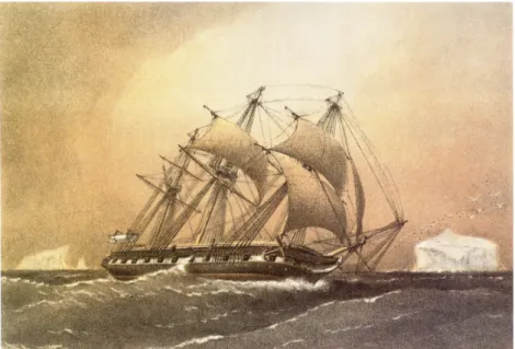
Figure 1.1: The HMS Challenger, a British corvette that took part in the first global marine research expedition: the Challenger Expedition, 1872–1876. Painting by William Frederick Mitchell.

1

http://www.noaa.gov/oceans-coasts

1.1. Underwater challenges

One could say that the underwater exploration started with the Challenger

Expedition (1872, Figure 1.1), by probing the depths from the surface with lead

lines. The Challenger Deep, deepest known point on Earth2_{, has been discovered}

during this expedition. And yet, it was not until the start of the sixties that this spot has been visited by humans, during the dive of the manned submersible Trieste, Figure 1.2. And ever since, the place has been reached by very few expeditions, mainly unmanned descents.

Figure 1.2: Trieste, a Swiss-designed and Italian-built deep-diving research

bathyscaphe. It was able to reach any point of Earth’s abysses such as the

Mariana Trench in 1960. Photo: U.S. Naval Historical Center.

The dive of the Trieste revealed the capacity to build vehicles able to resist

colossal pressures. However, the costs of this endeavor is huge compared to

the range of the explored area: only few square meters around the submersible. And if exploration techniques have evolved considerably over the years, the ratio exploration/cost or exploration/time remains a major impediment in the discovery of our oceans.

Chapter 1. Introduction

1.1.2

Hostile environments

Withstand the high pressures of the column water, corrosive salinity, unpredictable currents, etc., is one thing. However, perceive the environment is another matter. Figure 1.3 provides an example of poor visibility that can be encountered under the surface. Strong opacities in shallow waters, or lack of light in the deepest ones, make it difficult to gather information from cameras. Other conventional means of exploration or communication suffer from strong attenuations of their electromagnetic waves through the water column.

(a) An orange buoy dimly visible at 3m. (b) Unstructured environments.

(c) A lost wireless router. (d) Sea life, leading to outliers.

Figure 1.3: In the shallow waters of La Spezia (Italy) during the SAUC-E competi-tions in the NATO Centre for Maritime Research and Experimentation (CMRE, formerly NURC), 2013–2014. These are images taken by the ENSTA Bretagne’s au-tonomous robot Vici. Design algorithms to automatically analyze these observations remains a challenging task.

1.1. Underwater challenges Underwater acoustics

Underwater acoustics is about the only technology left with sufficient performances to increase the range of visibility. A telling experiment is the Heard Island test performed in 1991 [Munk et al., 1994] and planned in order to test the emission of a man-made acoustic signal throughout the world’s oceans. A special phase modulated signal of 57Hz, emitted from an island located in the southern Indian Ocean, has been received by sixteen sites around the world, some of them based on both coasts of North America. This experiment demonstrated that great distances are reachable by acoustics.

Considering an estimation of the sound celerity profile along the propagation, an acoustic wave is even well suited to perceive distances between the emitter and any obstacle in the environment. In practice, ranges of a few dozen meters are affordable to maintain precision at reasonable energy cost. However, one should note that an acoustic signal rarely propagates in straight line. This impacts

distances’ estimations and may even generate blind zones3_{. Underwater acoustics}

remains nonetheless the most suited approach for wide explorations, but the related solutions are far from being straightforward.

A needle in a haystack

The work on this thesis started on the very same day as the beginning of the underwater search for the lost MH370 aircraft operated by Malaysia Airlines, that presumably disappeared in the southern Indian Ocean in 2014. Despite a tremendous deployment of maritime means, making this multinational search effort the largest and most expensive in aviation history, the aircraft remains unfindable.

From October 2014 to January 2017, an overall survey of 120000km2 of the seafloor

was performed, with unsuccessful results. Given the vast areas involved, this search sadly reveals the difficulty we still have to explore the extent of the seabed.

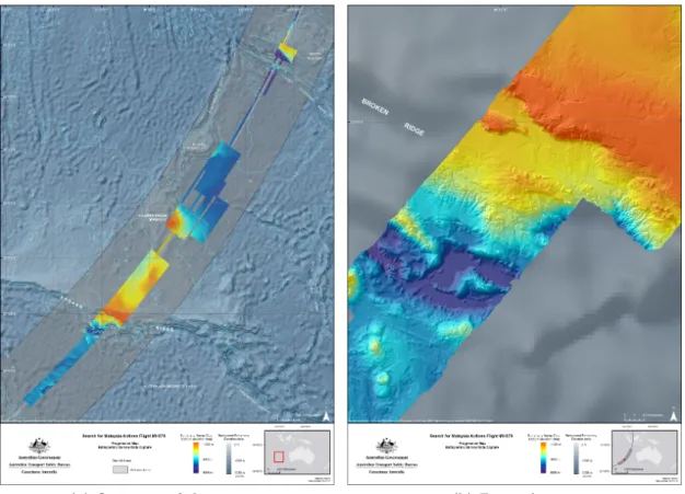
The unfruitful research allowed nonetheless to improve the knowledge we had on this part of the oceans, providing a level of details rarely reached before in the deep environment [Picard et al., 2017]. Figure 1.4 illustrates a comparison between the previous mapping of the seabed, that had an average spatial resolution

3_{In the Atlantic Ocean for instance, due to the physical properties of the environment, two}

vehicles on the same layer of water and separated by 60 meters may not be able to perceive each other.

Chapter 1. Introduction

of about 5km2_{, and the new Digital Elevation Model (DEM) obtained with a}

resolution of less than 0.01km2. During the search, the vessels equipped with

acoustic means such as side-scan sonars or multibeam echosounders were not able to scan the entire extent of the search area. Indeed, the seabed parts with the most complex and challenging topography were only reachable by Autonomous Underwater Vehicles (AUVs), equipped with similar technology and specifically designed for high resolution survey operations in remote deep water locations. These vehicles lend a helping robotic hand in such exploration efforts.

(a) Overview of the survey. (b) Zoomed area.

Figure 1.4: Extract from the bathymetric survey conducted during the search for MH370 aircraft off the west coast of Australia. Gray areas correspond to the bathymetry indirectly estimated using satellite-derived gravity data. In contrast, colored data have been acquired by marine means, highlighting the need to

un-dertake surveys in situ for higher precisions. cCopyright 2014, Commonwealth of

Australia.

1.1. Underwater challenges

1.1.3

Autonomous Underwater Vehicles

Because of difficulties due to complex environments and vast areas still uncovered, the use of autonomous vehicles appears to be a durable solution to face these conditions and push the boundaries of the oceans knowledge. Indeed, even with efficient methods such as underwater acoustics, the footprint of marine sensors is still modest in view of the extent of what has to be explored. Multiply the number of vessels equipped with sensors costs a lot, due to the involvement of crews. On top of that, surface vehicles are not sufficient to provide details of deep waters. Marine robots [Creuze, 2014] are an attractive alternative to increase the exploration means at reasonable costs.

Furthermore, a global supervision of an underwater robot performing an explo-ration task is rarely affordable due to the opacities of the environment mentioned before. The low-rate of underwater communications and the latency during the propagation of messages require the robot a full degree of autonomy. For these reasons, new marine robots are designed to make unsupervised decisions in order to achieve a given task. They can be involved in several marine applications such as hydrography, oceanography, climate change monitoring, military operations in mine hunting [Toumelin and Lemaire, 2001], wrecks search [L’Hour and Creuze, 2016], to name but a few.

As they sail underwater without receiving orders from the surface, they have to sense their environment and act accordingly. AUVs are then equipped with sensors such as sonars or cameras. In addition, they estimate their own position by themselves [Leonard et al., 1998], which is a complicated task as always in the underwater world. The localization problem will be presented in Section 1.2 and is the main motivation of this thesis. The contributions of this work will

be presented through actual experiments involving two AUVs4_{, Redermor and}

Daurade, introduced hereinafter.

4_{The main characters of this document will be drawn by the following as reference to the}

MOOS-IvP middleware [Benjamin et al., 2010] from which this symbol comes from. MOOS-IvP is a set of open source modules for providing autonomy on robotic platforms, in particular autonomous marine vehicles. This framework has been used during this work as basis of actual experiments.

Chapter 1. Introduction The Redermor AUV

The Redermor5 _{AUV, pictured in Figure 1.5, was an experimental robot designed}

during the Franco-British collaborative project Remote Mine Hunting System. Built during the nineties at DGA Techniques Navales Brest (formerly GESMA), it served as platform for several studies [Quidu et al., 2007]. The main characteristics of the vehicle are summarized in Table 1.1, [Toumelin and Lemaire, 2001].

Figure 1.5: The Redermor AUV before a sea trial. The thrusters’ layout allows it to circumnavigate a point such as a mine to identify, its front looking sonar providing different viewing angles of the target. Photo: DGA-TN Brest.

Table 1.1: Redermor ’s main characteristics.

weight : 3400kg

length : 6.40m

speed : up to 10 knots (5.14m/s)

max depth : 200m

During a mission, the position of the robot is provided by an Inertial Navigation System (INS) coupled with a Doppler Velocity Log (DVL) sensing robot’s speed. The positioning error is estimated at some meters per hour. It is difficult to provide the reader with accurate figures about this error as it is related to the pattern followed by the vehicle, its altitude or its speed6_.

5_{Redermor means rider of the seas in the Breton language.}

6_{The DVL accuracy depends among other things on its distance from the seabed and the}

sensed velocity. For a 1200kHz Teledyne DVL, the errors are given as: ±0.3cm/s at 1m/s, ±0.4cm/s at 3m/s, ±0.5cm/s at 5m/s.

1.1. Underwater challenges The Daurade AUV

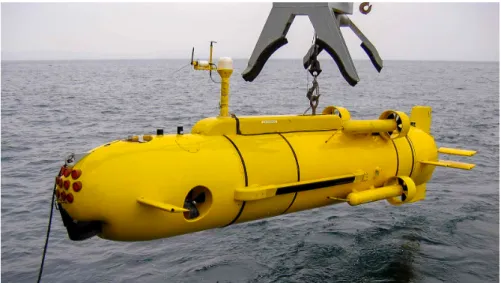
Redermor is today retired and left its place to the new Daurade AUV, see Figure 1.6.

This vehicle has been built by the ECA group and performed many experiments since 2005 on the shores of France. It is still used today by DGA-TN Brest, in

collaboration with the Service Hydrographique et Oc´eanographique de la Marine

(SHOM) for survey purposes or mine hunting applications. Its main characteristics are given in Table 1.2.

Figure 1.6: Daurade AUV managed by the crew of the Aventuri`ere II, during an

experiment in the Rade de Brest, October 2015. Photo: S. Rohou. Table 1.2: Daurade’s main characteristics.

weight : 1010kg

length : 5m

speed : up to 8 knots (4.11m/s)

max depth : 300m

autonomy : 10h at 4 knots, 2h at 8 knots

sonar coverage range : 150m

It is equipped with an INS Phins from iXblue, connected to a DVL7 _{as for the}

Redermor. Its positioning accuracy is 3m/h at 2 knots, or 0.1% of the traveled

distance, based upon a hybridization INS/DVL. On the other hand, 20 meters of positioning error are obtained after 5 minutes of navigation in pure inertial mode.

Chapter 1. Introduction

Redermor and Daurade are heavy vehicles with high costs of handling and

maintenance. Furthermore, the embedded navigation systems cannot be easily changed, which is a limitation when it comes to try new algorithms for autonomous navigation. This motivated the design of smaller and cheaper units.

The Toutatis AUVs project

A new class of autonomous underwater vehicles has been designed during this PhD thesis. The class term refers to a group of several units of the same type.

The Toutatis8 _{project, as Team Of Underwater roboTs for Autonomous Tasks of}

Inspection and Survey, was aimed at applying the tools presented in this document in realistic scenarios. The project has been paused and will be resumed later.

Figures 1.7 picture some modeling views of the vehicles. The units are modular in order to fit with the mission requirements. The aluminium cage protects the tube, the sensors and the thrusters. It is also convenient to arrange devices everywhere on the frame without difficulty. In addition, the cage is useful to carry, transport and store the vehicles; then it will be possible to stow all AUVs on top of each other in a reduced place. Finally, landing on the seabed will not present any risk. Being powered by six thrusters, the AUVs will be omni-directional which is of interest to orient sensors according to the needs. The vehicles should be equipped with cameras, sonars, echosounders, an acoustic modem, a low-cost Inertial Measurement Unit (IMU), a DVL and a pressure sensor.

If it appears clear that AUVs have the potential to revolutionize the means of exploring our oceans, several challenges still remain before considering their active use, the primary of which is the localization problem.

8_{Toutatis is a Celtic god in ancient Gaul and Britain culture. It was seen as the tribe’s leader:}

this name illustrates the future behaviour of these robots: they will act as members of a team, based on communication and collaboration.

1.2. The localization problem

(a) One unit.

(b) A stack of modular vehicles.

Figure 1.7: An overview of the Toutatis AUVs project.

1.2

The localization problem

A robot localization is the process of estimating the vehicle’s position in a given reference frame. This is a key point of mobile robotics as it conditions the success of other processes such as sensing, actuation, manipulation or mapping. In the latter case, a poor positioning estimation will directly lead to datasets acquisitions with meaningless spatial distribution. On top of that, a good localization is mandatory to ensure the safety of the vehicle: for instance when moving in the vicinity of some offshore construction or during the recovery procedure.

In the case of autonomous vehicles, the localization process has to be embedded. Indeed, as soon as a robot dives under the surface, it does not receive electromagnetic

Chapter 1. Introduction

waves anymore. Global Navigation Satellite Systems (GNSSs)9_{, well used in}

terrestrial and aerial applications, cannot be considered in the underwater case. This raises an important amount of work in the community of underwater robotics, in order to investigate new localization techniques. It has led to the design of dedicated sensors and algorithms.

This thesis is a contribution to the localization problem. The current section formalizes the problem and briefly presents already existing positioning approaches in order to place our work with respect to the state of the art and see its main added values. Our motivation being the exploration of wide and unknown underwater areas, we will only consider the generic case of long range navigations without any

prior knowledge10 _{on the environment.}

1.2.1

State equations

The localization algorithms make use of data collected by a set of sensors that we can divide into two categories: proprioceptive measurements and exteroceptive ones. The first one gathers information related to the robot’s state, such as its acceleration, heading, speed, while the second is related to the environment: temperature, distance from a beacon, camera images, etc.

Mathematics provide a way to convert the world into equations. For the localization problem, the following state equations are generally used:

(

˙x(t) = f (x(t), u(t)) ,

z(t) = g (x(t)) .

(1.1a) (1.1b)

Here, x ∈ Rn _{depicts the state of the robot: position, heading, speed, etc.}

We then speak about state estimation as the localization problem amounts to estimating x based on these equations and both proprioceptive and exteroceptive measurements.

9_{At the time of writing, GPS, GLONASS and Galileo are available terrestrial positioning}

systems respectively handled by the United States, Russia and the European Union.

10_{Otherwise, when a given initial map of the environment is available, a process of data}

matching between robot data and the map leads to map-based navigation approaches [Tuohy

et al., 1996, Tyr´en, 1982].

1.2. The localization problem

Equation (1.1a) is differential and depicts the state evolution. f : Rn_×Rm _{→ R}n

is called evolution function. The input vector u ∈ Rm represents the control applied

on x. Measurements are depicted by a vector z ∈ Rp _{related to x through the}

observation function g : Rn_{→ R}p_{, Equation (1.1b). We emphasize that in practice,}

both functions f and g may be uncertain or non-linear. These constraints will be carefully taken into account in this document.

For instance, an underwater robot may be described as x = (x1, x2, x3, ψ, ϑ)|

where x1, x2, x3 are respectively the east, north and vertical positions of the robot,

ψ its heading and ϑ its speed. An onboard pressure sensor will easily provide

pro-prioceptive data about the vertical position of the robot11. However, the estimation

of the horizontal location (x1, x2) is a lot more challenging. We summarize in the

next sections several useful localization methods [Leonard et al., 1998]. Note that

in this document, the horizontal position will sometimes be denoted p = (x1, x2)|

to simplify the reading.

1.2.2

Dead-reckoning drawbacks

Proprioceptive approach

The simplest way to localize one-self is dead-reckoning. From successive proprio-ceptive measurements, a system will estimate its own evolution, step by step. A blind walker would proceed in the same manner by counting its footsteps and then roughly estimating its move. This is the most common localization approach in mobile robotics, as it only requires inner sensors and runs in most environments.

An embedded IMU will provide information on linear accelerations and rotation speeds of the system. Coupled with a magnetometer, the system will also be able to assess its Euler angles: the bank φ, the elevation θ and the heading ψ. The terms

roll φ, pitch θ, yaw ψ are usually employed to depict these orientations. Then, a

dedicated unit called Inertial Navigation System (INS) will provide an estimate of the robot’s state based on these measurements and some algorithms such as a Kalman filter [Kalman, 1960].

External references are not involved in this process. However, in the field of underwater robotics, it is important to mention DVLs that provide information

11_{The estimated depth depends on pressure and water salinity. In the oceans, each 10 meters}

Chapter 1. Introduction

about the vehicle speed. From the emission of acoustic beams, the device will measure velocities within the water column using the Doppler effect. When the beams reach the bottom, measured velocities can be used to compute displacements relative to the seabed. Today, DVLs are well hybridized with marine INSs, which greatly improve performances regarding pure inertial navigations.

Drifting effects

From a known initial position p0, an INS will filter the measurements and estimate

the successive poses of the robot. This is achieved by integrating the motion data in time, sometimes twice in the case of acceleration measurements, which mathematically leads to quadratic errors. For instance, a position estimated by

means of biased acceleration measurements ab(t) = a∗(t) + b is expressed by

pb(t) =

Z Z t

t0

ab(τ )dτ + p0. (1.2)

The bias b is cumulated over time in such a way that the position error is:

e(t) ≈ bt

2

2. (1.3)

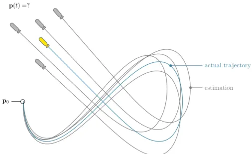
This effect is pictured in Figure 1.8. Unfortunately the drift cannot be bounded and is even substantial when using second order measurements such as accelerations.

The errors can have various causes: noise from sensors, wrong calibrations of the units, a misalignment between the magnetometer and the IMU, etc. In the case of underwater robotics, one must also consider the impact of ocean currents on the vehicle which adds another velocity component poorly sensed by these sensors. Furthermore, without mentioning power consumptions, the cost of an accurate INS may be too excessive for small AUVs. An essential link between an INS and conventional exteroceptive sensors such as sonars has to be contemplated [Dillon, 2016].

Therefore, dead-reckoning methods are not suited for underwater long range navigations. The AUV will have to surface on a regular basis in order to fix its positioning estimation thanks to GNSS signals. This entails risks related to discretion, safety, or even collision with surface vehicles. Furthermore, when AUVs have to operate in very deep waters – as for the MH370 aircraft search – the process of surfacing takes time and energy. Finally, other applications such as exploring ice-covered oceans or karst environments [Lasbouygues et al., 2014] will necessarily require other approaches to perform a long-term localization.

1.2. The localization problem

p(t) =?

p0

actual trajectory

estimation

Figure 1.8: Illustration of drifting state estimations with a dead-reckoning method.

From a known initial position p0, a dead-reckoning method will integrate speed

and inertial measurements which lead to cumulative errors with time. Successive

actual positions are plotted in blue • and four arbitrary estimations are drawn in

gray •.

1.2.3

Underwater acoustic positioning systems

This introduction is not aimed at providing a comprehensive list of dead-reckoning alternatives, but the two following acoustic techniques are widespread enough to be referenced. They will be mentioned afterwards in this document, as part of simulated examples or as a basis of actual datasets.

Basics

Acoustic positioning systems stand on the measurement of signals’ time of flight. Distances between an emitter and a receiver (or an obstacle reflecting the wave) can then be computed assuming a good estimation of the sound velocity profile

through the water column12. The Heard Island experiment demonstrated that

great distances can be reached by acoustics, and even assessed if the sound celerity

12_{The sound celerity profile mainly depends on pressure, salinity and temperature: parameters}

not always well known and that have to be measured in situ. In salt water, the sound travels at about 1500m/s.

Chapter 1. Introduction

profile is sufficiently known along the propagation. However, estimations get complicated in the vicinity of interfaces of two different media, namely water/seabed or water/surface, due to the reflection of waves and multipath interferences. Robust filters have to be used in order to overcome these outliers [Vaganay et al., 1996].

Positioning systems involve acoustic beacons in different configurations, two of which are presented hereinafter. The reader interested in this topic can refer to the literature for additional information [Jensen et al., 2011, Milne, 1983].

Long baseline acoustic positioning systems

A Long BaseLine (LBL) system is made of an array of acoustic transponders deployed on the seabed and precisely geolocalized. The vehicle is also equipped with a transponder in order to trigger the emission of signals from the beacons and receive the feedback. Figure 1.9 illustrates a typical LBL installation.

buoy transponder receiver x1 x2 x3

Figure 1.9: A LBL navigation system made of four hydrophones. The vehicle receives range-only signals and then estimates its position.

A received signal is range-only as it consists in a wave emission that propagates spherically from the emitter. The bearing information (direction-of-arrival data) is not assessed with a single beacon. The position of the vehicle is then estimated at the intersection of the spheres centered on the beacons, each of which with a radius measured from the sound time of flight. The transponder installation can be up to few kilometers wide while providing a positioning accuracy of a few meters. 16

1.2. The localization problem

Of course the deployment of such installation may be expensive, not to mention the duration of the calibration phase that can involve a complete crew. Furthermore, the installation is not suited for wide explorations of several tens or hundreds of kilometers.

Ultra-short baselines

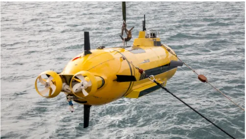
A more mobile approach is the Ultra-Short BaseLine (USBL): a concentrated array of transceivers mounted on the very same device [Pennec, 2010], see for instance the system pictured in Figure 1.10a that has been used during some of the experiments presented in this document.

The device includes a set of acoustic transceivers providing both range and bearing measurements between the USBL and the receiver unit embedded in the vehicle, Figure 1.10b. In this approach, the calibration is made once by the manufacturer, allowing a straightforward use of the device. Furthermore, it can

be settled under a boat localized with an accurate GNSS13_{. The combination of}

these two positioning systems enables the estimation of vehicle’s absolute positions with an accuracy of one meter or below. However, due to the proximity of the transceivers, the angular accuracy may not be sufficiently good to localize a distant vehicle. In addition, the transceivers will usually be located near the surface, suffering from several outliers as pictured in Figure 1.11.

In practice, these devices are well suited for local underwater operations such as docking procedures or when a boat has to monitor an AUV. They cannot be considered as a standalone solution for pure autonomous navigation.

Towards dynamical positioning systems

Recent years have witnessed a new approach for underwater localization involving groups of vehicles and collaborative positioning. Range-only beacons or USBL can be mounted on AUVs in order to follow the exploration progress.

Autonomous vehicles can make use of acoustics to communicate low-rate data and exchange information such as state estimations. Then, new algorithms [Bahr

13_{Some devices such as the GAPS, Figure 1.10a, also include a fiber-optic INS to take into}

Chapter 1. Introduction

(a) USBL mounted on the mission boat. This device is made of four transceivers.

(b) The receiver unit is embedded on top of the AUV among other sensors.

Figure 1.10: A USBL transceiver GAPS from iXblue used during sea experiments with the Daurade AUV. The device is mounted under the boat and provides an estimation of the actual AUV trajectory. Photos: S. Rohou.

1.2. The localization problem -600 -500 -400 -300 -200 -100 0 -100 0 100 200 300 400 500 600 x1 x2

Figure 1.11: An overview of 2D positioning results obtained with a USBL system during an experiment involving the Daurade AUV. Non-filtered acoustic data are

pictured by dots • while the filtered trajectory, obtained with a Kalman filter

and proprioceptive measurements, is plotted with a continuous line •. Numerous

outliers and low ping frequency are the main drawbacks of such system. Note that only a part of the received signals are pictured on this figure, other points are serious outliers located out of the survey area.

Chapter 1. Introduction

et al., 2009, Paull et al., 2014, Seddik, 2015] are employed to perform a decentralized localization of the group items. In this context, AUVs may even play specific roles in order to diversify the data obtained by the group. Namely, some items can stay at the surface to benefit from GNSS signals and assist the deeper vehicles that localize themselves and explore the seabed. In the same approach, a reconfigurable LBL has also been studied in [Matsuda et al., 2012, Matsuda et al., 2015], introducing the concept of alternating landmark navigation: a technique for which USBLs lay on the seabed as fixed points or explore while being localized by the motionless vehicles. This can be seen as a step by step approach where each step is performed by a vehicle laid on the seabed.

While these works achieve promising results, they also raise other difficulties such as the saturation of the acoustic channel, as messages are broadcasted in the same environment.

1.2.4

SLAM: a standalone solution

Another approach for robot localization has received large attention since the early stages in this field [Smith et al., 1990]. The Simultaneous Localization And Mapping

(SLAM)14_{, is an approach that ties together the problem of state estimation and}

the one of mapping an unknown environment.

A chicken and egg problem

We have seen that a dead-reckoning localization necessary leads to uncertain positioning estimations with time. A robot exploring its surroundings will associate these uncertainties to the observed features, assigning their location with some error. However, a scene of the environment may be seen several times during the exploration, which leads to an inter-temporal measurement which could benefit both localization and mapping procedures. Indeed, a robot that recognizes a part of the environment will deduce to be close to a previous position. This is highlighted by the example presented in Figure 1.12.

Hence, these methods consider that positioning and mapping errors are closely related: a concurrent resolution may apply [Leonard and Durrant-Whyte, 1991].

14_{In the literature, SLAM is sometimes referenced as CML: Concurrent Mapping and}

Localiza-tion.

1.2. The localization problem

seamark

Localization of the seamark by the robot

Localization of the robot based on the previous estimation of the seamark p(t1) p(t2)

p0

Figure 1.12: A simple SLAM illustration presenting robot’s positions at two different

times t1 and t2. In pure dead-reckoning, the left part of the image would depict

a precise estimation of the robot’s trajectory while the positioning uncertainties would be strong on the right one. Considering a SLAM approach, a robot coming back to a previous place and perceiving again an object, such as a seamark, will be able to refine its state estimation.

A significant amount of work has been completed around this topic, still subject to further research [Newman and Leonard, 2003, Lemaire et al., 2007].

Loop closure

The key point of SLAM methods is to detect that a place has been previously visited. This problem is known in the literature as loop closure.

It may be difficult for a robot to detect a closure, due to poor estimations on both its position and map-matchings. Worse still, two different objects of same shape may be considered as unique by algorithms standing on too uncertain positioning estimations. Figure 1.13 highlights the case of two identical objects and uncertain trajectory estimates.

Chapter 1. Introduction

seamark A seamark B

actual trajectory

p0

Figure 1.13: A robot flying over two different but same-looking seamarks. The

actual trajectory is plotted in blue • while several dead-reckoning estimations

are drawn in gray •. All the trajectories are consistent with the observations. A

well-known map would not prevent from wrong detections.

This problem is not fully resolved yet. One of the contributions of this thesis is to provide a test to prove that a robot performed a looped trajectory, considering uncertainties from a set of proprioceptive measurements. This work will be presented in Chapter 6 and illustrated in the underwater case through actual experiments involving the previously introduced AUVs. The tool is well suited to prevent from false loop detections in similar environments. It has also other uses such as the reduction of the computational burden of SLAM algorithms.

Computational burden

The complexity of SLAM algorithms quickly increases with the exploration of wide environments, as it implies lots of loop closures to identify among a dense set of data. To this day, the execution of SLAM programs in 3D environments is often not affordable for classical embedded systems powering the robots. A part of the community hence focuses on light-weight solutions, sometimes at the expense of the loss of data associations.

Algorithms involving proprioceptive measurements only are now able to detect 22

1.2. The localization problem

loops without going into a costly analysis of observation datasets [Aubry et al., 2013]. This approach significantly reduces the complexity of SLAM algorithms.

Homogeneous environments

Another challenging issue is the identification of points of interest. Aside from the problem of confusable similar scenes, it is relatively straightforward to recognize artificial objects in terrestrial environments, exploiting high definition cameras and clear visibility of the scenes. A set of ready-to-use image processing libraries already provides efficient results for such applications.

However, points of interest are less identifiable in natural environments. It then requires raw-data approaches that do not stand on the identification of objects. Dealing with underwater environments, globally homogeneous in shape and observable with poor visibility, the only SLAM methods left to the roboticist are raw-data approaches. This thesis provides an original method considering these constraints.

Chapter 1. Introduction

1.3

PhD thesis context

“The necessary knowledge is that of what to observe.”

Complete Tales & Poems, Edgar Allan Poe

What characterizes the underwater case is the paucity of relevant information. This thesis focuses on a new localization approach in such poor environments. The presented method can be characterized as a raw-data SLAM approach, but we propose a temporal resolution – which differs from usual methods – by considering time as a standard variable to be estimated. This concept raises new opportunities for state estimation, under-exploited so far.

However, such temporal resolution is not straightforward and requires a set of theoretical tools in order to achieve the main purpose of localization. This thesis is thus not only a contribution in the field of mobile robotics; it also provides new perspectives in the areas of constraint programming and set-membership approaches.

This section briefly presents the proposed localization method and highlights the intermediate steps investigated during this work, providing the reader an overview of the document structure.

1.3.1

New localization approach in very poor environments

Assumptions

By very poor, we mean environments that do not present land/sea marks or any visible object that could be used as reference. A wide seabed area without recognizable objects such as anchors or wrecks corresponds to such poor environment. By going further, we will even assume that the observation function g is unknown due to too much uncertainties about the environment. Furthermore, we will only consider a static environment which does not evolve during the exploration mission in a non-deterministic manner. Any measurably change of it must be formally known, for instance based on physical models.

1.3. PhD thesis context Inter-temporal approach

Standing on the static environment assumption, a robot coming back to a previous

position p = x1,2 must sense the same observation z as the first time. Formally,

p(t₁) = p(t2) =⇒ z(t1) = z(t2). (1.4)

We propose the following generic formalism:              ˙x(t) = f (x(t), u(t)) , (((( (((( z(t) = g (x(t)), h (x(t₁)) = h (x(t2)) | {z }

same state configurations

=⇒ z(t1) = z(t2) | {z } same observations , (1.5a) (1.5b) (1.5c)

introducing the configuration function h : Rn → Rn0

that depicts a singular configuration of a state. When same configurations are encountered twice at times

t1 and t2, then x(t1) and x(t2) present a singular relation leading to identical

measurements. In this document, we will only focus on the positioning components

p = (x1, x2)| of the state vector, but Equation (1.5c) allows wider applications15.

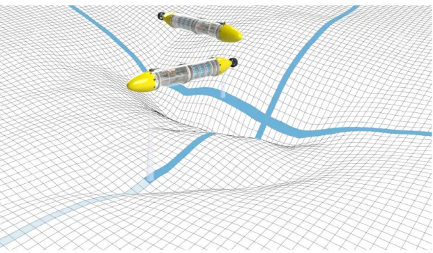
We emphasize that the observation function g is not involved in this formalism. Our illustrations will stand on scalar bathymetric measurements acquired from a single beam echosounder measuring the altitude of the AUV over the seafloor. Figure 1.14 provides a synthesis image of an underwater robot crossing back a previous position. Here, the robot is regulated at constant depth and senses its altitude with a sonar. We will see that other kind of observations can be considered, such as the passive electric sense.

Equation (1.5c) provides a new relation between robot states and observations, as the function g did. The difference is, however, that it links information that can be temporally very distant, even if an analytical expression between x and z is not at hand. According to the resolution method employed to solve the problem, the

time references t1 and t2 could also present uncertainties.

To keep things simple, errors are not represented in Equations (1.5). It is a simple formalism and each resolution method – such as a Bayesian approach or a set-membership estimation – will model the uncertainties in its own way.

15_{For instance, the method should also apply in environments presenting symmetry properties.}

This has been the object of a study Robot localization in an unknown but symmetric environment during this thesis, not detailed in this document.

Chapter 1. Introduction

Figure 1.14: A Toutatis AUV exploring its surroundings with a single beam echosounder. This view presents two instants of the mission, before and after performing a loop. The localization approach defended in this document is based on the constraint raised during the trajectory crossing, where observations should be identical despite their temporal distancing.

1.3.2

Estimation methods

The localization problem modeled by the System (1.5) involves differential equations and functions that can be non-linear. Furthermore, uncertainties have to be propagated over the evolution of the system. As inter-temporal measurements will be the core of the issue, the effects of these propagations over the time intervals must be assessable.

Exact resolution methods cannot apply for this problem as it does not present analytical solutions. Estimation approaches have to be considered. This section presents our motivation for set-membership methods.

1.3. PhD thesis context Probabilistic approaches

These usual methods compute a unique estimated solution with uncertainties qualified by means of covariance matrices [Papoulis and Pillai, 2002]. When dealing with linear equations and uncertainties that are Gaussian-distributed, it has been shown that the well-known Kalman filter [Kalman, 1960] is optimal. Extensions to the non-linear case have been studied afterwards, performing linearizations when necessary. However, this might be a source of estimation errors and it becomes difficult to qualify such uncertainty.

On the other hand, stochastic approaches have received a large attention from the community of automatic and control, providing significant results in the non-linear case [Thrun et al., 2005]. These methods randomly sweep across feasible inputs or parameters and generate a set of probable trajectories: samples. To increase the chances to have one estimation among the samples that is close to the actual solution, a lot of computations have to be attempted. Their probability is evaluated and further samples are then generated in the probable areas based on these likelihoods, allowing a convergence of the algorithm towards a relevant estimation.

However, these random-based computations may badly behave in case of strong non-linearities or few available observations. The risk is to assign a high likelihood to a wrong solution and let the algorithm converge to it. In our localization context, it is essential to address the problem with an estimation method robust to a lack of data and non-redundant information. Probabilistic methods do not seem suited for this purpose.

Set-membership methods

We will pay a specific attention to set-membership approaches that have proved their worth to deal with non-linearities and substantial uncertainties.

“I think it is much more interesting to live not knowing than

to have answers which might be wrong. I have approximate answers and possible beliefs and different degrees of certainty about different things, but I am not absolutely sure of anything and there are many things I do not know anything about. ”

Chapter 1. Introduction

The approach effectively does differ from probabilistic methods in regards of the nature of the estimated solution. Probabilistic methods compute a punctual potential solution – for instance a vector – while in set-membership ones, it is the set of all feasible solutions that is evaluated, and thus an infinity of potential solutions. Another main distinction lies in the way things are computed: with set-membership methods, estimations are not randomly performed. Computations are deterministic: given a set of parameters or inputs, algorithms will always output the same result.

These methods stand on reliable computations over bounds defining ranges of possibilities. Operations are guaranteed not to lose any solution. The main counterpart is that any unlikely solution will be kept in the resulting set if it is consistent with the system’s equations. As a result, algorithms provide pessimistic outcomes and sometimes even meaningless results depending on the situation: “I

am not absolutely sure of anything”.

The maximum distance between the unknown actual solution and any point in the output set is computable and defines the quality of the approximation: it is the worst case error if any point in the set is taken as solution. Therefore, in contrast to the above-mentioned approach, these methods are well suited to reliably propagate uncertainties over the operations.

Conclusion

The problem we are dealing with presents only few observations, especially non-redundant. Capitalize upon them is the key and an accurate resolution method is necessary to never diverge from this information. This is the reason why a set-membership approach is considered in this document. Furthermore, in our un-derwater applications, uncertainties are strong and non-linearities omnipresent, due to range-only observations: these are situations easily managed by this approach. In addition, using set-membership methods will provide guaranteed outcomes, which can be of main interest for the safety of robotic systems [Goubault et al., 2014, Monnet et al., 2016].

Last, but not least, this SLAM problem will be solved in a temporal way, by comparing observations that are temporally distant and considering time references as complete variables. It seems that only a strict and reliable approach can suit. However, set-membership methods do not provide the necessary theoretical tools 28

1.3. PhD thesis context

yet. One of the purposes of this thesis is to extend the methods in order to deal with temporal relations, and apply the proposed tools on our localization problem.

To achieve this resolution, a constraint based approach will be applied. The work motivated by our robotic problem will lead to contributions in the communities of constraint programming and robotics. The theoretical contributions related to the constraints field are briefly motivated in the following section.

1.3.3

Constraint programming approach

over dynamical systems

We have seen that the aim of set-membership approaches is to define a reliable set of feasible solutions. This strategy goes well with constraint propagation techniques: another area widely explored since the 1980’s by a part of the artificial intelligence community [Cleary, 1987, Sam-Haroud and Faltings, 1996]. In particular, we will concentrate on continuous constraints and propose tools to implement new ones in a differential context.

Constraint programming

The constraint programming aims at solving a complex problem by defining it in the form of elementary facts and rules among variables: so-called constraints. A constraint is understood as the expression of any relation that binds variables, which are known to belong to some domains. In our context, constraints may be equalities between physical values as well as non-linear equations, inequalities, or quantified parameters. For instance, the programmer addressing the problem of Equations (1.5), page 25, will list a set of mathematical constraints and will then build a solver. Uncertainties and spaces of solutions are specified either by other constraints or by restricting the domains of the variables. Hence, this approach is in perfect accordance with set-membership methods, benefiting from their reliable operations to apply constraints over sets of values.

In this approach, instead of thinking about how he can solve a problem, the developer will focus on what is the problem, thus leaving the computer to the question of the how. Indeed, each elementary constraint will then be implemented as a black box that does not require any configuration. Constraints can also be easily combined in order to increase in complexity, while preserving simplicity.