HAL Id: lirmm-02067506
https://hal-lirmm.ccsd.cnrs.fr/lirmm-02067506
Submitted on 14 Mar 2019
HAL is a multi-disciplinary open access
archive for the deposit and dissemination of
sci-entific research documents, whether they are
pub-lished or not. The documents may come from
teaching and research institutions in France or
abroad, or from public or private research centers.
L’archive ouverte pluridisciplinaire HAL, est
destinée au dépôt et à la diffusion de documents
scientifiques de niveau recherche, publiés ou non,
émanant des établissements d’enseignement et de
recherche français ou étrangers, des laboratoires
publics ou privés.
Measurement and Generation of Diversity and
Meaningfulness in Model Driven Engineering
Adel Ferdjoukh, Florian Galinier, Eric Bourreau, Annie Chateau, Clémentine
Nebut
To cite this version:
Adel Ferdjoukh, Florian Galinier, Eric Bourreau, Annie Chateau, Clémentine Nebut. Measurement
and Generation of Diversity and Meaningfulness in Model Driven Engineering. International Journal
On Advances in Software, IARIA, 2018, 11 (1/2), pp.131-146. �lirmm-02067506�
Measurement and Generation of Diversity and
Meaningfulness in Model Driven Engineering
Adel Ferdjoukh
LS2N & University of Nantes, France adel.ferdjoukh@univ-nantes.fr
Florian Galinier
IRIT, University Paul Sabatier, Toulouse. France florian.galinier@irit.fr
Eric Bourreau, Annie Chateau
and Cl´ementine Nebut
Lirmm, CNRS & University of Montpellier, France
lastname@lirmm.fr
Abstract—Owning sets of models is crucial in many fields, so as to validate concepts or to test algorithms that handle models, model transformations. Since such models are not always available, generators can be used to automatically generate sets of models. Unfortunately, the generated models are very close to each others in term of graph structure, and element naming is poorly diverse. Usually, they badly cover the solutions’ space. In this paper, we propose a complete approach to generate meaningful and diverse models. We use probability simulation to tackle the issue of diversity inside one model. Probability distributions are gathered according to domain quality metrics, and using statistical analysis of real data. We propose novel measures to estimate differences between two models and we provide solutions to handle a whole set of models and perform several operations on these models: comparing them, selecting the most diverse and representative ones and graphically observe the diversity. Implementations that are related to difference measurement are gathered in a tool namedCOMODI. We applied these model comparison measures in order to improve diversity in Model Driven Engineering using genetic algorithms.
Index Terms—Model Driven Engineering; Intra-model Diver-sity: Inter-model Diversity; Meaningfulness of Models; Counting Model Differences.
I. INTRODUCTION& MOTIVATIONS
The present paper is an extended version of the paper that the authors published in ICSEA’2017 conference [1].
The increasing use of programs handling models, such as model transformations, more and more increases the need for model benchmarks. Elements of benchmarks are models expected to respect three quality criteria at the same time. First, they must be as representative as possible of their domain-specific modelling language. Then, they have to be diverse in order to chase the potentially rare but annoying cases where programs show a bad behaviour. Finally, they must be meaningful and close to hand-made data in some aspects. The difficulty of finding real test data that fulfil all these requirements, and in sufficient quantity to ensure statistical significances, leads to consider the automated generation of sets of models. Many approaches and tools can be used in this purpose: Ferdjoukh et al. [2], Sen et al. [3], Cabot et al. [4], Gogolla et al. [5].
We distinguish two different concepts of diversity.
Intra-model diversityensures that the elements contained in a single
model are sufficiently diverse. For example, when generating a skeleton of a Java project, we verify that there are many packages in the project. The packages should contain diverse numbers of classes. Classes should contain fields and methods of diverse types, etc. Inter-model diversity forces two models taken as a pair to be as different as possible. With a possible extension to a whole set of models. The combination of these two different kinds of diversity guarantees both the well coverage of the meta-model’s solution space and the meaningfulness of the generated models.
Intra-model diversity is linked to the concept of
mean-ingfulness for models. Thus in the previous example, let us consider that the classes of a Java project are all concentrated in one package. We estimate that this project is not well-formed or meaningful. In practice, this kind of project does not respect Object Oriented Programming quality criteria, because its reusability is poor. In this paper, we propose to use probability distributions related to domain-specific quality metrics to increase the intra-model diversity.
One of the main issues when attempting to produce different models, is to state in what extent, and according to which criteria, the models are actually “different”. The most natural way to formalize this notion, is to define, and use metrics comparing models, and measuring their differences.
Determining model differences is an important task in Model Driven Engineering. It is used for instance in repos-itories for model versioning. Identifying differences between models is also crucial for software evolution and maintain-ability. However, comparing models is a difficult task since it relies on model matching. This latter can be reduced to graph isomorphism that is an NP-intermediate problem (No polynomial algorithm is known for Graph isomorphism problem, but it has not been proven NP-complete. The more general sub-graph isomorphism problem is NP-complete.) [6]. Kolovos et al. [6] draw up an overview of this issue and give some well-known algorithms and tools for model comparison. Most of these approaches compare only two models between them and find their common elements. This is insufficient for
the problem of diversity improving because differences have to be measured and a whole set of models has to be considered. In this work, we propose a distance-based approach to measure model differences and we provide solutions to handle sets of models in order to compare them and to extract the most representative models. A human readable-graphical viewing is also given to estimate the diversity of a set of models.
We consider models, which are conform to meta-models, according to the Ecore/EMF formalization [7]. Model
genera-tion is performed using
G
RIMM[2], [8], [9], [1] and it is basedon Constraint Programming [10]. Basically,
G
RIMM reads ameta-model and translates all elements of the meta-model into a Constraint Satisfaction Problem (CSP). A CSP solver is then used to solve the obtained constraint network, leading to one or more models, which are conform to this meta-model, and meeting a given set of additional parameters describing the characteristic of desired models. Constraint Programming provides a deterministic behavior for the generation, it is then difficult to encode diversity directly in the heart of the tool. Other model generation tools can be coupled with our approach. For example, during our experiment we also used
models that have been generated using PRAMANA tool (Sen
et al. [3]). We investigate in this work the use of genetic algorithms, so as to diversify an obtained set of models (the preliminary elements for the approach can be found in [11]). In summary, our contributions are: (1) an approach for in-creasing intra-model diversity based on probability simulation (2) two case studies to show the efficiency of the previous method (3) novel metrics measuring model differences using distances coming from different fields (data mining, code correction algorithms and graph theory) and adapted to MDE (Model Driven Engineering) (4) solutions to handle a whole set of models in order to compare them, to extract the most representative models inside it and to give a graphical viewing for the concept of diversity in MDE (5) A tool implementing these two previous contributions (6) an application of these distance metrics in improving inter-model diversity in MDE using a genetic algorithm.
The rest of the paper is structured as follows. Section II
relates about previous literature. Section III presents
G
RIMM,our methodology and tool for automated generation of models. Section IV describes how we face the issue of intra-model diversity in MDE. Two case studies show the efficiency of the previous approach (Section V). Section VI details the considered model comparison metrics. Section VII details the solutions for handling a set of models (comparison, selection of representative model and graphical viewing). The tool implementing these contributions is described in Section VIII. An application of our method to the problem of inter-model diversity in MDE is shown in Section IX. Section X concludes the paper.
II. RELATED WORK
This section draws a state of the art of the topics related to the work we presented in our paper. Related work is divided
into three parts. Each part relies on one important contribution of this paper.
A. Meaningful models
We give here a short list of approaches for model generation. Many underlying techniques have been used. Cabot et al. [12] translate a meta-model and its OCL constraints into constraint programming. In [13], Mougenot et al. use random tree generation to generate the tree structure of a model. Wu
et al. [14] translate a meta-model into SMT (Satisfiability
Modulo Theory) in order to automatically generate conform models. In [15], Ehrig et al. transform a meta-model into a graph grammar, which is used to produce instances. The advantages and drawbacks of our original approach relatively to the other generating methods have been discussed in [8].
Nevertheless, only two approaches have treated the problem of meaningfulness of generated models. In [13], authors use a uniform distribution during the generation process and add weights in order to influence the frequency of appearance of different elements. In [14], authors describe two techniques to obtain relevant instances. The first one is the use of partition-based criteria, which must be provided by the users. The second one is the encoding of common graph-based properties. For example, they want to generate acyclic graphs,
i.e.,models.
B. Model comparison
The challenging problem of model comparison was widely studied, many techniques and algorithms were proposed for it. Two literature studies are proposed in [6] and [16]. Among all the techniques, we describe here the techniques that are close to the model distance algorithms we propose, in both comparison and objective.
Falleri et al. [17] propose a meta-model matching approach based on similarity flooding algorithm [18]. The goal of this approach is to detect mappings between very close meta-models to turn compatible meta-models, which are conform to these meta-models. The comparison algorithm detects two close meta-models. A transformation is then generated to make the models of the first meta-model conform to the second one. However, in such kind of work, the similarity between models cannot be detected without using the names of elements: lexical similarities are propagated through the structure to detect matchings. Our approach is more structural.
Voigt and Heinze present in [19] a meta-model matching approach. The objective is very close to the previous approach. However, the authors propose a comparison algorithm that is based on graph edit distance. They claim that it is a way to compare the structure of the models and not only their semantics as most of techniques do.
C. Diversity of models
Cadavid et al. [20] present a technique for searching the boundaries of the modeling space, using a meta-heuristic
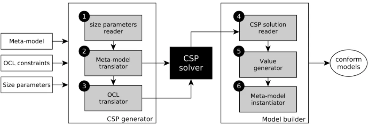
Fig. 1. Steps for model generation usingGRIMMtool.
method, simulated annealing. They try to maximize cov-erage of the domain structure by generated models, while maintaining diversity (dissimilarity of models). In this work, the dissimilarity is based on the over-coverage of modeling space, counting the number of fragments of models, which are covered more than once by the generated models in the set. In our work, the objective is not to search the boundaries of the search space but to select representative and diverse elements in the whole search space.
More recently, Batot et al. [21] proposed a generic frame-work based on a multi-objective genetic algorithm (NSGA-II) to select models sets. The objectives are given in terms of coverage and minimality of the set. The framework can be specialized adding coverage criterion, or modifying the minimality criterion. This work of Batot et al. confirms the ef-ficiency of genetic algorithms for model generation purposes. Our work is in the same vein but focuses on diversity.
Sen et al. [22] propose a technique on meta-model frag-ments to ensure that the space of solutions is well-covered. The diversity is obtained by diversifying the possible cardinalities for references. For example, if a reference has cardinality 1..n, 3 different configurations are considered: 1, 2 and n. To generate a model, the different configurations for all references are mixed.
Hao Wu [14] proposes an approach based on SMT
(Satis-fiability Modulo Theory) to generate diverse sets of models.
It relies on two techniques for coverage oriented meta-model instance generation. The first one realizes the coverage criteria defined for UML class diagrams, while the second generates instances satisfying graph-based criteria.
Previous approaches guarantee the diversity relying only on the generation process. No post-process checking is performed on generated model sets to eliminate possible redundancies or to provide a human-readable graphical view of the set.
III. BACKGROUND:
G
RIMM TOOLG
RIMM(G
eneRatingInstances ofMeta-Models) is a modelgeneration approach and tool. Its goal is the automated genera-tion of instances that conform to ecore meta-models. It is based
on Constraint Programming (CSP) [10]. Schema on Figure 1
shows the steps for model generation using
G
RIMM tool.A. Input
Meta-modelis written using the Ecore formalization. It mainly
contains classes, attributes and references (links between two classes). A class can have one or more subclasses and also one or more super-classes. A reference between two classes can be bi-directional or unidirectional only. Some references are compositions. One class of the meta-model plays the leading role of root class. It has the particularity of being linked to all other classes by composition relations (directly of transitively).
OCL constraints are additional constraints that come with a
meta-model. They help to disambiguate some elements of the meta-model. OCL is a first order logic language. In our work we are considering only invariants and not all the types of OCL constraints. The area of OCL our tool can handle is large but not complete. We can process simple OCL constraints on one or more attributes, many operations on collections and some typing operations. It is also possible using CSP to take into account some complex and nested OCL constraints.
Size Parameters fix the size of desired generated models.
These parameters are chosen by the user. He fixes the number of instances for each class and unbounded references and also can give the domain of values for an attribute.
B. Processing
Size parameters reader This module of our tool reads a
file containing all the size parameters given by a user and verifies their well-formedness. It also does some inference when information is missing (for attributes values and for unbounded references).
Meta-model translator The goal of this step is to create a
Constraint Satisfaction Problem (CSP) to solve the model generation problem. This module uses the previous size pa-rameters and translates each element of the meta-model (class,
attribute, link, inheritance) into its equivalent in CSP. Much more details about the translation process can be found in [2], [8].
OCL translatorThis step is devoted to the translation of OCL
constraints into CSP. The CSP obtained in the previous step is completed to integrate OCL. Many constructions of the OCL language are taken into account. Simple and complex constraints with one or more attributes are handled. Many widespread operations on collections or on types are also considered. In addition, processing of some nested constraints is possible using Constraint Programming. Translation of OCL constraints is detailed in [8].
CSP solver It is a program that solves CSP. Its goal is to
quickly find a solution satisfying all the constraints at the same time, yielding difficulties when trying to generate diverse and different solutions. Indeed, a CSP solver is designed to quickly find a solution without considering its intrinsic quality or a global vision of all the possible solutions. In other words, although a solution is correct for a CSP solver, it is not necessarily a meaningful model.
CSP solution reader Once a solution is found,
G
RIMM readsthis solution and extracts the values for the model’s elements: inheritance, links and attributes.
Value generatorThe values of some elements are missing after
the previous step. Because CSP handles only integer variables. For other data types: enumerations characters, strings and floats, post-processing is needed. This steps is then crucial to get a complete model.
Meta-model instantiatorThis final step gathers all information
of previous step and builds a valid and conform model. The result of this process is the generation of instances for
meta-models.
G
RIMM tool is able to produce two differentoutputs:
• xmi model files, that can be used for testing model
transformations.
• dotis a format for creating graphs. Our tool uses its own
syntax, so models can be graphically visualized in pdf or png.
The following sections describe contributions for improving the meaningfulness and the diversity of generated models.
IV. INTRA-DIVERSITY OF MODELS
One remaining issue is related to the meaningfulness of generated models. Indeed, we have to produce models that are as realistic as possible, regarding to the data they are supposed to simulate. We propose to use intra-model diversity to achieve this goal.
The declarative approach (CSP) is intrinsically determin-istic, since the solver follows a deterministic algorithm to produce a unique solution. The CSP solver can easily pro-duce thousands of solutions, but they are often far from the
reality. In other words, it is impossible using a combinatorial approach, such as CSP, to express the meaningfulness. It is more a probabilistic concept.
Generation process is enriched with various parameters. We exploit the flexibility of CSP and the fact that some elements of the real models follow usual probability distributions. These distributions are simulated and, a priori, injected to the CSP, in order to produce generated models closer to real ones.
For better results, probability distributions are not arbitrary. They are domain-specific. Indeed, we observe, that many quality metrics are encoded in the meta-models. For example, in Java meta-model, we find an unbounded reference (0..∗) between class and method. It determines the number of methods belonging to a given class. This number is fixed by the CSP solver according to user’s choice. In real models, the number of methods per class is diverse, not constant, and there exist related quality metric [23] and code smells [24]. Our idea is to exploit the metrics, that are encoded in the meta-model, to improve the meaningfulness of generated models.
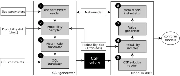
Schema on Figure 3 shows the steps for generation of meaningful models, by exploiting domain specific metrics, and related probability distributions.
A. Input
Probability distributions on linksformally define the diversity,
while linking class instances inside the generated models. For each reference, identified as related to a quality metric, the user defines a probability law (normal, exponential, etc). This law is then used to fix the number of target elements for each class instance. Figure 2 illustrates the diversity, while linking the elements of a model. In the left side, we can see a theoretical model without any diversity. Each circle is always linked to 2 squares. The right side shows a model, in which each circle is linked to a different number of squares.
Fig. 2. Illustrating the diversity while linking elements in a model.
Probability distributions on attributes concern the most
im-portant attributes in a meta-model. For example, in the Java meta-model, the visibility of fields and methods is important. Indeed, object-oriented programming promotes encapsulation. This means that most of fields are private and most of methods are public. The probability laws determine here the value of attribute visibility for each created field and method. A probability is defined for each possible value, and simulation will choose adequate values and assign them to class instances.
Fig. 3. Steps for meaningful model generation usingGRIMMtool.
The parameters for probability distributions are very im-portant for the generation process. Our approach allows the user to choose them arbitrary. Nevertheless, we think that it is preferable to infer them by conducting an empirical study over existing data, or to use domain quality metrics.
B. Probability sampler
Generating samples of well-known probability distributions is a way to add randomness to the deterministic CSP solving process. The idea is to get models that have more diversity in their elements’ degrees and their attributes’ values in order to cover a lot of possible values. For example, when generating UML models, we want to generate a package, which has 5 classes, another one with 7 classes and so on.
Figure 4 shows the basic operation with which we can sample all usual probability distributions whatever they are continuous or discrete. Thus, to generate a sample of a random variable X we need its cumulative function F(X) and a sample of uniform values u. Result values x are obtained by an
inversion of F: u= F(x) ⇒ x = F−1(u).
Previous method is then adapted to each probability distri-bution we want to sample.
Discrete distribution on a finite set For all discrete distri-bution, are given the probabilities of a finite set of values. The cumulative function is then deduced from the accumulation of probabilities and a sample can be easily generated.
Inverse cumulative function method This method is used for continuous distribution if their inverse cumulative function is easily computable. This method is used to simulate the exponential distribution (ε(λ)).
Normal distribution: Box Muller transform Sometimes, inverting a cumulative function is difficult. In these cases, special algorithms are used. For example, a normal distribution
(
N
(µ, σ)) does not have a known inverse function, so previousmethod is useless. However, many other methods exist to
X F(X) 0 1 u x given compute
Fig. 4. Simulation of random values x given a cumulative function F(X) of a random variable X and uniform u
simulate a normally distributed sample. Our implementation uses Box Muller algorithm.
For a more complete overview about probability and simu-lation, please refer to [25].
This section described the method we use to improve the meaningfulness of generated models. We exploit domain-specific quality metrics, and the simulation probability dis-tributions to achieve our goal.
V. CASE STUDIES
This section experimentally shows that using probabil-ity distributions improves the meaningfulness of generated datasets. We consider two case studies, one from Software Engineering area and the other from Bioinformatics.
A. Java code generation
One of the main objectives of our approach is the generation of benchmarks of test programs for different applications, such as compilers or virtual machines. In this experiment, we generate realistic and relevant skeletons of Java programs using real code measurements. We choose Java for facility to find real programs to collect desired measurements. However, our method can be applied to any programming language.
We collected 200 real Java projects coming from two corpus (Github and Qualitas corpus [26]. For more heterogeneity, we
TABLE I. Chosen code metrics with their theoretical probability distribution. ε: Exponential distribution,N: Normal distribution.
Metric Theoretical distrib.
Class/Package ε( 1 8.387) Methods/Type ε( 1 7.06) Attributes/Type N(3.46, 2.09) Constructor/Type N(0.73, 0.26) Sub-Classes/Classe ε( 1 0.22) % Interface/Package ε(8.0011 ) Parameters/Methods N(0.87, 0.25)
chose projects having different sizes (big project for qualitas corpus and smaller ones from github) and different origins (well-known software such as Eclipse, Apache or ArgoUML and also small software written by only one developer). We measured metrics related to their structure, such as the percentage of concrete classes/ abstract classes, the average number of constructors for a class, the visibility of fields and methods, etc [23]. To measure these metrics we used an open source tool called Metrics [27]. After that, we use R software [28] to compute histogram of each metric in order to deduce its theoretical probability distribution. Table I gives the different metrics and their theoretical probability distributions. Figures 5 and 6 show two examples of real corpus histograms.
According to these metrics, we automatically generate Java programs having the same characteristics as the real ones. To achieve this goal, we design a meta-model representing skeletons of Java projects and we adjoin some OCL constraints (about 10 constraints have been added to the Java meta-model we designed). For example:
• All classes inside a package have a different name.
• A class cannot extend itself.
Finally, 300 Java projects are generated using three versions of our approach. Then, we obtain four corpus:
1) Projects generated by
G
RIMM but without OCL.2) Projects generated by
G
RIMM plus OCL.3) Projects generated by
G
RIMMplus OCL and probabilitydistributions (denoted
G
R RIMM in figures).4) Real Java projects.
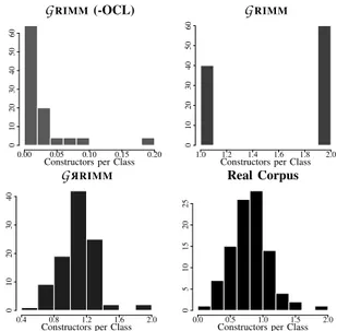
We compare, for these four cases, the distributions of constructors per class and the visibility of attributes in Figures 5 and 6.
We observe that the two first versions without probability distributions give results that are very far from the characteris-tics of real models. On the other hand, introducing simulated probability distributions leads to substantial improvement. We see that the distribution of the number of constructors and the visibility of attributes (Figures 5,6) of generated models are close to real ones. Moreover, these results are always better when adding probabilities for all other measurements presented in Table I.
GRIMM (-OCL)
Constructors per Class
0.00 0.05 0.10 0.15 0.20 0 10 20 30 40 50 60 GRIMM
Constructors per Class
1.0 1.2 1.4 1.6 1.8 2.0 0 10 20 30 40 50 60 G R RIMM
Constructors per Class
0.4 0.8 1.2 1.6 2.0 0 10 20 30 40 Real Corpus
Constructors per Class
0.0 0.5 1.0 1.5 2.0 0 5 10 15 20 25
Fig. 5. Comparing the number of constructors per class in Java projects.
private public protec. package
GRIMM (-OCL) 0 20 40 60 80 100
private public protec. package
GRIMM 0 20 40 60 80 100
private public protec. package
G R RIMM 0 10 20 30 40 50
private public protec. package Real Corpus 0 10 20 30 40 50
Fig. 6. Comparing the visibility of attributes in Java projects.
Despite these encouraging results, some threats to the validity of this experiments can be given. A first one is a construction threat related to the chosen metrics. Indeed, a lot of metrics can be found in the literature. In our experiment we choose only those related to the structure of a project. There is a second internal threat concerning real Java corpus. They may not be sufficiently representative of all the Java projects even if they come from a well-known corpus and a famous repository.
B. Scaffold graphs generation
Scaffold graphs are used in Bioinformatics to assist the reconstruction of genomic sequences. They are introduced late in the process, when some DNA sequences of various lengths, called contigs, have already been produced by the assembly step. Scaffolding consists in ordering and orienting
the contigs, thanks to oriented relationships inferred from the initial sequencing data. A scaffold graph is built as follows: vertices represent extremities of the contigs, and there are two kind of edges. Contig edges link both extremities of a given contig (strong edges in Figure 8), whereas scaffolding edges represent the relationship between the extremities of distinct contigs. Contig edges constitute a perfect matching in the graph, and scaffolding edges are weighted by a confi-dence measure. Those graphs are described and used in the scaffolding process in [29] for instance. The scaffold problem can be viewed as an optimisation problem in those graphs, and consists in exhibiting a linear sub-graph from the original graph. Therefore, it can be considered as well as a model trans-formation, when models conform to the Scaffold graph meta-model given in Figure 7, that we designed. Producing datasets to test the algorithms is a long process, somehow biased by the choices of the methods (DNA sequences generation, assembly, mapping), and there does not exist a benchmark of scaffold graphs of various sizes and densities. Moreover, real graphs are difficult and expensive to obtain. Thus, it is interesting to automatically produce scaffold graphs of arbitrary sizes, with characteristics close to the usual ones. In [29], the authors present some of these characteristics, that are used here to
compare the
G
RIMM instances vs. the ”hand-made” graphs.Fig. 7. A meta-model for the scaffold graphs.
The probability distribution chosen to produce the graph emerges from the observation that the degree distribution in those graphs is not uniform, but follows an exponential dis-tribution. We compare several datasets, distributed in several classes according to their sizes:
1) Graphs generated by
G
RIMM plus OCL.2) Graphs produced by
G
RIMM plus OCL and probabilitydistributions (denoted
G
R RIMM in figures).3) Real graphs of different species, described in [29]. For each real graph, 60 graphs of the same size are auto-matically generated. 30 graphs are naively generated using the
original
G
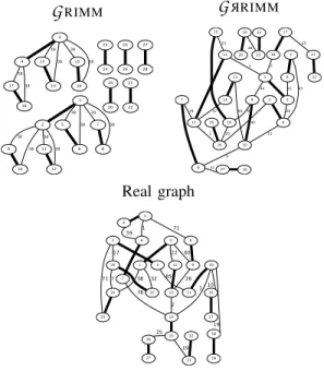
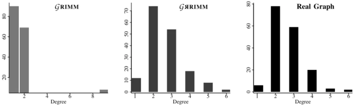
RIMM method [8], [2], and 30 others are generatedafter the simulating of probability distribution. These models are then compared in term of visual appearance (Figure 8), degree distribution (Figure 9) and according to some graph measurements (Table II).
We see in Figure 8 three models (scaffolds graphs) cor-responding to the same species (monarch butterfly). More
1 2 5 38 6 38 7 38 8 38 9 38 10 38 11 38 12 38 3 4 13 38 14 38 15 38 16 38 17 38 18 38 23 24 25 26 27 28 19 20 21 22
G
RIMM 1 2 9 44 6 26 10 16 9 13 3 45 4 41 5 26 42 8 5 7 12 34 27 41 2 28 20 11 5 13 50 14 37 15 23 17 18 21 45 3 22 19 20 23 38 24 25G
R RIMM 0 1 9 60 12 22 21 32 24 38 2 3 20 17 25 71 11 85 4 5 6 59 1 8 71 7 14 78 13 26 10 1 16 10 18 19 2 15 23 19 26 25 17 19 7 22 27 Real graphFig. 8. Three Scaffold graphs corresponding to the same species (monarch butterfly). Strong edges represent contig edges, other edges are scaffolding
edges.
precisely, it refers to mitochondrial DNA of monarch butterfly. The naive method generates a graph that does not look like the real one. This graph is too weakly connected, and the connected parts have a recurring pattern. This is not suitable for a useful scaffold graph. Whereas, introducing probabilities provides graphs having shapes close to reality. Thus, both real graphs and generated graphs (with probability distribution) are strongly connected, and more randomness can be observed in the connections and the weights of edges.
Figure 9 compares the degree distributions for three scaffold graphs of the same species. We see that generating with probabilities gives a distribution very similar to the distribution in the real graph.
Table II compares the three benchmarks of scaffold graphs (naive generation, generation with probabilities and real graphs) according to some graph measurements. We can observe again, that the graphs generated with probabilities are closer to real graphs than the naively generated graphs in all cases. The measurements on the naive graph suffer from a lack of diversity and randomness. Indeed, the minimal and the maximal degree are the same for all generated models. This, of course, does not reflects the reality. Notice also that it was not possible with the naive generation method to generate largest graphs corresponding to largest genomes.
This section presented two different case studies, to show how we exploit domain-specific metrics, for improving mean-ingfulness of generated models. The following sections are devoted to the second aspect of our contributions. It describes the approach we developed to increase inter-model diversity.
2 4 6 8 20 40 60 80 Degree GRIMM 1 2 3 4 5 6 0 10 20 30 40 50 60 70 Degree G R RIMM 1 2 3 4 5 6 0 20 40 60 80 Degree Real Graph
Fig. 9. Comparing the degree distribution between a real scaffold graph and its equivalent generated ones (168 nodes and 223 edges). TABLE II. Comparing graph metrics on real scaffold graphs and average for 60 generated ones for each species.
Graph size Measurements
GRIMM generation G R RIMMgeneration Real graphs Species nodes edges min/maxdegree h-index min/maxdegree h-index min/maxdegree h-index monarch 28 33 1/9 3 1/ 4.6 4.06 1/ 4 4 ebola 34 43 1/9 3 1/ 4.83 4.60 1/ 5 4 rice 168 223 1/9 8 1/ 6.03 5.93 1/ 6 5 sacchr3 592 823 1/9 10 1/ 7 6.76 1/ 7 6 sacchr12 1778 2411 − − 1/ 7.53 7 1/10 7 lactobacillus 3796 5233 − − 1/ 8.06 7.8 1/12 8 pandora 4092 6722 − − 1/ 8.23 7.96 1/ 7 7 anthrax 8110 11013 − − 1/ 8.3 8.03 1/ 7 7 gloeobacter 9034 12402 − − 1/ 8.46 8 1/12 8 pseudomonas 10496 14334 − − 1/ 8.43 8 1/ 9 8 anopheles 84090 113497 − − 1/ 8.96 9 1/ 51 12
VI. MEASURING MODEL DIFFERENCES
Brun and Pierantonio state in [30] that the complex
prob-lem of determining model differences can be separated into three steps: calculation (finding an algorithm to compare two models), representation (result of the computation being represented in manipulable form) and visualization (result of the computation being human-viewable).
Our comparison method aims to provide solutions to com-pare not only two models between them but a whole set of models or sets of models. The rest of this section describes in details the calculation algorithms we choose to measure model differences. Since our method aims to compare sets of models, we took care to find the quickest algorithms. Because chosen comparison algorithms are called hundreds of time to manipulate one set containing dozens of models.
As a proof of concept, we consider here four different distances to express the pairwise dissimilarity between models. As stated in [31], there is intrinsically a difficulty for model metrics to capture the semantics of models. However, formaliz-ing metrics over the graph structure of models is easy, and they propose ten metrics using a multidimensional graph, where the multidimensionality intends to partially take care of semantics on references. They explore the ability of those metrics to characterize different domains using models. In our work, we focus on the ability of distances to seclude models inside a set of models. Thus, we have selected very various distances, essentially of 2 different area: distances on words (from data
mining and natural language processing) and distances on graphs (from semantic web and graph theory). Word distances have the very advantage of a quick computation, whereas graph distances are closer to the graph structure of models. As already said, an interesting feature is the fact that all those distances are, in purpose, not domain-specific, not especially coming from MDE, but adapted to the latter.
A. Words distances for models
We define two distances for models based on distances on words: the hamming distance and the cosine distance. The first one is really close to syntax and count the number of difference between two vectors. The second one is normalized and intends to capture the multidimensional divergence between two vectors representing geometrical positions.
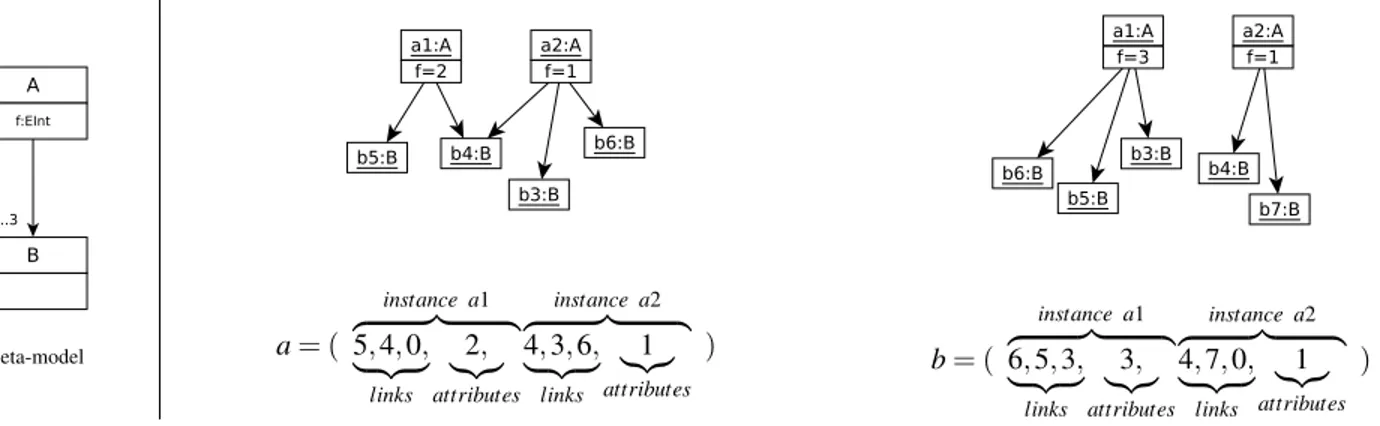
1) From models to words: We define the vectorial
rep-resentation of a model as the vector collecting links and attributes’ values of each class instance, as illustrated on the model of Figure 10. At the left-hand-side of the figure is an example of meta-model. At the right-hand-side of the figure are two models conform to this meta-model, and their vectorial representation. The obtained vector from a model m is composed of successive sections of data on each instance of m, when data is available. Each section of data is organized as follows: first data on links, then data on attributes. When there is no such data for a given instance, it is not represented. In the example of Figure 10, instances of B, which have
Meta-model a= ( instance a1 z }| { 5, 4, 0, | {z } links 2, |{z} attributes instance a2 z }| { 4, 3, 6, | {z } links 1 |{z} attributes ) b= ( instance a1 z }| { 6, 5, 3, | {z } links 3, |{z} attributes instance a2 z }| { 4, 7, 0, | {z } links 1 |{z} attributes )
Fig. 10. Two small models and their vectorial representation.
no references and no attributes, as imposed by the meta-model, are not directly represented in the vectors. However, they appear through the links attached to instances of A. An attribute is represented by its value. A link from an instance i to an instance j is represented by the number of the referenced instance j. Each instance of a given meta-class mc, are represented by sections of identical size. Indeed, all the instances of mc have the same number of attributes. The number of links may vary from an instance to another, but a size corresponding to maximal cardinality is systematically attributed. This cardinality is either found in the meta-model or given in the generation parameters. When the actual number of links is smaller than the maximal number of links, 0 values are inserted.
2) Hamming distance for models: Hamming distance
com-pares two vectors. It was introduced by Richard Hamming in 1952 [32] and was originally used for fault detection and code correction. Hamming distance counts the number of differing coefficients between two vectors.
The models to compare are transformed into vectors, then we compare the coefficients of vectors to find the distance between both models:
a = (5, 4, 0, 2, 4, 3, 6, 1)
b = (6, 5, 3, 3, 4, 7, 0, 1)
d(a,b) = 1+ 1+ 1+ 1+ 0+ 1+ 1+ 0
= 68
Richard Hamming’s original distance formula is not able to detect permutations of links, which leads to artificially higher values than expected. In our version, we sort the vectors such as to check if each link exists in the other vector. In
the previous example, the final distance then equals to 58.
The complexity is linear in the size of models, due to the vectorization step. Notice also that this distance implies that vectors have equal sizes. This is guaranteed by the way we build those vectors.
3) Cosine distance: Cosine similarity is a geometric
mea-sure of similarity between two vectors, ranging from -1 to 1: two similar vectors have a similarity that equals 1 and two diametrically opposite vectors have a cosine similarity of −1. Cosine similarity of two vectors a and b is given by the following formula: CS(a, b) = a.b ||a||.||b||= n ∑ i=1 ai.bi rn ∑ i=1 a2i. r n ∑ i=1 b2i
After a vectorization of models, cosine similarity is then used to compute a normalized cosine distance over two vectors [33]:
CD(a, b) =
1 −CS(a, b)
2
Again, the time complexity of the computation is linear in the size of models.
4) Levenshtein distance for models: Levenshtein distance
[34] (named after Vladimir Levenshtein) is a string metric used to compare two sequences of characters. To summarise the original idea, a comparison algorithm counts the minimal number of single-character edits needed to jump from a first string to a second one. There exist three character edit operations: addition, deletion and substitution.
Our customized Levenshtein distance is based on the vec-torial representation of a model. Each character in original distance is replaced by a class instance of the model. So, we count the minimal cost of class instance edit operations (addition, deletion or substitution) to jump from the first model to the second one.
First, a vectorial representation of a model is created ac-cording to the class diagram given in Figure 11. Then, we determine the cost of each one of the three edit operations over instanceOfClass objects. instanceCost method gives the cost to add or to delete an instanceOfClass. It counts the number of edges and the number of attributes of this instance. substituCost method gives the cost to substitute an instance by another one. To determine the substitution cost,
Fig. 11. Class diagram for instanceOfClass and Link to build a vectorial representation of a model.
we count the number of common links and attributes. Thus, two instanceOfClass are exactly equal if they have the same type, their links have the same type and all their attributes have the same values.
Finally, Levenshtein algorithm [34] is applied and a metric of comparison is computed. Our comparison metric gives the percentage of common elements between two models. B. Centrality distance for models
Centrality is a real function that associates a value to each node of a graph [35]. This value indicates how much a node is central in this graph, according to a chosen criterion. For example, in a tree, the highest value of centrality is given to the root of the tree, whereas the smallest values are associated to the leaves. A centrality function C is defined by:
C: E→ R+
v7→ C(v)
Many usual centrality functions exist. The simplest one, the degree centrality, associates to each node its degree. Among the well-known centrality functions, we can cite: betweenness centrality, closeness centrality, harmonic centrality, etc.
In this paper, we propose a novel centrality function adapted for MDE and based on eigenvector centrality. This centrality was also used in the first published version of PageRank algorithm of the Google search engine [36]. In PageRank, eigenvector centrality is used to rank the web pages taken as nodes of the same graph.
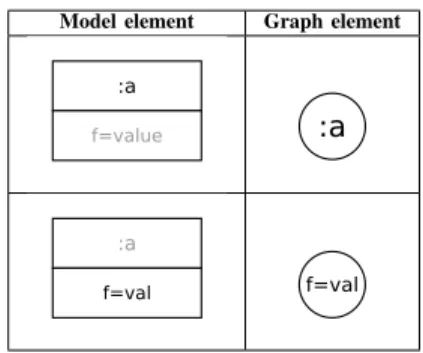
1) From models to graphs: Centrality functions are defined
on graphs, and models could be considered as labelled and typed graphs. Our graph representation of models is obtained as follows:
• Create a node for each class instance (central nodes).
• Create a node for each attribute (leaf nodes).
• Create an edge from each class instance to its attributes.
• Create an edge for each simple reference between two
class instances.
• Create two edges if two class instances are related by two
opposite references.
• Create an edge for each composition link.
Tables III and IV summarize and illustrate these transfor-mations rules. Real numbers c, r and t represent the weights assigned to composition links, reference links and attributes.
TABLE III. NODES TRANSFORMATION RULES.
Model element Graph element
TABLE IV. EDGES TRANSFORMATION RULES.
Model element Graph element
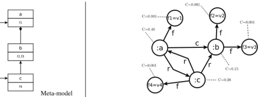
2) Centrality measure: Our centrality is inspired from
pagerank centrality and adapted to models, taking into
ac-count class instances and their attributes, links between classes (input and output) and types of link between two classes (simple references, two opposite references or compositions). For a given node v of the graph, we denote by N(v) the set of its neighbors. The following function gives the centrality of each node v:
C(v) =
∑
u∈N+(v)
C(u)
deg(u)× w(v, u).
w(v, u) gives the weight of the link between node v and u, determined by the kind of link between them (attribute, reference or composition). The weight of a link can be given by the user or deduced from domain-based quality metrics. For instance, Kollmann and Gogolla [37] described a method for creating weighted graphs for UML diagrams using object-oriented metrics.
3) Centrality vector: The centrality vector C contains the
values of centrality for each node. The previous centrality function induces the creation of a system of n variables
Meta-model
Fig. 12. Centrality vector computed for an example model and its equivalent graph.
To compute the centrality vector C we must find the eigenvector of a matrix A whose values are the coefficients of
the previous equations: C= AC, where A is built as follows:
Ai j= 0 if(vi, vj) /∈ Graph, w(vi, vj) N(vi) otherwise.
After building matrix A, we use the classical algorithm of power iteration (also known as Richard Von Mises method [38]) to compute the centrality vector C.
The result centrality vector has a high dimension (see example on Figure 12). To reduce this dimension therefore improve the computation’s efficiency, we group its coefficients according to the classes of the meta-model. Then the dimen-sion equals to the number of classes in the meta-model.
4) Centrality distance: Roy et al. proved in [39] that a
centrality measure can be used to create a graph distance. Here,
the centrality vectors CA and CB of two models A and B are
compared using any mathematical norm: d(A, B) = ||CA−CB||.
C. Discussion
We use in previous paragraphs representations of models, which could be discussed. Indeed, there are potentially many ways to vectorize models, and we choose one highly com-patible with our tool. Since CSP generation already provides a list of classes attributes and links, we simply used this representation as entry for the metrics. Again, transforming models into graphs and trees may be done through several ways. We arbitrarily choose one way that seemed to capture the graph structure. Our goal here, was to test different and diversified manners to represent a model and proposed some distance between them, not to make an exhaustive comparison study between quality of representation versus metrics. This study will be done in future works.
VII. HANDLING SETS OF MODELS
In this section, we propose an automated process for han-dling model sets. The purpose is to provide solutions for comparing models belonging to a set, selecting the most representative models in a set and bringing a graphical view of the concept of diversity in a model set.
This process helps a user in choosing a reasonable amount of models to perform his experiments (e.g., testing a model transformation). Moreover, using our approach, the chosen model set aims to achieve a good coverage of the meta-model’s solutions space.
If there are no available models, a first set of models is
generated using
G
R RIMM tool [9]. These generated modelsare conform to an input meta-model and respect its OCL constraints. When probability distributions related to domain-specific metrics are added to the process, intra-model diversity is improved. Our goal is to check the coverage of the meta-model’s solutions space. In other words, we want to help a user to answer these questions: (1) how to quantify the inter-model diversity? (2) Are all these models useful and representative? (3) Which one of my model sets is the most diverse? A. Comparison of model sets
Distance metrics proposed in Section VI compare two models. To compare a set of models, we have to compute pair-wise distances between models inside the set. A symmetrical distance matrix is then created and used to quantify the inter-model diversity. It is noticeable that, thanks to the modularity of the approach, this step can be replaced by any kind of dataset production. For instance, if the user already has a set of models, it is possible to use it instead of the generated one. Moreover, another distance metric can be used instead of the metrics we propose.
B. Selecting most representative models
Our idea is that when a user owns a certain number of models (real ones or generated ones), there are some of them, which are representative. Only these models should be used in some kind of tests (e.g., robustness or performance). Most of other models are close to these representative models.
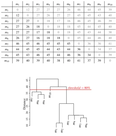
We use Hierarchical Matrix clustering techniques to select the most representative models among a set of models. The distance matrix is clustered and our tool chooses a certain number of models. In our tool, we use the hierarchical clus-tering algorithm [40], implemented in the R software (hclust, stats package, version 3.4.0) [41]. This algorithm starts by finding a tree of clusters for the selected distance matrix as shown in Figure 13. Then, the user has to give a threshold value in order to find the appropriate value. This value depends
on the diversity the user wants. For example, if the user wants models sharing only 10% of common elements, then 90% is the appropriate threshold value. This value depends also on the used metric. Thus, Levenshtein distance compares the names of elements and the values of attributes, leading to choose a smaller threshold value (for the same model set) than for centrality distance, which compares only the graph structure of the models.
Using the clusters tree and the threshold value, it is easy to derive the clusters, by cutting the tree at the appropriate height (Figure 13). The most representative models are chosen by arbitrarily picking up one model per cluster. For instance, 3 different clusters are found using the tree of clusters in Figure 13. Clone detection can also be performed using our approach by choosing the appropriate threshold value. Indeed, if threshold equals to 0, clusters will contain only clones.
TABLE V. AN EXAMPLE OF DISTANCE MATRIX (HAMMING) FOR 10 MODELS. m1 m2 m3 m4 m5 m6 m7 m8 m9 m10 m1 0 12 27 27 27 26 46 44 45 39 m2 12 0 27 26 27 27 45 45 43 40 m3 27 27 0 18 17 16 46 45 46 39 m4 27 26 18 0 18 18 45 44 45 40 m5 27 27 17 18 0 18 45 43 44 38 m6 26 27 16 18 18 0 45 44 46 40 m7 46 45 46 45 45 45 0 36 36 41 m8 44 45 45 44 43 44 36 0 34 37 m9 45 43 46 45 44 46 36 34 0 39 m10 39 40 39 40 38 40 41 37 39 0 m7 m8 m9 m10 m1 m2 m5 m4 m3 m6 10 15 20 25 30 35 40 45 Distance threshold= 80%
Fig. 13. Clustering tree computed form matrix in Table V.
C. Graphical view of diversity
Estimating diversity of model sets is interesting for model users. It may give an estimation on the number of models needed for their tests or experiments and they can use this diversity measure to compare between two sets of models.
When the number of models in a set is small, diversity can be done manually by checking the distance matrix. Unfortu-nately, it becomes infeasible when the set contains more than
an handful of models. We propose a human-readable graphical representation of diversity and solutions’ space coverage for a set of models. m1m2 m3 m4 m5 m6 m7 m8 m9 m10
Fig. 14. Voronoi diagram for 10 models compared using Hamming distance.
Our tool creates Voronoi tessellations [42] of the distance matrix in order to assist users in estimating the diversity or in comparing two model sets. A Voronoi diagram is a 2D representation of elements according to a comparison criterion, here distances metrics between models. It faithfully reproduces the coverage of meta-model’s solutions space by the set of models. Figure 14 shows the Voronoi diagram created for the matrix in Table V. The three clusters found in the previous step are highlighted by red lines. We use the Voronoi functions of R software (available in package tripack, v1.3-8).
VIII. TOOLING
This section details the tooling implementing our contri-butions. All the algorithms and tools are in free access and available on our web pages [43].
Our tool for comparing models and handling model sets
is called COMODI (COunting MOdel DIfferences). It consists
in two different parts. The first one, written in java, is used to measure differences between two models using the above 4 metrics. The second part, written in bash and R, provides algorithms for handling model sets (comparison, diversity estimation and clustering).
A. Comparing two models
It is possible to measure the differences between two models
using COMODI. For that you just need to give as input two
models and their ecore meta-model. Out tool supports two
different formats: dot model files produced by
G
RIMM andxmimodel files. COMODI supports all xmi files produced by
EMF of generated by
G
RIMM, EMF2CSP orPRAMANAtools.The first step is to parse the input models into the ap-propriate representation (graph or vector). Then, the above
distance algorithms are applied. COMODI outputs different
model comparison metrics in command line mode. Process of COMODI is described in Figure 15.
B. Handling a set of models
Our tool is also able to handle sets of models and produce distance matrices, perform clustering and plot diagrams and
Meta-model Model 1 Model 2
Xmi or dot parsers
Levenshtein distance Hamming distance
Cosine distance Centrality distance
Fig. 15. Comparing two models usingCOMODItool.
give some statistics. The input of the tool is a folder containing the models to compare and their ecore meta-model. The supported formats for models are the same as described above (xmi and dot).
Meta-model xmi or dot models Parsing models 1 Measuring differences 2
Representative Model selection
3 7 89 10 12 54 36 10 15 20 25 30 35 40 45 threshold=80%
Diversity Graphical view
4 m1m2 m3 m4 m5 m6 m7 m8 m9 m10
Fig. 16. Handling a set of models usingCOMODItool.
After parsing all the models into the appropriate repre-sentation for each metric, distance matrices are produced by pairwise comparison of models. R scripts are called to perform hierarchical clustering on these matrices. This allows us to select the most representative models of that folder. Voronoi diagrams are plotted and can be used to estimate the coverage of the folder and to compare the diversity of two folders.
COMODIprints also some simple statistics on models: closest models, most different models, etc. These steps are shown in Figure 16.
IX. APPLICATION: IMPROVING DIVERSITY
The main contributions of this paper - distances between models, representative model selection to improve diversity -were used in a work in bioinformatics (named scaffolding)
[44]. A genetic approach is paired with
G
R RIMMmodelgen-eration tool to improve the diversity of a set of automatically generated models. Figure 17 shows how we start from a
G
RIMM model set (left) with few difference between them,to
G
R RIMM (center) with a better distribution due to the probability sampler, to something very relevant by using a genetic approach (right) based on these model distances in order to improve diversity.We want to address the following question: do proposed distances and process of automated models selection help to improve the diversity and the coverage of generated models. We chose one meta-model (Figure 7) modeling a type of
graphs involved in the production of whole genomes from new-generation sequencing data [29]. Hereinafter, we give the experimental protocol:
• Generate 100 initial models conforming to the scaffold
graph meta-model using
G
R RIMM tool [9].• Model the problem of improving diversity using genetic
algorithms (GA). Our modeling in GA can be found in [11].
• Run 500 times the genetic algorithm. At each step, use
model distances and automatic model selection to choose only the best models for the next step.
• View final results in terms of model distances and
meta-model coverage using Voronoi diagrams.
The whole process induces the creation of up to 50, 000 different models. Each following figures required about 3h CP to be computed.
Curves on Figure 18 show the evolution of hamming and cosine distance while the genetic algorithm is running (minimum, maximum and mean distance over the population at each generation). We can observe that both cosine distance and hamming distance help to improve diversity of generated models. The quick convergence of both curves (around 100 iterations of GA) is a good way to check the efficiency of both models distances. We observe that the worst case in the final population is better than the best case in the initial population, thus we reached a diversity level that we did not obtained in
the initial population obtained with
G
R RIMM.We introduce several improvements to describe the fitness function used in genetic selection [11] and improve median value for final population from 0.7 up to 0.9 for Hamming and from 0.11 to 0.15 for maximum with Cosinus distance. Figure 19 compares the models produced by the different distances. Red (resp. blue) dotplots represent the distribution of distances on the final population computed using Hamming distance (resp. Cosine distance). On the left, models are compared using Hamming distance, on the right, they are compared using Cosine distance. We remark that different distances do not produce the same final models. Indeed, we can observe that the best selected models for Hamming distance obtain lower scores when compared using Cosine distance, and vice versa. Other experimental results show that our four model distances can be used in a multi-objective genetic algorithm since they treat different constructions of the meta-model. Results are better on the final model set in terms of diversity and coverage, than when only one kind of distance is used.
Figure 20 shows two Voronoi diagrams of 100 models. The first one is computed on the initial set of models, the second
on the set of models generated after the 500th iteration of
the genetic algorithm. We kept the same scale to visualize the introduced seclusion. Here we can see the insufficient solutions’ space coverage of the first Voronoi diagram. After running the multi-objective genetic algorithm, we observe a better coverage of the space. At the end of the process, we obtain 100 very distinct models.
Fig. 17. Diversity improving process. Black circles are the most representative models of the set. 0 100 200 300 400 500 0 2 · 10−2 4 · 10−2 6 · 10−2 8 · 10−2 0.1 0.12
Genetic Algorithm step
Cosine distan ce 0 100 200 300 400 500 0 0.2 0.4 0.6 0.8 1
Genetic Algorithm step
Hamming
distance
Fig. 18. Minimum, average and maximum hamming and cosine distance while running the genetic algorithm.
Fig. 19. Comparison of best selected models pairwise distances distributions.
X. CONCLUSION
This paper gathers contributions developed, in order to
complete a project (tool and methodology) named
G
RIMM(
G
eneRating Instances of Meta-Models). The topic of thesecontributions is improving the inherent quality of automati-cally generated models. We investigated the relation between the quality of the generated models and the concept of diver-sity. Our claim is that increasing the diversity when generating models, will improve their quality and usefulness, because generated models are becoming closer to real models.
We distinguish two different aspects of diversity, which are solved separately: intra-model diversity and inter-model diversity.
A. Intra-model diversity
The goal of intra-model diversity is to enrich the diversity inside a model. It is obtained by injecting randomness during the generation process. Element naming, linking objects be-come less systematic and naive. Obtained models are closer to real models, i.e., meaningful. We propose to use probability distributions, that are related to domain-specific quality met-rics. Parameters for probability laws can be chosen by users,
Fig. 20. Solutions’ space coverage of the initial set of models (left) compared to the last iteration (500th) of the genetic algorithm (right).
but they are preferably gathered by a statistical study of real data. Domain knowledge is also used when real data is rare.
We observed a substantial improvement of meaningfulness when simulated probabilities samples are added to the model generator. New generated instances have characteristics very close to real models, improving their usefulness for testing programs. This is especially interesting when data is rare, difficult or expensive to obtain, as for scaffold graphs. B. Inter-model diversity
Inter-model diversity tries to maximize the diversity of a set of models. The idea is to cover as much area in solutions’ space as possible, in order to get the best diversity ever. In our work, we propose to use model comparison and then genetic algorithm to achieve this goal.
Counting model differences is a recurrent problem in Model Driven Engineering, mainly when sets of models have to be compared. This paper tackles the issue of comparing two models using several kinds of distance metrics inspired from distances on words and distances on graphs. An approach and a tool are proposed to handle sets of models. Distance metrics are applied to those sets. Pair of models are compared and a matrix is produced. We use hierarchical clustering algorithms to gather the closest models and put them in subsets. Our tool,
COMODI, is also able to choose the most representative models of a set and give some statistics on a set of models. Human readable graphical views are also generated to help users in doing that selection manually.
First, sets of non-diverse models are automatically generated
using, for example,
G
RIMM tool. Then, COMODI is coupledto a genetic algorithm to improve the diversity of this first set of models.
C. Future work
One interesting future improvement to
G
RIMMis to becomea tool for assisting model designers, by giving quick and graphically viewable feedback during the design process. At the moment, it generates models that are close to real ones and graphical visualization is possible. Nevertheless, error detection is still poor, and it is a restriction for a large diffusion. Currently, we work on improving the interaction between the tool and the user. New features are added to the process of model generation in order to detect instantiation failures, and to correct them, or to help the user to do the correction. Guiding the user is done by interpreting the output of the CSP solver to understand the origin of any faced problem.
D. Application
The problematic of handling sets of models and the notion of distance is also involved in many other works related to testing model transformations. All these issues are interesting applications to the contributions of this paper. For example,
Mottu et al. in [45] describe a method for discovering model
transformations pre-conditions, by generating test models. A first set of test models is automatically generated, and used to execute a model transformation. Excerpts of models that make the model transformation failing are extracted. An expert then tries manually and iteratively to discover pre-conditions using these excerpts. Our common work aims to help the expert by reducing the number of models excerpts and the number of iterations to discover most of pre-conditions. A set
of models excerpts is handled using COMODI and clusters of
close models are generated. Using our method, the expert can find many pre-conditions in one iteration and using less model excerpts.
REFERENCES
[1] A. Ferdjoukh, F. Galinier, E. Bourreau, A. Chateau, and C. Nebut, “Measuring Differences To Compare Sets of Models and Improve Diversity in MDE,” in ICSEA, International Conference on Software Engineering Advances, 2017, pp. 73–81.
[2] A. Ferdjoukh, A.-E. Baert, A. Chateau, R. Coletta, and C. Nebut, “A CSP Approach for Metamodel Instantiation,” in IEEE ICTAI, 2013, pp. 1044–1051.
[3] S. Sen, B. Baudry, and J.-M. Mottu, “Automatic Model Generation Strategies for Model Transformation Testing,” in ICMT, International Conference on Model Transformation, 2009, pp. 148–164.
[4] C. A. Gonz´alez P´erez, F. Buettner, R. Claris´o, and J. Cabot, “EMFtoCSP: A Tool for the Lightweight Verification of EMF Models,” in FormSERA, Formal Methods in Software Engineering, 2012, pp. 44–50.
[5] F. Hilken, M. Gogolla, L. Burgue˜no, and A. Vallecillo, “Testing models and model transformations using classifying terms,” Software & Systems Modeling, pp. 1–28, 2016.
[6] D. S. Kolovos, D. Di Ruscio, A. Pierantonio, and R. F. Paige, “Different models for model matching: An analysis of approaches to support model differencing,” in CVSM@ICSE, 2009, pp. 1–6.
[7] D. Steinberg, F. Budinsky, M. Paternostro, and E. Merks, EMF: Eclipse Modeling Framework 2.0. Addison-Wesley Professional, 2009. [8] A. Ferdjoukh, A.-E. Baert, E. Bourreau, A. Chateau, and C. Nebut,
“Instantiation of Meta-models Constrained with OCL: a CSP Approach,” in MODELSWARD, 2015, pp. 213–222.
[9] A. Ferdjoukh, E. Bourreau, A. Chateau, and C. Nebut, “A Model-Driven Approach to Generate Relevant and Realistic Datasets,” in SEKE, 2016, pp. 105–109.
[10] F. Rossi, P. Van Beek, and T. Walsh, Eds., Handbook of Constraint Programming. Elsevier Science Publishers, 2006.
[11] F. Galinier, E. Bourreau, A. Chateau, A. Ferdjoukh, and C. Nebut, “Genetic Algorithm to Improve Diversity in MDE,” in META, 2016, pp. 170–173.
[12] J. Cabot, R. Claris´o, and D. Riera, “Verification of UML/OCL Class Di-agrams using Constraint Programming,” in ICSTW, IEEE International Conference on Software Testing Verification and Validation Workshop, 2008, pp. 73–80.
[13] A. Mougenot, A. Darrasse, X. Blanc, and M. Soria, “Uniform Random Generation of Huge Metamodel Instances,” in ECMDA, European Con-ference on Model-Driven Architecture Foundations and Applications, 2009, pp. 130–145.
[14] H. Wu, “An SMT-based Approach for Generating Coverage Oriented Metamodel Instances,” IJISMD, International Journal of Information System Modeling and Design, vol. 7, no. 3, pp. 23–50, 2016. [15] K. Ehrig, J. K¨uster, and G. Taentzer, “Generating Instance Models from
Meta models,” SoSyM, Software and Systems Modeling, pp. 479–500, 2009.
[16] Voigt, Konrad, “Structural Graph-based Metamodel Matching,” Ph.D. dissertation, Dresden University, 2011.
[17] J.-R. Falleri, M. Huchard, M. Lafourcade, and C. Nebut, “Metamodel matching for automatic model transformation generation,” in MODELS, 2008, pp. 326–340.
[18] S. Melnik, H. Garcia-Molina, and E. Rahm, “Similarity flooding: A ver-satile graph matching algorithm and its application to schema matching,” in ICDE, 2002, pp. 117–128.
[19] K. Voigt and T. Heinze, “Metamodel matching based on planar graph edit distance,” in Theory and Practice of Model Transformations, 2010, pp. 245–259.
[20] J. Cadavid, B. Baudry, and H. Sahraoui, “Searching the Boundaries of a Modeling Space to Test Metamodels,” in IEEE ICST, 2012, pp. 131–140. [21] E. Batot and H. Sahraoui, “A Generic Framework for Model-set Se-lection for the Unification of Testing and Learning MDE Tasks,” in MODELS, 2016, pp. 374–384.
[22] S. Sen, B. Baudry, and J.-M. Mottu, “On Combining Multi-formalism Knowledge to Select Models for Model Transformation Testing,” in ICST, IEEE International Conference on Software Testing, Verification and Validation, 2008, pp. 328–337.
[23] B. Henderson-Sellers, Object-Oriented Metrics: Measures of Complex-ity. Prentice Hall, 1996.
[24] E. Van Emden and L. Moonen, “Java quality assurance by detecting code smells,” in Conference on Reverse Engineering. IEEE, 2002, pp. 97–106.
[25] M. Mitzenmacher and E. Upfal, Probability and Computing: Random-ized Algorithms and Probabilistic Analysis. Cambridge University Press, 2005.
[26] “Qualitas corpus,” qualitascorpus.com/docs/catalogue/20130901/index.html, accessed: 2018-05-29.
[27] “Metrics tool,” metrics.sourceforge.net, accessed: 2018-05-29. [28] “R software,” www.r-project.org, accessed: 2018-05-29.
[29] M. Weller, A. Chateau, and R. Giroudeau, “Exact approaches for scaffolding,” BMC Bioinformatics, vol. 16, no. 14, pp. 1471–2105, 2015. [30] C. Brun and A. Pierantonio, “Model differences in the eclipse modeling framework,” UPGRADE, The European Journal for the Informatics Professional, vol. 9, no. 2, pp. 29–34, 2008.
[31] G. Sz´arnyas, Z. Kov´ari, ´A. Sal´anki, and D. Varr´o, “Towards the char-acterization of realistic models: evaluation of multidisciplinary graph metrics,” in MODELS, 2016, pp. 87–94.
[32] R. W. Hamming, “Error detecting and error correcting codes,” Bell System technical journal, vol. 29, no. 2, pp. 147–160, 1950.
[33] A. Singhal, “Modern information retrieval: A brief overview,” IEEE Data Engineering Bulletin, vol. 24, no. 4, pp. 35–43, 2001.
[34] V. Levenshtein, “Binary codes capable of correcting deletions, insertions, and reversals,” in Soviet physics doklady, vol. 10, no. 8, 1966, pp. 707– 710.
[35] G. Kishi, “On centrality functions of a graph,” in Graph Theory and Algorithms. Springer, 1981, pp. 45–52.
[36] L. Page, S. Brin, R. Motwani, and T. Winograd, “The PageRank citation ranking: bringing order to the web,” Stanford InfoLab, Tech. Rep., 1999. [37] R. Kollmann and M. Gogolla, “Metric-based selective representation of
uml diagrams,” in CSMR. IEEE, 2002, pp. 89–98.
[38] R. von Mises and H. Pollaczek-Geiringer, “Praktische verfahren der gleichungsaufl¨osung.” ZAMM-Journal of Applied Mathematics and Me-chanics, vol. 9, no. 2, pp. 152–164, 1929.
[39] M. Roy, S. Schmid, and G. Tr´edan, “Modeling and measuring Graph Similarity: the Case for Centrality Distance,” in FOMC, 2014, pp. 47– 52.
[40] F. Murtagh, “Multidimensional clustering algorithms,” Compstat Lec-tures, Vienna: Physika Verlag, 1985, 1985.
[41] R Development Core Team, R: A Language and Environment for Statistical Computing, R Foundation for Statistical Computing, 2008. [42] F. Aurenhammer, “Voronoi diagrams a survey of a fundamental
geo-metric data structure,” CSUR, ACM Computing Surveys, vol. 23, no. 3, pp. 345–405, 1991.
[43] “Download comodi,” github.com/ferdjoukh/comodi, accessed: 2018-05-29.
[44] C. Dallard, M. Weller, A. Chateau, and R. Giroudeau, “Instance guar-anteed ratio on greedy heuristic for genome scaffolding,” in COCOA, Combinatorial Optimization and Applications, 2016, pp. 294–308. [45] J.-M. Mottu, S. Sen, J. Cadavid, and B. Baudry, “Discovering model
transformation pre-conditions using automatically generated test mod-els,” in ISSRE, International Symposium on Software Reliability Engi-neering, 2015, pp. 88–99.
View publication stats View publication stats