J. Sjolte5,**
1UJF – Grenoble 1/CNRS, Laboratoire de Glaciologie et G´eophysique de l’Environnement (LGGE) UMR 5183, Grenoble, 38041, France
2Laboratoire des Sciences du Climat et de l’Environnement (LSCE)/IPSL, CEA-CNRS-UVSQ, UMR 8212, 91191 Gif-sur-Yvette, France
3D´epartement de G´eographie, Universit´e de Li`ege, Li`ege, Belgium 4CNRM-GAME, URA CNRS-M´et´eo-France 1357, Toulouse, France 5Center for Ice and Climate, Niels Bohr Institute, Copenhagen, Denmark
*now at: Institute for Meteorology and Climate Research, Karlsruhe Institute of Technology, Karlsruhe, Germany **now at: GeoBiosphere Science Centre, Quaternary Sciences, Lund University, S¨olvegatan 12, 223 62 Lund, Sweden
Correspondence to: A. Quiquet ([email protected])
Received: 13 February 2012 – Published in The Cryosphere Discuss.: 15 March 2012 Revised: 19 July 2012 – Accepted: 1 August 2012 – Published: 18 September 2012
Abstract. Predicting the climate for the future and how it
will impact ice sheet evolution requires coupling ice sheet models with climate models. However, before we attempt to develop a realistic coupled setup, we propose, in this study, to first analyse the impact of a model simulated climate on an ice sheet. We undertake this exercise for a set of regional and global climate models. Modelled near surface air temperature and precipitation are provided as upper boundary conditions to the GRISLI (GRenoble Ice Shelf and Land Ice model) hy-brid ice sheet model (ISM) in its Greenland configuration.
After 20 kyrs of simulation, the resulting ice sheets high-light the differences between the climate models. While modelled ice sheet sizes are generally comparable to the ob-served one, there are considerable deviations among the ice sheets on regional scales. These deviations can be explained by biases in temperature and precipitation near the coast. This is especially true in the case of global models. But the deviations between the climate models are also due to the dif-ferences in the atmospheric general circulation. To account for these differences in the context of coupling ice sheet mod-els with climate modmod-els, we conclude that appropriate down-scaling methods will be needed. In some cases, systematic corrections of the climatic variables at the interface may be required to obtain realistic results for the Greenland ice sheet (GIS).
1 Introduction
Recent growing awareness of the possible consequences of global warming on ice sheets (4th assessment report of the Intergovernmental Panel on climate change, IPCC-AR4, Meehl et al., 2007) has led to the developing of numerical models aiming to predict their future evolution. While esti-mates of surface mass balance (SMB) from climate models give insights into the response of the ice sheet surface to cli-mate warming (e.g., Yoshimori and Abe-Ouchi, 2012), ice sheet models (ISMs) must also be used to simulate the long-term evolution of ice sheets (e.g., Robinson et al., 2010). At the same time, awareness of the importance of feedback from other components of the Earth system has risen and sev-eral attempts have been undertaken to integrate ISMs into climate models in order to include and evaluate these feed-back mechanisms for the upcoming centuries (Ridley et al., 2005; Vizca´ıno et al., 2008, 2010). These feedbacks include, for example, water fluxes to the ocean (Swingedouw et al., 2008), orography variations (Kageyama and Valdes, 2000) and albedo changes (Kageyama et al., 2004).
However, when model results are compared with actual observations, major uncertainties remain due to shortcom-ings in both climate models and ISMs. Because of the long time scales involved in ice sheet development, synchronous
coupling is feasible only with low resolution and physi-cally simplified earth system models (e.g., Fyke et al., 2011; Driesschaert et al., 2007). Direct synchronous coupling with a fine resolution using a physically sophisticated atmospheric general circulation model (GCM) is still a challenge (Pol-lard, 2010). Recent approaches try to avoid this problem by implementing asynchronous coupling of the climate models and ISMs (Ridley et al., 2010; Helsen et al., 2012).
The recent observations of fast processes at work in the Greenland and West Antarctic ice sheets (e.g., Joughin et al., 2010) show the need for synchronous coupling between the ISMs that represent these processes and coupled atmosphere-ocean GCMs (AOGCMs) if we want to predict the state of the ice sheets in the near future, i.e., the coming century. The ISMs should include fast processes such as fast flow-ing ice streams and groundflow-ing line migration. These ISMs are becoming available (Ritz et al., 2001; Bueler and Brown, 2009) and the first step towards their coupling to GCMs is to examine how they perform when forced by the GCM out-puts. Until recently, the major concern of ISM developers was to improve the representation of physical processes oc-curring inside or at the boundaries of the ice sheet (e.g., Ritz et al., 1997; Tarasov and Peltier, 2002; Stone et al., 2010), primarily in order to better simulate past ice sheet evolu-tion. In reconstructions of the paleo-climate, ISMs are often forced by ice core-derived proxy records, with spatial reso-lution of atmospheric conditions stemming from reanalysis (e.g., Bintanja et al., 2002), or from climate model snapshots (Letr´eguilly et al., 1991; Greve, 1997; Tarasov and Peltier, 2002; Charbit et al., 2007; Graversen et al., 2010). But for re-liable projections of the future ice sheet state the explicit use of climate model scenarios is necessary. More specifically, the first test is to evaluate how a Greenland ISM responds when forced by output from different GCMs. Considering that the extent of the ablation zone is often less than 100 km (van den Broeke et al., 2008), the GCMs generally have a coarse resolution compared with the typical ISMs. We con-sequently need to assess the gain provided by higher resolu-tion models, such as regional climate models (RCMs), even if the trade off is a more limited scope.
To date, few studies have tested the sensitivity of an ISM to atmospheric forcing fields explicitly. Charbit et al. (2007) showed that an ISM forced by six GCMs simulations from the Paleo Climate Intercomparison Project (PMIP) was un-able to reproduce the last deglaciation of the Northern Hemi-sphere. They showed great discrepancies between the six simulated ice volume evolutions. The fast processes men-tioned earlier were not included in this study because the ISM they used does not include ice streams representation. Graversen et al. (2010) simulated the total sea level in-crease over the next century using the GCMs from the Cou-pled Model Intercomparison Project phase 3 (CMIP-3). Here again, the ISM they used does not take into account the ice streams. Although different climate model outputs were used as forcing fields, neither the studies mentioned above, nor the
parameter-based approaches (e.g., Hebeler et al., 2008; Stone et al., 2010), illustrate directly the links between climate forc-ing and simulated ice sheet behaviour. That is the main goal of the present study.
We present and discuss some of the difficulties arising when combining ice sheet and climate models. We restrict our study to the case of Greenland and choose an uncoupled approach: to examine the sensitivity of a single state-of-the-art Greenland ice sheet (GIS) model to atmospheric input fields stemming from a number of selected climate models. Then, for comparison and in the tradition of previous ISM studies, we examine a reference case derived from meteoro-logical observations.
In Sect. 2, we first present our state-of-the-art ISM and its specifications. We then explain how we selected the climate models with different degrees of resolution and comprehen-siveness. The downscaling of atmospheric variables and the SMB computation is then described. Finally, we discuss how we calibrated the ISM and set it up for the sensitivity ex-periments. The results of the ISM simulations are shown in Sect. 3. The links between the climate model biases and horizontal resolution on the one hand, and simulated devi-ations in ice sheet size and shape on the other hand are dis-cussed. Our conclusions and suggestions for future directions to explore in climate-ice sheet model studies are presented in Sect. 4.
2 Tools and methodology 2.1 The GRISLI ice sheet model
The model used here is a three-dimensional thermo-mechanically coupled ISM called GRISLI. With respect to ice flow dynamics, it belongs to the hybrid model type: it includes both the shallow ice approximation (SIA, Hutter, 1983) and the shallow shelf approximation (SSA, MacAyeal, 1989) to solve the Navier-Stokes equations. This model has been validated on the Antarctic ice sheet (Ritz et al., 2001; Philippon et al., 2006; ´Alvarez-Solas et al., 2011a) and has been successfully applied on the northern hemisphere ice sheets for paleo-climate experiments (Peyaud et al., 2007;
´
Alvarez-Solas et al., 2011b). In the more recent version used here, the combination of SIA and SSA is the following:
1. A map of “allowed” ice streams is determined on the basis of basal topography. More specifically, we as-sume that ice streams are located in the bedrock val-leys (Stokes and Clark, 1999). These valval-leys are derived from the difference between bedrock elevation at any given grid point and bedrock elevation smoothed over a 200-km radius around this point. Additionally, ice streams are allowed where observed present-day veloc-ities (Joughin et al., 2010) are greater than 100 m yr−1 even if the bedrock criterion is not fulfilled.
grounded ice flow is computed using the SIA only. Ice shelves are processed with SSA only.
Calving is parameterised with a simple cut-off based on a threshold on the ice thickness. This threshold is spatially uniform but time-dependent. Its value varies with the surface temperature anomaly used in the spin-up experiment pre-sented in Sect. 2.4.1. For the present climate, the threshold is 250 m.
One of the features of the GRISLI model is a polynomial constitutive equation, that combines the strain rate compo-nents from Glen and Newtonian flow laws. This kind of law, already used in Ritz et al. (1983), accounts for the fact that the exponent of the flow law depends on the stress range (Lliboutry and Duval, 1985). Additionally, as in most large scale ISMs, we use enhancement factors that are multipli-cation coefficients supposed to represent the impact of ice anisotropy on deformation. According to Ma et al. (2010), enhancement factors are different for SIA and SSA because the impact on the rate of deformation of the fabric, typi-cally with a vertitypi-cally oriented C-axis, depends on the stress regime. We, thus, have four different enhancement factors, one for each component of the flow law (Newtonian or Glen) and for SIA and SSA (here called E1SIA and E3SIA for SIA Newtonian and Glen, respectively, and E1SSA and E3SSA for SSA Newtonian and Glen, respectively). These factors are not completely independent because the stronger a factor is for SIA, the smaller it is for SSA. These four enhancement factors are tuned during the dynamic calibration procedure (see Sect. 2.4.1 below and Table 1 for the values).
The model is run on a 15-km Cartesian grid resulting from the stereographic projection with the standard parallel at 71◦N and the central meridian at 39 ◦W. The bedrock
elevation map comes from the ETOPO1 dataset, which it-self combines other maps (Amante and Eakins, 2009). The ice sheet thickness map is derived from the work of Bamber et al. (2001). The surface elevation is the sum of the bedrock elevation and ice thickness. Figure 1 presents the initial to-pography, which is also referred to as the observed topog-raphy. Note that under this construction there are no floating points at the time of initialisation. We use the geothermal heat flux distribution proposed by Shapiro and Ritzwoller (2004).
Fig. 1. Present day topography of the GIS, used to initialise the ISM. Selected weather stations are represented.
figure
39
Fig. 1. Present day topography of the GIS, used to initialise the ISM.
Selected weather stations are represented.
The procedure to initialise the thermal state of the ice sheet is described in Sect. 2.4.
2.2 Atmospheric model forcing fields
The ISM requires the climatological monthly mean values for the near surface air temperature and precipitation as well as the surface topography for the corresponding atmospheric forcings. These are derived from a common 20-year refer-ence period, 1980–1999. The length of 20 years is a com-promise between the need for meaningful climatology on the one hand and the consistency of boundary conditions used for driving the regional models and reanalysis on the other hand.
Among the CMIP-3 coupled atmosphere-ocean GCMs used for the IPCC-AR4, there are significant discrepancies regarding the Greenland climate (Franco et al., 2011; Yoshi-mori and Abe-Ouchi, 2012). We selected two models with reasonable agreement to reanalysis (Franco et al., 2011), but diverging mass balance projections, as discussed in Yoshi-mori and Abe-Ouchi (2012):
– The coupled atmosphere-ocean GCM CNRM-CM3
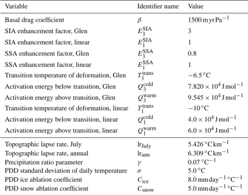
Table 1. Model parameters used in the GRISLI model for this study.
Variable Identifier name Value
Basal drag coefficient β 1500 m yr Pa−1
SIA enhancement factor, Glen ESIA3 3
SIA enhancement factor, linear ESIA1 1
SSA enhancement factor, Glen ESSA3 0.8
SSA enhancement factor, linear ESSA1 1
Transition temperature of deformation, Glen T3trans −6.5◦C
Activation energy below transition, Glen Qcold3 7.820 × 10⁴J mol−1 Activation energy above transition, Glen Qwarm3 9.545 × 10⁴J mol−1 Transition temperature of deformation, linear T1trans −10◦C
Activation energy below transition, linear Qcold1 4.0 × 10⁴J mol−1 Activation energy above transition, linear Qwarm1 6.0 × 10⁴J mol−1
Topographic lapse rate, July lrJuly 5.426◦C km−1
Topographic lapse rate, annual lrann 6.309◦C km−1
Precipitation ratio parameter γ 0.07◦C−1
PDD standard deviation of daily temperature σ 5.0◦C
PDD ice ablation coefficient Cice 8.0 mm day−1 ◦C−1
PDD snow ablation coefficient Csnow 5.0 mm day−1 ◦C−1
– The coupled atmosphere-ocean GCM IPSL-CM4
(Marti et al., 2010).
Surface climate fields were extracted from the CMIP-3 20th century transient simulations for years 1980 to 1999.
In addition, as an example of an atmosphere-only model with GCM resolution, we included the atmospheric compo-nent of the IPSL model, but in a version with an improved physical ice sheet surface scheme, as follows:
– The global atmosphere-only GCM, LMDZ, with an
ex-plicit snow model adapted from the SISVAT model, as used in the regional model MAR (Brun et al., 1992; Gall´ee et al., 2001), termed LMDZSV. Here and for the following climate models, we imposed SST and sea ice boundary conditions for the years 1980–1999. The in-troduction of a more realistic snow scheme on ice sheets makes this version of LMDZ very different from the standard one in terms of surface climate (Punge et al., 2011).
This climate forcing is meant to identify the impact of an im-proved representation of surface climate processes in a GCM on ice sheet evolution.
To study the impact of resolution in a GCM, we also con-sidered:
– The global atmosphere-only GCM LMDZ4 with an
im-proved resolution on Greenland (Krinner and Genthon, 1998; Hourdin et al., 2006), termed LMDZZ (for zoom). The much higher resolution over Greenland compared with IPSL-CM4 induces scaling effects of the parameterisations
which leads to very different surface climates. In particular, the impact of orography near the coast is much better repre-sented in the zoomed model, and it can influence moisture transport and temperature over the entire ice sheet.
Regional climate models achieve much higher spatial res-olution than GCMs, but require lateral boundary conditions. We selected:
– The regional climate model MAR (Fettweis, 2007;
Lefebre et al., 2002). The model output we used stems from the 1958–2009 simulation (Fettweis et al., 2011), forced by ERA40 as boundary conditions. We use the near surface air temperatures at 3 m provided by the MAR output, instead of 2 m temperatures used in all other cases, but this is not likely to affect our analysis significantly.
– The regional climate model REMO (Sturm et al., 2005;
Jacob and Podzun, 1997), as used in a recent isotope study on Greenland precipitation (Sjolte et al., 2011), forced by ECHAM4 as lateral boundary conditions and nudged to the upper level wind field. The ECHAM4 simulation is itself nudged towards the ERA40 wind and temperature fields every six hours. For a complete de-scription of the nudging procedure, see von Storch et al. (2000).
As for the GCMs, this selection is in no way meant to be complete. It was guided in part by the availability of the model output at the beginning of the study, but still repre-sents the state-of-the-art climate representation.
(a)
(b)
Fig. 2. Greenland (land points) mean seasonal cycle of near surface air temperature (in
◦C, left panel)
and precipitation (in millimeters of water equivalent per month, right panel) for the 8 atmospheric forcing
fields used in this study (colored lines). For FE09, temperature is representative for the 1996-2006 period
(Fausto et al., 2009) and precipitation for the 1958-2009 period (Ettema et al., 2009). For the other forcing
fields, climatological means are evaluated on the 1980-1999 period. Annual mean values are represented
by triangles on the right. The grey, shaded area is the spread of 12 CMIP-3 models. Light grey and black
lines respectively represent individual models and their means.
40
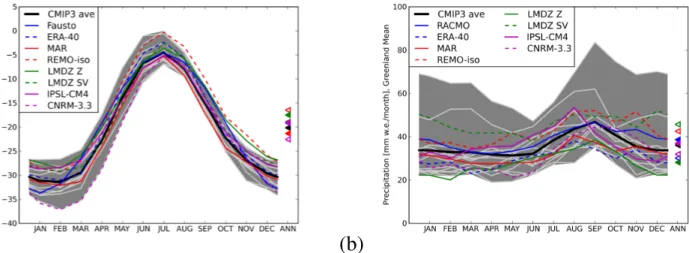
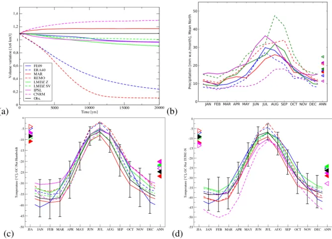
Fig. 2. Greenland (land points) mean seasonal cycle of near surface air temperature (in◦C, left panel) and precipitation (in millimetres of water equivalent per month, right panel) for the 8 atmospheric forcing fields used in this study (coloured lines). For FE09, temperature is representative for the 1996–2006 period (Fausto et al., 2009) and precipitation for the 1958–2009 period (Ettema et al., 2009). For the other forcing fields, climatological means are evaluated on the 1980–1999 period. Annual mean values are represented by triangles on the right. The grey, shaded area is the spread of 12 CMIP-3 models. Light grey and black lines, respectively, represent individual models and their means.
As an example for a reanalysis, we further used:
– The reanalysis ERA40 (Uppala et al., 2005).
Finally, in our comparison we include a composite at-mospheric field using parameterised temperature based on geographical coordinates and altitudes together with high-resolution assimilation-based precipitation fields, as fre-quently used by ice sheet modellers (e.g., Ritz et al., 1997; Greve, 2005). It consists of:
– The temperature parameterisation of Fausto et al.
(2009) and the precipitation field of the regional model RACMO2 (Ettema et al., 2009) run with ERA40 as boundary conditions over the 1958–2009 time span. We will refer to this forcing set as FE09. The FE09 atmo-spheric forcing field was distributed by the CISM com-munity and used, for example, in Greve et al. (2011). From the ice sheet modellers point of view, this forcing field may be regarded as a reference.
The different model resolutions and external forcings are summarised in Table 2.
The AOGCMs simulate atmospheric surface conditions in interaction with their ocean and sea ice components and with none or few external sources of variability. Hence, the simulated time series cannot be expected to correlate with observed variables as in the atmosphere-only models with observation-derived lower boundary conditions.
In terms of annual mean near surface air temperature and precipitation, the atmospheric forcing fields used in this study are within the range of the CMIP-3 models, but re-flect the broad dispersion, as shown in Fig. 2. We chose to use temperature and precipitation forcing fields from vari-ous models. These forcing fields are outputs from coupled
atmosphere-ocean GCMs, atmosphere-only GCMs, regional models and reanalysis. We assume that the range of uncer-tainty of CMIP-3 models is a conservative estimate of the un-certainty of observed temperature and precipitation in Green-land. Figure 2a shows that the temperature spread among the model outputs we selected is comparable to that of the CMIP-3 models. By contrast, the precipitation spread among the forcing fields we selected is smaller than that of the CMIP-3 models (Fig. 2b). Note, however, that the spread of the CMIP-3 ensemble is artificially increased by one model that probably overestimates the total amount of precipitation over Greenland.
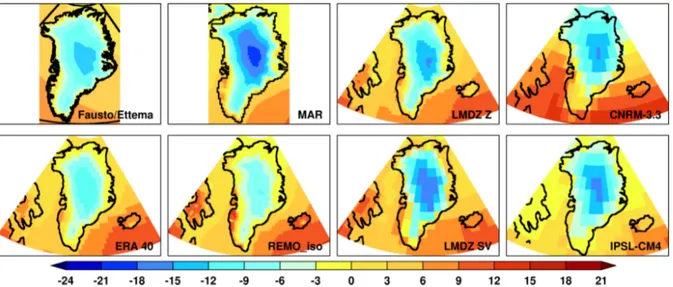
Figures 3 and 4 show the 1980–1999 climatological annual mean 2 m temperature and precipitation, respectively, on and around Greenland. On these figures, the original polar stereo-graphic grid was preserved for MAR and FE09; the results of the other models are presented on polar stereographic projec-tions. Several large scale features can be seen in Fig. 3: the MAR and CNRM models have relatively low temperatures in central and northern Greenland, while REMO is warmer than the other models on the ice sheet, and CNRM seems to be too warm on the southern part of the GIS. Even if the coarse resolution global models fail to resolve the fine pattern of the coastal high precipitation zone (Fig. 4), all the climate models simulate correctly a precipitation maximum in South-East Greenland. However, the amplitude of this maximum is too low for MAR and ERA40. CNRM is the driest model in the northern part of the GIS. Section 3 will show how these different climatic conditions, caused by different represen-tations of orography and boundary conditions, but also by different dynamical schemes and physical parameterisations, affect the simulated ice sheet.
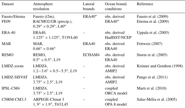
Table 2. Main characteristics of atmospheric forcing fields used for this study.
Dataset Atmosphere Lateral Ocean bound. Reference
resolution bounds conditions
Fausto/Ettema Fausto (t2m), ERA40∗ obs. derived Fausto et al. (2009)
FE09 RACMO2/GR (precip.), ERA40∗ Ettema et al. (2009)
0.29◦×0.29◦, L40∗
ERA-40 ERA40, – obs. derived Uppala et al. (2005)
1.125◦×1.125◦, T159 L60 HadISST/NCEP
MAR MAR, ERA40 obs. derived Fettweis (2007)
0.66◦×0.66◦ ERA40
REMO REMO, ECHAM4 obs. derived Sturm et al. (2005)
0.5◦×0.5◦, L19 ERA40
LMDZ-zoom LMDZ4, – obs. derived Krinner and Genthon (1998)
1.2−3.6◦×0.5−5.5◦, L19 AMIP2
LMDZ-SISVAT LMDZ4, – obs. derived Punge et al. (2011)
3.75◦×2.5◦, L19 AMIP2
IPSL-CM4 LMDZ4, – coupled Marti et al. (2010)
3.75◦×2.5◦, L19 ORCA model
CNRM-CM3.3 ARPEGE-Climat 3 – coupled Salas-M´elia et al. (2005)
1, 9◦×1.9◦, T63 L45 OPA 8 model
Resolutions in◦approximated. *: for RACMO2/GR
2.3 SMB computation
The ISM is forced by the atmospheric fields described in Sect. 2.2. To compute the SMB, we use monthly means of temperature and precipitation for present day climate. Even if the SMB is an output of the atmospheric models, we can-not use it directly for the ISM because of the large differ-ence in resolution between the two grids. Innovative tech-niques using SMB gradients exist (Helsen et al., 2012), but are strictly limited to high resolution climate models with so-phisticated snow schemes and consequently exclude GCMs. The downscaling of near surface air temperature and precip-itation is physically based, as detailed below, contrary to the SMB downscaling, which is not. Thus, we compute the SMB from downscaled temperature and precipitation means.
Ablation is computed with the widely-used Positive De-gree Days (PDD) method (Reeh, 1991). Even if this method is a very schematic representation of surface melt (van den Broeke et al., 2010), it can be tuned to simulate the observed SMB and its variability (Tarasov and Peltier, 2002; Fausto et al., 2009b), consequently it is still commonly used among the glaciologist community (e.g., Peyaud et al., 2007; Greve et al., 2011; Kirchner et al., 2011; Graversen et al., 2010). We also chose this method because it requires a limited num-ber of atmospheric fields, which are easy to obtain from the different models. We compute the number of PDD, repre-senting melt capacity, numerically at each grid point, based on the downscaled monthly mean near-surface temperature. Following Reeh (1991), a statistical temperature variation is considered, allowing melt even in months with mean
temper-ature below the freezing point. The melt capacity computed with the PDD method is first used to melt the snow layer. A fraction of the melted snow is allowed to percolate into the snowcover and refreeze, generating superimposed ice. Melt water runoff is allowed if the amount of superimposed ice reaches the limit of 60 % of the snowcover (Reeh, 1991). The refreezing is responsible for firn warming, as described in Reeh (1991). The remaining PDD are used to melt possible superimposed ice from refreezing and then old ice.
The PDD integration constants and the melt rates of snow and ice are listed in Table 1. We chose Csnowto be substan-tially higher than in Reeh (1991). But the melting rate co-efficients are poorly constrained and a wide range of values can be found in the literature (van den Broeke et al., 2010). This choice was motivated by the better agreement of ab-lation with the one simulated in regional models (Fettweis et al., 2011; Ettema et al., 2009).
The ISM distinguishes between rainfall and snowfall. Liq-uid precipitation does not contribute to the surface mass bal-ance and is assumed to run off instantaneously. This proce-dure is a drastic simplification, but still commonly employed (Charbit et al., 2007; Peyaud et al., 2007; Hubbard et al., 2009; Kirchner et al., 2011). An explicit refreezing model (Janssens and Huybrechts, 2000) was tested, but produced only slight differences (not shown). The monthly solid pre-cipitation, Psm, is calculated based on total monthly precipi-tation Pmand monthly near surface air temperature Tm, fol-lowing Marsiat (1994):
Fig. 3. Climatological (1980-1999) June-July-August mean 2 m temperature in the eight different climate
models (in
◦C).
41
Fig. 3. Climatological (1980–1999) June–July–August mean 2 m temperature in the eight different climate models (in◦C).
Fig. 4. Climatological (1980-1999) annual mean precipitation (solid + liquid) in the eight different
cli-mate models (in metres of ice equivalent).
42
Fig. 4. Climatological (1980–1999) annual mean precipitation (solid + liquid) in the eight different climate models (in metres of ice
equiva-lent). Psm Pm = 0 , Tm≥7◦C (7◦C − Tm)/17◦C , −10◦C ≥ Tm≥7◦C 1 , Tm≤ −10◦C (1)
As the ice sheet topography changes during the simula-tion, and can hence differ strongly from the one prescribed in the atmospheric models, the near surface air tempera-ture has to be adapted. For this correction, we use a verti-cal temperature gradient, referred to hereafter as topographic lapse rate, which does not vary spatially, but is different from month to month. The monthly values follow an annual si-nusoidal cycle with a minimum in July at 5.426◦C km−1and an annual mean of 6.309◦C km−1. They are derived from the
Greenland surface temperature parameterisation proposed by Fausto et al. (2009). The adaptation method is, thus, consis-tent with the FE09 reference experiment. The gradients ob-tained in this way are derived from spatial variations of near surface air temperature and not from the actual temperature response to surface elevation changes at each grid point. This information could be obtained only by repeated atmospheric model simulations with different topographies, as performed by Krinner and Genthon (1999), who found values that are close to the ones we use here. The hypothesis that the sensi-tivity of the results to topographic lapse rate is of secondary order compared to the different forcing fields is tested in Sect. 3.5.
The temperature field from the low resolution topography of the climate model (T0) is downscaled to the high resolution required for the ISM (Tref) using the topographic lapse rate correction as described above. For the downscaling of the precipitation rate, we used an empirical law that links tem-perature differences to accumulation ratio (Ritz et al., 1997):
Pref
P0
=exp(−γ × (Tref−T0)), (2)
in which the ratio of precipitation change with temperature change, γ , is poorly constrained (Charbit et al., 2002). We use a value of γ = 0.07, which corresponds to a 7.3 % change of precipitation for every 1◦C of temperature change (Huy-brechts, 2002).
We chose to use the same parameters for SMB calculations for all atmospheric forcings, because our goal is to compare the sensitivity of the ISM to the forcing, not to determine the parameters which yield the most realistic GIS for each forcing.
2.4 Experimental setup of the ice sheet model 2.4.1 Spin-up and dynamic calibration
The calibration/initialisation of an ISM is a difficult prob-lem that would require assimilation methods to be accurately solved (Arthern and Gudmundsson, 2010). In the experi-ments presented here we wanted to start from fields as close as possible to the present state. The prognostic variables of ISMs are ice thickness, bedrock topography and ice tempera-ture. The first two of them are the reasonably well-known 2-D horizontal fields (Bamber et al., 2001; Layberry and Bam-ber, 2001; Amante and Eakins, 2009). The 3-D temperature field is much more difficult to estimate, but is also crucial because it is strongly linked to the velocity distribution. The temperature distribution within the ice depends on the past evolution of the ice sheet, in particular on past boundary con-ditions including surface mass balance and near surface air temperature. The typical time scale of thermal processes is up to 20 kyrs (Huybrechts, 1994), so today’s ice temperature is still affected by the temperature increase during the last deglaciation.
To account for this past evolution, we run a long glacial-interglacial spin-up simulation to obtain a realistic present temperature field. To do so, we use present day climatic con-ditions and apply perturbations deduced from proxy data. The present day atmospheric fields of temperature and pre-cipitation are the same as in the FE09 experiment.
The temperature perturbations with respect to the present day were reconstructed following Huybrechts (2002) based on the GRIP isotopic record (Dansgaard et al., 1993; Johnsen et al., 1997), using a constant slope of 0.42 ‰◦C−1. These time-dependent and spatially uniform perturbations are used as deviations from present day conditions to force the ISM.
The resulting precipitation perturbations are assumed to fol-low the temperature evolution as in Eq. 2.
However, the 3-D temperature field obtained after this spin-up procedure corresponds to a topography that is differ-ent from the observed one. Consequdiffer-ently, for the sensitivity experiments, we stretch the temperature field to the observed topography in order to obtain the initial state.
Once the 3-D temperature field has been obtained, we tune the various parameters that govern the velocity field by per-forming dynamic calibration.
These are the four enhancement factors and the β coeffi-cient of the basal drag presented in Sect. 2.1. Assuming that after the spin-up procedure the temperature field is realistic, the velocity field will depend on these parameters only. Our target is the surface velocity field measured by radar interfer-ometry (Joughin et al., 2010).
We must stress that for ice streams, it is almost impossi-ble to tune the coefficient β of basal drag and the enhance-ment factors ESSA1 and ESSA3 separately. As explained in Sect. 2.1, the SIA and SSA enhancement factors are not in-dependent and we added a constraint on the relationship be-tween SIA and SSA. This is because the enhancement fac-tors are both equal to 1.0 in the case of isotropic ice, and the stronger the ice anisotropy, the higher the SIA enhancement factors and the lower the SSA enhancement factors (Ma et al., 2010). We chose ESSA=0.9 for ESIA=2.0, ESSA=0.8 for ESIA=3.0, and ESSA=0.63 for ESIA=5.0. The pro-cedure consists in running short (100 years) simulations in a constant present day climate. We ran a matrix of sim-ulations by varying simultaneously and independently the five parameters already mentioned: the enhancement fac-tors ESSA1 , E3SSA, E1SIA and E3SIA, and the β coefficient of basal drag. The range tested for the SIA enhancement fac-tors was 1.0 < ESIA<5.0, corresponding to SSA factors of 1.0 > ESSA>0.63. The range tested for the β coefficient was 500 to 1500 Pa.yr/m.
For each set of parameters, we computed mean squared error and standard deviation, in terms of difference between observed and simulated velocities as well as in terms of the respective flux of ice (being the velocity multiplied by the ice depth). The best set of parameters corresponds to the mini-mum values of mean squared error and standard deviation. Considering that a different set of parameters can give ap-proximately the same statistical scores, we also examined the corresponding mapped velocity amplitudes and distribution histogram and compared then with the observed velocity.
This best set obtained was with:
– Glen cubic law: ESIA3 =3.0 and ESSA3 =0.8.
– Newtonian finite viscosity: ESIA1 =1.0 and E1SSA=1.0.
– Coefficient of basal drag: β = 1500 Pa yr m−1.
These values are consistent with the findings of Ma et al. (2010), and with the range 3.0–5.0 generally used in the SIA
Fig. 5. Simulated ice sheet topography at the end of the 20-kyr constant climate forcing model run.
43
Fig. 5. Simulated ice sheet topography at the end of the 20-kyr constant climate forcing model run.
and Glen flow law case. We used this set of parameters in all further experiments.
This solution is not unique, because we can obtain the same velocity field with more viscous ice streams (lower SSA enhancement factor) and weaker basal drag. It is worth noting that our dynamical calibration is almost independent of the atmospheric forcing fields used. Ice velocity is indeed a diagnostic variable which depends on surface and bedrock topography, 3-D temperature field, basal drag and ice defor-mation properties, but it does not depend directly on surface mass balance.
Our calibration is, however, impacted by the initial tem-perature field. Temtem-perature is a prognostic variable and, thus, depends on the past ice sheet evolution, past surface tem-perature and poorly constrained distribution of geothermal heat flux (Greve, 2005). However, we estimate that this ef-fect is secondary when compared with the impact of the at-mospheric field.
Nonetheless, our sensitivity studies indicate that the model results are much more sensitive to surface mass balance than to dynamic parameters: with the FE09 forcing, a doubling of sliding (β/2) induces a 0.1 % reduction in total volume, whereas changing the FE09 forcing for the MAR forcing in-duces a 9.0 % increase in total volume.
2.4.2 Sensitivity test procedure
Having calibrated the dynamical parameters, we compare the responses with the various climate model forcings. We keep the same set of dynamic and mass balance downscaling pa-rameters in all the experiments and change only the atmo-spheric fields of total precipitation and near surface air tem-perature provided by the atmospheric models. We then run 20 kyr-long experiments to allow for the ice sheet to sta-bilise, while keeping the climate constant over time (“glacio-logical steady state”). Nevertheless, during these simula-tions, temperature and consequently precipitation, is likely to change, in relation with the elevation changes as described in Sect. 2.3. We do not expect, in this kind of experiment, to reproduce a realistic present day ice sheet because the present day GIS is the result of complex changes of temperature and precipitation during the last thousand years. We do not expect either to provide realistic projections of the future GIS state because we do not perturb the present day climate to take into account the rate of change of temperature and precipita-tion consequent to changes in concentraprecipita-tions of greenhouse gases. The idea here is to present an idealised configuration depending on a minimal number of parameters. The focus of our analysis in Sect. 3 will, thus, be on the range of relative deviation, from the present reference state obtained with the different atmospheric forcing fields.
(a)
(b)
(c)
(d)
Fig. 6. a: North Greenland (latitudes greater than 75
◦N) simulated ice volume evolution for the steady
state model runs shown in Fig. 5. The regional initial volume corresponds to the observed one. b:
Re-gional (land mask with latitudes greater than 75
◦N) monthly mean precipitation for each individual
atmospheric forcing, with annual mean values (triangles). c, d: Station climatology for, respectively,
Humboldt and Tunu-N (Steffen et al., 1996), and closest grid point near surface air temperature for each
individual atmospheric forcing, with July temperature (left hand triangles) and annual mean temperature
(right hand triangles). The black markers stand for the observations (initial regional ice volume and t2m
stations measurement). Vertical bars are standard deviations from the monthly mean in the observations
data sets. Time periods vary, depending on availability.
44
Fig. 6. (a): North Greenland (latitudes greater than 75◦N) simulated ice volume evolution for the steady state model runs shown in Fig. 5. The regional initial volume corresponds to the observed one. (b): Regional (land mask with latitudes greater than 75◦N) monthly mean precipitation for each individual atmospheric forcing, with annual mean values (triangles). (c, d): Station climatology for, respectively, Humboldt and Tunu-N (Steffen et al., 1996), and closest grid point near surface air temperature for each individual atmospheric forcing, with July temperature (left hand triangles) and annual mean temperature (right hand triangles). The black markers stand for the observations (initial regional ice volume and t2m stations measurement). Vertical bars are standard deviations from the monthly mean in the observations datasets. Time periods vary, depending on availability.
3 Results
3.1 20 kyr equilibrium simulated topographies
Figure 5 presents the impact of inter-model climate differ-ences in terms of simulated topography at the end of the run. Differences between simulated topographies and observed topography is available in the Supplement accompanying this paper. A remarkable diversity of simulated topographies is observed. At first sight, the simulated southern part of the ice sheet is more similar than the simulated northern part. In the North, at the end of the simulation, with two models (REMO and ERA40) presenting almost no ice, and at least three mod-els (CNRM, MAR, IPSL) presenting a fully covered area, the range is very broad. The surface height is also very differ-ent among the models with an approximate 7 % thickening for MAR in the interior and 8 % thinning with IPSL. In all the simulations, the ice sheet is spreading towards the South West. This common characteristic is due to the ISM’s
inabil-ity to reproduce fine scale features. The south of Greenland is indeed a very mountainous area characterised by high oro-graphic precipitation and strong slope effects, even in the ice flow dynamics. The 15-km grid is too coarse to reproduce such local effects and specific parameterisations would be needed (Marshall and Clarke, 1999).
To distinguish between the different regional behaviours, we consider three regions: a southern region with latitudes lower than 68◦N, a northern one with latitudes greater than
75◦N, and a central region in between. Specific differences
occur mainly in the north and in the south. The central region presents a more complex response and we were not able to identify well-defined specificities. Hence, we discuss mainly the results for the South and North regions. The evolution of the simulated volume for the northern and southern re-gions is presented in Figs. 6a and 7a, respectively. Except for MAR and CNRM experiments, all models simulate a de-crease of ice volume in the north. If we put aside REMO and
(c)
(d)
Fig. 7. a: South Greenland (latitudes lower than 68
◦N) simulated ice volume evolution for the steady
state model runs shown in Fig. 5. The regional initial volume corresponds to the observed one. b:
Re-gional (land mask with latitudes lower than 68
◦N) monthly mean precipitation for each individual
at-mospheric forcing, with annual mean values (triangles). c, d: Station climatology for, respectively, Nuuk
(DMI) and South Dome (Steffen et al., 1996), and closest grid point near surface air temperature for each
individual atmospheric forcing, with July temperature (left-sided triangles) and annual mean temperature
(right-sided triangles). The black markers stand for the observations (initial regional ice volume and t2m
stations measurement). Vertical bars are standard deviations from the monthly mean in the observations
data sets. Time periods vary, depending on availability.
45
Fig. 7. (a): South Greenland (latitudes lower than 68◦N) simulated ice volume evolution for the steady state model runs shown in Fig. 5. The regional initial volume corresponds to the observed one. (b): Regional (land mask with latitudes lower than 68◦N) monthly mean precipitation for each individual atmospheric forcing, with annual mean values (triangles). (c, d): Station climatology for, respectively, Nuuk (DMI) and South Dome (Steffen et al., 1996), and closest grid point near surface air temperature for each individual atmospheric forcing, with July temperature (left-sided triangles) and annual mean temperature (right-sided triangles). The black markers stand for the observations (initial regional ice volume and t2m stations measurement). Vertical bars are standard deviations from the monthly mean in the observations datasets. Time periods vary, depending on availability.
ERA40, which simulate nearly no ice in this region, the vol-ume variation ranges from –0.1 to +0.16 106km3in 20 kyrs. REMO and ERA40 present the same pattern of retreat proba-bly due to the nudging procedure (von Storch et al., 2000) of the REMO model towards the ERA40 reanalysis. The south-ern region systematically gains ice volume (Fig. 7a), and the response of the ISM is almost instantaneous, compared to typical evolution time scales, given that 50 % of the final vol-ume variation is generally achieved within a thousand years. The volume simulated by all models reaches a maximum be-fore decreasing slightly due to the precipitation correction. The final volume deviation in this region ranges from 0.05 to 0.15 106km3in 20 kyrs.
3.2 Comparison of the atmospheric model results with observations and with the ISM response
The simulated topographies presented in Fig. 5 and the simu-lated regional volume evolutions presented in Figs. 6a and 7a
highlight the spread of results due to different atmospheric inputs. In this section, we study the simulated volume de-viation, by comparing the atmospheric forcing fields on lo-cal and regional slo-cales. We take advantage of the presence of weather stations in Greenland to validate the atmospheric near surface temperature fields in the forcing fields at se-lected points.
Near surface air temperatures for each atmospheric model and for observations are plotted in Figs. 6 and 7 (c, d). Station 2 m temperature data is evaluated for the automated weather stations (AWS) Humboldt, TUNU-N and South Dome lo-cated on the GIS (Steffen et al., 1996) and for the coastal DMI station in Nuuk (Cappelen et al., 2011). Regional mean precipitation is compared in Figs. 6 and 7(b).
The location of the stations is indicated in Fig. 1. At the Humboldt AWS in the northwest of the ice sheet (Fig. 6c), it is apparent that temperatures simulated by ERA40 and REMO are around 5◦C too high compared to climatological
for the rapid ice retreat in this region for those models. The IPSL and LMDZZ models are also slightly warmer than ob-servations in summer, while their seasonal cycle appears to be delayed by a few weeks. MAR is colder than observa-tions throughout the year. There is a spread among models in the boreal winter and the assumption of sinusoidal seasonal variation in FE09 does not give realistic results for the win-ter. These deficiencies, however, are not relevant for melt and have a lesser impact on the ice mass balance than the sum-mer. At the same time, the IPSL model is too warm in par-ticular during the boreal winter, but also on average, which favours more rapid ice movements and, hence, a rather thin ice sheet in the region despite displaying the highest precipi-tation of all models.
At the more eastern TUNU-N station, the warm bias of REMO and ERA40 is confirmed. Precipitation is relatively low for the LMDZZ, LMDZSV and CNRM models, but for the latter this bias has no impact on the ice sheet thickness be-cause a strong cold bias from November through July even-tually reduces the summer melt.
At Summit (not shown), the spread of model temperatures in the summer has certainly less of an impact due to the ab-sence of melting. LMDZZ and IPSL have the lowest pre-cipitation, resulting in a relatively thinner ice sheet. In con-trast, the high precipitation models CNRM and, in particular, MAR have a thicker ice sheet.
At South Dome, the IPSL and CNRM models show strong warm biases, with temperatures 15◦C higher than other mod-els, and an amplitude of the annual cycle that is too small. At the same time, they have much higher precipitation than the other models. This can be explained by the very coarse resolution of these GCMs that do not capture the high to-pography of the dome in a satisfactory way. The IPSL model also presents storm-tracks that are slightly shifted southward (Marti et al., 2010), resulting in a wet bias in the south and a dry bias in the north. The rather low ice sheet thickness with LMDZZ can be explained by the low precipitation in the south region in this model. LMDZZ is drier at high eleva-tion than the IPSL probably due to resolueleva-tion effects (Krin-ner and Genthon, 1998). However, the local comparison of atmospheric variables is not sufficient to explain the ISM re-sponse. The ISM is also influenced by ice flow dynamics, which means that local atmospheric differences at locations other than the three stations considered above may have a regional impact. The following section discusses this issue.
3.3 Sensitivity to temperature and precipitation
In the following, we consider the FE09 forcing field as a ref-erence. Given that the FE09 precipitation field by Ettema et al. (2009) is the output from an atmospheric model, we do not claim here that the FE09 is the best atmospheric forc-ing field and that it is free of biases. The accumulation field computed by the ISM from each atmospheric forcing after downscaling to the ISM grid was compared with the
accu-mulation map based on ice/firn cores and coastal precipita-tion record of Burgess et al. (2010) and van der Veen et al. (2001). The FE09 experiment presents a better agreement than the other forcing fields (see Fig. 8). At this point, it should be noted that the accumulation fields of Burgess et al. (2010) (for ice covered areas) and van der Veen et al. (2001) (for ice free areas) are not suitable for an ISM forcing for paleo experiments and for mid/long-term future projections. The first reason is that atmospheric models generally do not provide accumulation rate as output. A second reason is that although we have some confidence in temperature anoma-lies (e.g., isotopic content), accumulation is less constrained, being a joint result of both near surface air temperature and precipitation. Differences between each atmospheric forcing field and the FE09 forcing in terms of July temperature and annual mean precipitation on the ISM grid are available in the Supplement.
Considering that ISM dynamical parameters and basal conditions are identical in all simulations, the spread of re-sulting topographies only results from differences in near surface air temperature and precipitation. In order to distin-guish the effects of the two fields, we repeated the previous standard experiments (Table 2), but replaced the precipitation fields by the reference of Ettema et al. (2009). Thus, in the following, the terms “too cold / too warm / too dry / too wet” express anomalies relative to this reference simulation (FE09 forcing).
This approach is different from the simple comparison for all atmospheric models as performed in the previous section because it enables us to compare the atmospheric differences in terms of ice sheet response. For example, a warm bias at an ice stream terminus is likely to have a higher impact than the same bias in a slowly moving area, because of a possi-ble larger ablation zone due to a spreading of the ice. Thus, this section first aims at assessing the impact of the regional differences of climate models from a glaciological point of view. We also aim at determining the key variable (tempera-ture or precipitation) explaining the spread of ISM simulated volumes amongst the atmospheric models. Let us note dV0, the volume difference (simulated minus present day obser-vations) at the end of the 20-kyr FE09 simulation. For each atmospheric model i of Table 2, let us note dVi, the volume
difference of the standard ISM experiment and dVi0, the vol-ume difference for the simulation where precipitation fields were replaced by the one of Ettema et al. (2009).
Given these anomalies of volume, six cases are possible. The first family of results corresponds to a standard simu-lated volume anomaly lower than the reference, dVi< dV0. This negative anomaly can be due to conditions which are too dry or/and too warm. Three sub-cases can be identified:
– dVi< dVi0< dV0: the use of the Ettema et al. (2009) precipitation map increases the simulated volume, which, however, stays below the reference one. The
Fig. 8. Difference in annual accumulation between ISM evaluation (after downscaling, snow and rain
partitioning and refreezing) and observation based map (Burgess et al., 2010; van der Veen et al., 2001)
for each individual atmospheric forcing.
46
Fig. 8. Difference in annual accumulation between ISM evaluation (after downscaling, snow and rain partitioning and refreezing) and
observation based map (Burgess et al., 2010; van der Veen et al., 2001) for each individual atmospheric forcing.
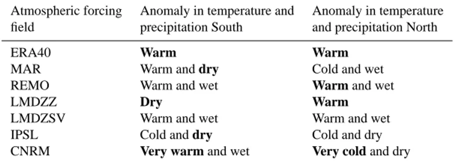
Table 3. Large scale biases of atmospheric forcing fields with respect to FE09 and key variable explaining the deviation of volume (bold).
Atmospheric forcing Anomaly in temperature and Anomaly in temperature
field precipitation South and precipitation North
ERA40 Warm Warm
MAR Warm and dry Cold and wet
REMO Warm and wet Warm and wet
LMDZZ Dry Warm
LMDZSV Warm and wet Warm and wet
IPSL Cold and dry Cold and dry
CNRM Very warm and wet Very cold and dry
considered forcing field is consequently too dry (dVi0> dVi) but also too warm (dV0> dVi0).
– dVi < dV0< dVi0: as for the previous case, the use of the Ettema et al. (2009) precipitation map increases the simulated volume, but here the final volume anomaly is greater than the reference one. The considered forcing field is consequently too dry (dVi0> dVi) and too cold
(dVi0> dV0).
– dVi0< dVi< dV0: the simulated volume is even lower with the use of the Ettema et al. (2009) precipitation
map. The considered forcing field set is consequently too wet (dVi> dVi0) and too warm (dV0> dVi0). This
case indicates a much warmer atmospheric model, be-cause even if it is wetter, the ISM simulated volume is still below the reference volume.
The second family of results corresponds to a simulated volume anomaly greater than the reference, dVi> dV0. This positive anomaly can be due to too wet conditions or/and to too cold conditions. Again three sub-cases can be identified:
(a)
(b)
(c)
(d)
Fig. 9. Regional volume difference (simulated volume minus initial volume, being 1.10 and 0.46 10
6km
3for North and South respectively) for each model run. Empty bars correspond to the standard volume
difference (dV
i) and hatched bars correspond to the volume difference computed with the precipitation
in each model replaced by the Ettema et al. (2009) precipitation map (dV
i0). The first solid bar is the
simulated reference volume difference (dV
0, FE09). The upper panel corresponds to the South region
(latitudes lower than 68
◦N) at 0.5 kyr (a) and 20 kyrs (b), and the lower panel corresponds to the North
region (latitudes greater than 75
◦N) at 0.5 kyr (c) and 20 kyrs (d).
47
Fig. 9. Regional volume difference (simulated volume minus initial volume, being 1.10 and 0.46 106km3for north and south, respectively) for each model run. Empty bars correspond to the standard volume difference (dVi) and hatched bars correspond to the volume difference
computed with the precipitation in each model replaced by the Ettema et al. (2009) precipitation map (dVi0). The first solid bar is the simulated reference volume difference (dV0, FE09). The upper panel corresponds to the south region (latitudes lower than 68◦N) at 0.5 kyr (a) and 20 kyrs (b), and the lower panel corresponds to the north region (latitudes greater than 75◦N) at 0.5 kyr (c) and 20 kyrs (d).
– dVi0> dVi> dV0: the use of the Ettema et al. (2009) precipitation map increases the simulated volume, aug-menting the positive volume anomaly. The considered forcing field is consequently too dry (dV0
i > dVi) and
too cold (dV0
i > dV0). Note that this case suggests that
the atmospheric model is strongly cold biased, because even if it is drier, the ISM simulated volume is larger than the reference volume.
– dVi > dVi0> dV0: in this case, the use of the Ettema
et al. (2009) precipitation map decreases the simulated volume, which still stays above the reference volume anomaly. The considered forcing field is consequently too wet (dVi > dVi0) and too cold (dVi0> dV0).
– dVi > dV0> dVi0: as for the previous case, the use of the Ettema et al. (2009) precipitation map decreases the simulated volume, which becomes lower than the refer-ence one. The considered forcing field is consequently too wet (dVi > dVi0) and too warm (dV0> dV
0 i).
The relative importance of temperature and precipitation on the simulated ice sheet state can be evaluated considering the amplitude of the deviation of the simulated volumes com-pared with the reference volume. When the value of dV0
i is
close to dV0, it means that precipitation is the key factor explaining simulated volume anomaly differences. Temper-ature in this case is secondary. On the other hand, when dVi0 and dVi are similar, temperature differences have to be
con-sidered as the key factor.
Following this classification and with the simulated vol-ume differences plotted in Fig. 9, we can identify the main bias of the atmospheric models in terms of glaciological re-sponse and the key variable for the north and south regions (see Table 3).
The warm models generally retreat in the north, even if they often present a relatively high precipitation anomaly. For instance, the two models presenting a collapse of the northern part, ERA40 and REMO, present a warm bias and the deviation of volume is attributable to temperature only. It
Fig. 10. Volume loss (down-pointing triangle) and gain (up-pointing triangle) as a function of July
mean temperature. The tendency lines are also plotted (we omitted the two warmest models, ERA40
and REMO, for the tendency calculation of the North volume loss on the long-term response). The lost
(resp. gained) volume is defined as the sum of the negative (resp. positive) thickness variation multiplied
by the ISM grid cell area. On the left (a), the volume deviations after a 500-yr simulation and, on the
right (b), after a 20-kyr simulation. Each pair of traingles (down and up-pointing) represent a particular
atmospheric model.
48
Fig. 10. Volume loss (down-pointing triangle) and gain (up-pointing triangle) as a function of July mean temperature. The tendency lines are
also plotted (we omitted the two warmest models, ERA40 and REMO, for the tendency calculation of the north volume loss on the long-term response). The lost (resp. gained) volume is defined as the sum of the negative (resp. positive) thickness variation multiplied by the ISM grid cell area. On the left (a), the volume deviations after a 500-yr simulation and, on the right (b), after a 20-kyr simulation. Each pair of traingles (down and up-pointing) represent a particular atmospheric model.
appears that the range of the simulated volume is mainly at-tributable to air temperature differences between the forcings in the north (3 out of 8 cases for near surface temperature, 0 out of 8 for precipitation) and precipitation differences in the south (3 out of 8 for precipitation, 1 out of 8 for near surface temperature).
Hence, the northern region appears to be highly sensi-tive to air temperature and is more prone to larger volume changes than the southern region. We, therefore, investigate in the next section whether a given warm/cold bias has the same impact on ice volume in the North and in the South.
3.4 Sensitivity of the ISM to the July temperature
Figure 10 presents the anomalies of gained and lost volume for the various regions against the mean July temperature in the corresponding region for each of the eight atmospheric forcing fields. We distinguish short-term (500 yrs) and long-term (20 kyrs) responses in volume anomaly. Each point on the temperature axis corresponds to a specific forcing field. There is a wide spread in the north region temperature among the models: the range of the simulated temperatures over the northern region is 10◦C, while it is less than 5 ◦C for
the southern region. In the south for both short-term and long-term response, the volume loss, which is close to 0 in most cases, is insensitive to an increase in temperature. The volume gain in this region, however, increases with rising temperatures in the short-term, but decreases slightly with increasing temperatures in the long-term. This means that the south region gains mass with a temperature increase, at greater rates for the short-term response than for the long-term response.
In the north, for both the short-term and long-term re-sponses, an increase in the mean July temperature results in a decrease of volume gain and increase of volume loss. In the long-term response, we can observe a threshold for the July temperature around –2◦C, above which the volume loss increases drastically. The medium region is intermediate, re-sponding more like the north in the short term and more like the south for the volume loss in the long term.
3.5 Importance of surface elevation change feedback
Sea level rise projections generally use complex climate models with fine resolution and/or sophisticated physics. ISMs are not yet included in these models and in this section we want to assess the importance of including the elevation change feedback for the ISM computation of SMB.
For this, the ISM is forced with the 8 atmospheric fields again (Table 2), but without the topographic lapse rate cor-rection. In these conditions, temperature and precipitation re-main constant during all of the simulation.
The evolution of the difference of ice volume in the ex-periment where the elevation change feedback is switched off with respect to the standard correction experiment for the south and north regions is presented in Fig. 11. The two re-gions show a completely different response.
In the south, all the runs result in a volume closer to obser-vations when we do not take into account the surface eleva-tion change feedback. Considering that the volume anomaly is systematically positive in this region (see Fig. 7a), the ex-periment without the correction of temperature and precipi-tation due to surface elevation change presents a better agree-ment with the initial state. As we already agree-mentioned, due to its resolution, the ISM is not adapted to reproducing steep
(a)
(b)
Fig. 11. Evolution of the difference between the experiment in which the surface elevation change
feed-back on temperature and precipitation is not taken into account, minus the standard correction
experi-ment. On the left (a), the South region (latitudes lower than 68
◦N) and on the right (b), the North region
(latitudes greater than 75
◦N).
49
Fig. 11. Evolution of the difference between the experiment in which the surface elevation change feedback on temperature and precipitation
is not taken into account, minus the standard correction experiment. On the left (a), the south region (latitudes lower than 68◦N) and on the right (b), the north region (latitudes greater than 75◦N).
slopes such as those observed in the south. The resulting spread leads to an increase of the elevation in the peripheral area, initially in the ablation zone, but with a high value of precipitation. With the topographic lapse rate correction, the ISM turns this warm and very high precipitation zone into a mild/cold high precipitation zone. The resulting displace-ment of the equilibrium line is, hence, a direct consequence of the downscaling method and of the resolution of the ISM. In the north, all the simulations present a bigger ice sheet when the surface elevation change feedback on temperature and precipitation is not taken into account. The only excep-tion is IPSL, i.e., the only model that retreats and has a cold and dry bias. For this model, the dry anomaly causes a gen-eral thinning of the ice sheet. A warming and a consequent increase of precipitation is observed when the surface eleva-tion change feedback is taken into account. Two model runs (REMO and ERA40) present a huge difference whether the surface elevation change feedback is taken into account or not. Those two models present a collapse of the north of the GIS (see Fig. 6a) in the standard experiment, but when the surface elevation change feedback is switched off, the ice sheet stabilises and is still present at the end of the run. The surface elevation change feedback on temperature and pre-cipitation accelerates and, thus, accentuates the retreat.
The forcing fields that show a volume increase in the North (MAR and CNRM) produce a slightly bigger volume when the feedback is switched off. This is mainly due to the al-ready cold bias in those forcings (see Sect. 3.3), resulting in an advance of ice over an area which normally is tundra zone. We can conclude that the surface elevation change feed-back on temperature and precipitation is an important driver for the forcing fields with temperature as a predominant vari-able, accentuating the biases (north case). However, when precipitation is the driver, this feedback tends to reduce the
deviation (south case). It also appears that we cannot discard this feedback for simulations lasting more than a thousand years.
4 Conclusions
In the face of uncertainties on future climate, we need to de-velop tools to predict the coupled climate-ice sheet evolu-tion for the coming centuries. The first step in this develop-ment should be to validate the uncoupled approach and to do so, we have performed here a sensitivity study of an ice sheet model (ISM) to atmospheric forcing fields. We have ap-plied several atmospheric forcing fields to an ISM in climatic steady state experiments. We have shown major discrepan-cies in the simulated ice sheets resulting from the different atmospheric forcing fields due to the tendency of the ISM to integrate the biases in the atmospheric forcings. Apart from the numerical and physical differences among the climate models, the model resolution also plays a role in explain-ing the range of model results. Usexplain-ing the same interpolation method for all forcing fields, we do not find a systematic dif-ference between regional climate models and global GCMs. Nonetheless, some of the models seem to be inappropriate for absolute forcing. For these models, we suggest the use of an anomaly method, in which the ISM is forced with the best available present day climatology plus anomalies computed by the climate model as a perturbation, instead.
Although July temperature seems to be important for the ISM behaviour, in particular in the northern part of the GIS, precipitation may also play an important role, particularly in the south. We have shown that the north of Greenland is more sensitive to temperature anomalies than the south and we sus-pect that major changes are likely to occur there in a warmer climate. The south seems to be relatively stable and almost
over several thousand years, even though it is of secondary order compared with atmospheric model biases. While the most common way to downscale surface temperature forcing fields from climate model to ISM is using a relatively uncon-strained topographic lapse rate, specific experiments have to be performed.
The current ISM is unable to accurately reproduce the southern ice sheet topography because it does not take into account the very fine scale processes taking place in this re-gion. To improve on this, in addition to a finer ISM grid, very fine resolution atmospheric forcing fields and better down-scaling techniques are required, such as those proposed by Gall´ee et al. (2011).
Supplementary material related to this article is
available online at: http://www.the-cryosphere.net/6/999/ 2012/tc-6-999-2012-supplement.pdf.
Acknowledgements. We thank CISM for providing the datasets
of Shapiro and Ritzwoller (2004); Joughin et al. (2010); Burgess et al. (2010); van der Veen et al. (2001). Janneke Ettema, Jan van Angelen and Michiel van den Broeke (IMAU, Utrecht University) are thanked for providing RACMO2 climate fields. We thank Konrad Steffen and the DMI for providing temperature data for the Greenland weather stations. Aur´elien Quiquet is supported by the ANR project NEEM-France. NEEM is directed and organized by the Center of Ice and Climate at the Niels Bohr Institute and US NSF, Office of Polar Programmes. It is supported by funding agencies and institutions in Belgium (FNRS-CFB and FWO), Canada (NRCan/GSC), China (CAS), Denmark (FIST), France (IPEV, CNRS/INSU, CEA and ANR), Germany (AWI), Iceland (RannIs), Japan (NIPR), Korea (KOPRI), The Netherlands (NWO/ALW), Sweden (VR), Switzerland (SNF), UK (NERC) and the USA (US NSF, Office of Polar Programs). Heinz-J¨urgen Punge is supported by the European Commission FP7 project 226520 COMBINE and the ANR project NEEM-France. This work was supported by funding from the ice2sea programme from the Eu-ropean Union 7th Framework Programme, grant number 226375. Ice2sea contribution number ice2sea066. All (or most of) the computations presented in this paper were performed using the
The publication of this article is financed by CNRS-INSU.
References
´
Alvarez-Solas, J., Charbit, S., Ramstein, G., Paillard, D., Du-mas, C., Ritz, C., and Roche, D. M.: Millennial-scale os-cillations in the Southern Ocean in response to atmo-spheric CO2 increase, Global Planet. Change, 76, 128–136, doi:10.1016/j.gloplacha.2010.12.004, 2011.
´
Alvarez-Solas, J., Montoya, M., Ritz, C., Ramstein, G., Charbit, S., Dumas, C., Nisancioglu, K., Dokken, T., and Ganopolski, A.: Heinrich event 1: an example of dynamical ice-sheet reaction to oceanic changes, Clim. Past, 7, 1297–1306, doi:10.5194/cp-7-1297-2011, 2011.
Amante, C. and Eakins, B.: ETOPO1 1 Arc-Minute Global Relief Model: Procedures, Data Sources and Analysis, NOAA Techni-cal Memorandum NESDIS NGDC-24, p. 19, 2009.
Arthern, R. J. and Gudmundsson, G. H.: Initialization of ice-sheet forecasts viewed as an inverse Robin problem, J. Glaciol., 56, 527—533, doi:10.3189/002214310792447699, 2010.
Bamber, J. L., Layberry, R. L., and Gogineni, S. P.: A new ice thick-ness and bed data set for the Greenland ice sheet 1. Measurement, data reduction, and errors, J. Geophys. Res., 106, 33773–33780, doi:10.1029/2001JD900054, 2001.
Bintanja, R., van de Wal, R. S. W. and Oerlemans, J.: Global ice volume variations through the last glacial cycle simulated by a 3-D ice-dynamical model, Quatern. Int., 95–96, 11–23, doi:10.1016/S1040-6182(02)00023-X, 2002.
Born, A. and Nisancioglu, K. H.: Melting of Northern Greenland during the last interglacial, The Cryosphere Discuss., 5, 3517– 3539, doi:10.5194/tcd-5-3517-2011, 2011.
Brun, E., David, P., Sudul, M., and Brunot, G.: A numerical model to simulate snow-cover stratigraphy for opera tional avalanche forecasting, J. Glaciol., 38, 13–22, 1992.
Bueler, E. and Brown, J.: Shallow shelf approximation as a “sliding law” in a thermomechanically coupled ice sheet model, J. Geo-phys. Res., 114, F03008, doi:10.1029/2008JF001179, 2009. Burgess, E. W., Forster, R. R., Box, J. E., Mosley-Thompson, E.,
Bromwich, D. H., Bales, R. C., and Smith, L. C.: A spatially calibrated model of annual accumulation rate on the Greenland Ice Sheet (1958–2007), J. Geophys. Res.-Earth, 115, F02004, doi:10.1029/2009JF001293, 2010.