Any correspondence concerning this service should be sent to the repository administrator:
[email protected]
Identification number:
DOI : 10.1016/j.jfluidstructs.2013.11.005
Official URL:
http://dx.doi.org/10.1016/j.jfluidstructs.2013.11.005
This is an author-deposited version published in:
http://oatao.univ-toulouse.fr/
Eprints ID: 11252
To cite this version
:
Harran, Gilles Influence of the Mass ratio on the fluid-elastic instability of a
flexible cylinder in a bundle of rigid tubes.
(2014) Journal of Fluids and
Structures, vol. 47 . pp. 71-85. ISSN 0889-9746
Open Archive Toulouse Archive Ouverte (OATAO)
OATAO is an open access repository that collects the work of Toulouse researchers and
makes it freely available over the web where possible.
Influence of the mass ratio on the fluidelastic instability
of a flexible cylinder in a bundle of rigid tubes
G. Harran
nInstitut de Mécanique des Fluides de Toulouse, 6 allée du Prof. C. Soula, 31400 Toulouse, France
Keywords: Fluidelastic instability Tube bundles Cross-flow Root locus a b s t r a c t
Several linear lumped-parameter models were proposed in the past to identify the main mechanisms underlying the cross-flow instability of a single flexible cylinder in tube bundles. Basing on such models, we analyze the influence of the mass ratio when the cylinder vibrates in the transverse direction, without structural damping (corresponding to a zero Scruton number). For two selected mass ratios, we focus on this linear interaction plotting the poles of the fluid–structure system as a function of the reduced velocity (root locus). This asymptotic approach allows a better understanding of the combined influence of the transient fluidelastic coupling and the mass ratio.
1. Introduction
The fluidelastic interaction in cylinder arrays is complex, since it combines three types of instability (Khalifa et al., 2012;
Païdoussis et al., 2010;Blevins, 1994):
Instability by antisymmetric stiffness similar to classical flutter, with at least two degrees of freedom involved in the motion. It is the main mechanism when reduced velocity is much higher than unity.
Dynamic instability for a Single-Degree-Of-Freedom cylinder. It is the main mechanism when reduced velocity is of the order of unity.
Static instability (divergence) for a Single-Degree-Of-Freedom cylinder. It was highlighted byPaidoussis et al. (1989)for
peculiar geometrical patterns.
The difficulty to differentiate these instabilities can be evoked as one of the reason for the high experimental scattering on the values of critical velocity Ucor the reduced critical velocity
Urc¼
Uc
fSD;
where fSis the structural natural frequency and D the cylinder diameter. In addition to the geometric pattern influence,
Ucis affected by other phenomena:
Vortex-Induced-Vibration domain and Movement-Induced-Vibration domain overlap when Scruton number is low (Weaver, 2008). According toGranger and Paidoussis (1996), this can explain some modeling difficulties for fluidelastic instability prediction.
http://dx.doi.org/10.1016/j.jfluidstructs.2013.11.005
n
Tel.: þ33 534 32 28 84.
The Reynolds number strongly influences the physics of the flow, but it is very seldom taken into account.Gillen and Meskell (2008)show an important influence on the static efforts and notable consequences on the critical velocity by the
quasi-unsteady model ofGranger and Paidoussis (1996).
This critical velocity value is a crucial criterion for design of heat exchangers. It is usually plotted as a function of the mass
ratio (m⋆) and reduced structural damping (ξ
S), defined inTable 1. The three constants K, p, q in relation(1)
Urc¼ Kðm⋆ÞpξqS ð1Þ
are then fitted from experimental data. The Scruton number (Sc ¼ 2πξSm⋆
) appears if p¼q is considered. This dimensionless
group quantifies the ratio between the energy dissipated by the structure and the energy taken from the fluid (Axisa, 2001).
Since experimental evidence of a specific dependence to the structural damping and the mass ratio are numerous (Tanaka and
Takahara, 1981;Price, 2001), it is not relevant to assume that p¼q, as suggested by Connors-type equations (Connors, 1970). Some efforts are still necessary to unfold the specific influence of the mass ratio and reduced structural damping
according to the value range of the Scruton number (Weaver, 2008). In order to contribute to this analysis, we propose to
isolate the influence of the mass ratio, considering an undamped structure, which corresponds to the asymptotic case Sc-0. The linear models with lumped-parameter approach will be considered, leading to a user-friendly description of the fluidelastic instability in cross-flow cylinder arrays. Nevertheless, they show substantial weakness in accurately predicting
critical velocities for specific industrial applications such as steam generators (Price, 2001). This industrial application is
characterized by low Scruton numbers and reduced velocities of the order of unity. That implies a strong fluidelastic
coupling and the need for taking into account of the transients of the coupling mechanism (Tanaka and Takahara, 1981).
For a bibliographical synthesis on these phenomena and the various modeling options to predict these instabilities (generally referred as damping-controlled instability), one can consult (Price, 2001;Païdoussis et al., 2010).
We propose to distinguish two classes of models, according to whether the fluid–structure system is described by:
a model of the same order as that of the structure model order. The interaction is then characterized by a damping coefficient and a stiffness coefficient added by the flow, which depend on the reduced velocity, since the quasi-static
theory is not valid. It is for example the approach ofChen (1987).
a model of a higher order than that of the structure model order. The interaction is identified by its own dynamics. It is for
example the approach ofPrice and Païdoussis (1986)orGranger and Paidoussis (1996), that we will compare (Section 2.3).
The model ofLever and Weaver (1982)also belongs to this category.
In order to analyze the influence of the mass ratio on the loss of stability, it is necessary to precisely describe the dynamics of the interaction and not only its consequences on the dominant mode of the coupled system. Only the second category of models can thus bring elements of physical insight. This is why we will limit the discussion to this class of models. Only linear models are considered here, but the nonlinear tools for simulation are set up for the continuation of the study. We will use the symbolic formalism for its ease of handling, although the temporal formulation by the operator of convolution is more explicit in describing the physics of the memory.
All the cylinders are fixed, except the central one that is flexibly mounted. It can move in the z direction only in an in-line
square array, with P the pitch between cylinders (Fig. 1). The ratio between the pitch velocity Upand the free-stream single
Table 1
Nominal parameters for the experiment and simulations.
Parameter Notation Value
Fluid density (kg m% 3) ρ F 1.2 Dynamic viscosity (m2s% 1) ν 15 & 10% 6 Cylinder length (m) L 0.6 Cylinder diameter (m) D 0.08 Pitch (m) P 0.12 Pitch ratio P=D 1.5 Aspect ratio a ¼ ðP=DÞ=ðP=D%1Þ 3 Total mass (kg) MS 0.5
Mass per length (kg/m) m ¼ MS=L 0.83
Structural damping coefficient (N/(ms% 1)) C
S 0
Structural stiffness coefficient (N m% 1) K
S 3000
Structural reduced damping ξS 0
Structural natural frequency (Hz) fS 12.3
Structural natural frequency (rd/s) ωS 77.46
Pitch Reynolds number Re ¼ UpD=ν 51 500
Mass ratio m⋆
¼ m=ðρFD2Þ 108
Scruton number Sc ¼ 2πξSm⋆ 0
phase flow velocity U is the aspect ratio a ¼ Up=U ¼ ðP=DÞ=ðP=D%1Þ. The numerical values of the simulated configuration and
the notations are given in Table 1. It corresponds to an experimental setup under development in a wind tunnel, with
virtualization of the dynamics of structure as proposed by Hover et al. (1998) and later by Mackowski and Williamson
(2011). This concept will allow the experimental study of the asymptotic case of an undamped structure (ξS¼ 0), analyzed in this paper.
2. Fluidelastic models
After a short presentation of the interaction concept with a block diagram representation (Preumont, 2002), the
fluidelastic coupling models based on the lumped-parameter approach are recalled and discussed.
2.1. Block-diagram representation
Following a common assumption (Chen and Jendrzejczyk, 1983), the fluid loading on the structure F can be separated
into two terms: a force non-correlated to the cylinder movement FzðtÞ and a force correlated to the cylinder movement
FzðtÞ, leading to
FðtÞ ¼ FzðtÞþFzðtÞ: ð2Þ
The feedback nature of fluidelastic systems is considered by a functional diagram representation (Fig. 2). This concept allows
to characterize the stability of the closed-loop system with the control theory, as emphasized byFung (1955).
The fluidelastic operator models the feedback of the structure movement on the fluid loading. The structural operator represents the dynamics of the structure. There are differences in the behavior of the structure in vacuum and in quiescent fluid. These differences are important when the mass ratio is low and they are generally taken into account by an added mass and possibly an added damping. In this paper, the term structure refers to the structural behavior in quiescent fluid. So, added mass and added damping are included into the structure parameters.
As a first step, it is often considered that the excitation term of the feedback system FzðtÞ represents turbulence-induced
forces (random and deterministic). But on the one hand, the wake-oscillator concept can be used alternatively to model
organized eddies (de Langre, 2006) by a coupling with the structure-oscillator. Lock-in is then interpreted as a
classical-flutter instability. This linear model gives a description of the interaction between the structure movement and organized-eddies. On the other hand, the organized eddies impact the random turbulence properties: the Von Kármán vortices cause an imbalance between production an dissipation of the turbulent energy cascade, which changes the slope of the power
spectral density in the inertial domain, as demonstrated by Braza et al. (2006). So, which part of turbulence has to be
interpreted as the excitation loading for the closed-loop system? Aware of the difficulty to clearly define the frontier of the system, we will analyze the stability problem for the Movement-Induced-Vibrations without
Turbulence-Induced-Vibrations or Vortex-Induced-Turbulence-Induced-Vibrations with the functional diagram of Fig. 2. We choose a Linear Time Invariant
Fig. 1. Flexibly mounted cylinder in an in-line square array.
representation for both structural and fluidelastic operators. This assumption restricts the model validity around an
equilibrium point considering small variations for the state of the system. The equation of the dynamics represented inFig. 2
can be expressed as
MS€z þCS_z þKSz ¼ FzðtÞþFzðtÞ: ð3Þ
In the Laplace domain this leads to the structural transfer function connecting the position variations and the global fluid loading F ðtÞ
zðpÞ
FðpÞ¼
1
KSþCSp þMSp2;
which is coupled with the fluidelastic transfer function %FzðpÞ=zðpÞ, leading to the closed-loop transfer function zðpÞ=FzðpÞ. Notations are the same in both temporal and Laplace domains and p ¼ xþjy is the symbolic variable.
2.2. Fluidelastic transfer function
Generally, the lumped-parameter models for fluidelastic coupling define static parameters and dynamical parameters.
Lever and Weaver (1986)describe flow structure (the wake region and the channel region) with static parameters and determine the global load by integrating the pressure over the attached region. The static part of coupling can also result
from the drag coefficient CD and the lift coefficient CLas functions of the cylinder position z, on which they necessarily
depend because of the presence of the adjacent tubes (Price and Païdoussis, 1986;Granger and Paidoussis, 1996). By taking
the convention of positive displacement downwards (Fig. 1), Eq. (4) is the expression of the force correlated with the
movement
Fzð Þ ¼ %T sin α%P cos α ¼ %t 12ρFU2relDL C½ Dðz; _zÞ sin αþCLðz; _zÞ cos α(: ð4Þ
The linearization of the force coefficients (Price and Païdoussis, 1986) leads to
CD¼ CD0þ ∂CD ∂z 0z ¼ CD0; and CL¼ CL0þ ∂CL ∂z 0z ¼ ∂CL ∂z 0z;
since at the equilibrium point CL0¼ ∂CD=∂zj0¼ 0, for symmetry reason. The subscript 0 corresponds to static values
for the equilibrium point.
With the linear assumptions (seeFig. 1) α ¼ _z=U and Urel¼pffiffiffiffiffi_z2þU2* U, the force model can be written as Fzðz; _z; tÞ ¼ %1 2ρFU2DL CD0 _z U þ ∂CL ∂z 0z # ¼ %Ca0_z %Ka0z; $ ð5Þ with Ca0¼ 1 2ρFUDLCD0; Ka0¼ 1 2ρFU 2L∂CL ∂z⋆ 0; z⋆ ¼Dz:
This formulation(5)reflects two effects
An added damping (Ca0) function of the drag. This is the stabilizing effect of the drag (as in galloping instability),
An added stiffness (Ka0) function of the lift variations with the cylinder position. Measurements show that Ka040, in the
vast majority of tube bundle patterns.
For most geometric patterns, a dynamic instability occurs when reduced velocity is of the order of unity, whereas the
quasi-static model(5)predicts unconditional stability. This model must be modified to take into account of the transient
effects. In the quasi-unsteady model,Granger and Paidoussis (1996)propose to convolve z(t) the tube displacement into
Eq.(5)with h(t) the impulse response of a linear filter. Eq.(6)models the transient process of the lift generating.
Fzðz; _z; tÞ ¼ %1 2ρFU 2DL C D0 _z U þ ∂CL ∂z 0z⋆h tð Þ # : $ ð6Þ In the Laplace domain, the impulse response of the filter h(t) becomes the transfer function HðpÞ ¼ L½hðtÞ( for zero initial conditions, as illustrated inFig. 3.
If the need for introducing a phase delay to explain instabilities of tube bundles is relatively recent, the aerodynamic community has considered the importance of transients in flutter models approximately sixty years before, with the works ofWagner (1925). Nowadays, modeling is extended to the nonlinear analysis considering the Volterra series or High Order Spectral Analysis (Silva, 2005).
A distinction can be drawn between coupling models depending on whether the process is assumed with memory effects or memoryless:
memoryless. This is the time delay model (Price and Païdoussis, 1986;Lever and Weaver, 1986) characterized by
HðpÞ ¼ e% Tp;
or
hðtÞ ¼ δðt %TÞ:
The phase lag ϕðωÞ ¼ %ωT is unbounded since it is proportional to the frequency.Price and Païdoussis (1986)propose
β¼ 1=a for the time-constant T ¼ βD=U.
with memory. The transfer function H(p) is then a rational fraction and the phase lag is bounded.Granger and Paidoussis (1996)propose a first-order model and a two-order model. The first-order model is defined by the step response of the filter
ΘðtÞ ¼ ð1%α1e% δ1aU=DtÞuðtÞ;
with u(t) the Heaviside function. It illustrates the memory of the initial condition and is also referred as the Wagner function. The transfer function is
H pð Þ ¼ L dΘðtÞ dt
$ #
¼ pL Θ t½ ð Þ( ¼ 1% α1p
pþδ1aU=D:
By defining the two time-constants T2¼ β2D=U and T1¼ β1D=U where β1¼ 1=δ1a and β2¼ β1ð1%α1Þ, the transfer
function can be expressed on the following form:
H pð Þ ¼1þT2p
1þT1p: ð7Þ
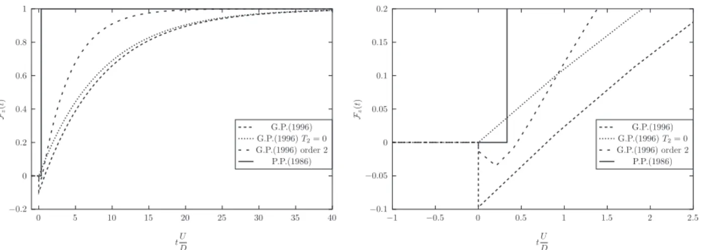
Fig. 4 shows this memory function for an in-line square array with a pitch ratio P=D ¼ 1:5. The constants α1; δ1 were
obtained empirically byGranger and Paidoussis (1996) to fit with the critical velocity obtained by experiments.Meskell
(2005)proposes a direct determination of the constants by modeling of the non-stationary wake by vortex method. The step
response for the model of Price and Païdoussis (1986)is also displayed (Fig. 4) with the one obtained by the first-order
model of Granger and Paidoussis (1996)without numerator (T2¼ 0), as suggested byMeskell (2005). This model will be
used thereafter for two reasons:
The second order model does not induce great modification to the memory function for an in-line square array and gives critical velocities very close to those obtained by a first-order model.
As α141 (Granger and Paidoussis, 1996), then T2o0 in Eq.(7)and the step response presents a paradoxical behavior at the origin, since the force is negative before the change of sign. This phenomenon was not identified by the authors since
it does not appear on the step response schematized in reference (Granger and Paidoussis, 1996). It is not very marked for
an in-line square array because T2{T1, in contrast with a rotated pattern (Meskell, 2005). Without any other justification to accredit this paradoxical form, it will not be adopted here. A specific study of sensitivity to the zero of H(p) is proposed below (cf.Section 4).
The first-order model of filtering chosen here is defined by its impulse response (with T ¼ T1)
h tð Þ ¼1 Te% t=T;
or its transfer function
H pð Þ ¼ 1
1þTp: ð8Þ
Classically, the time constant of the first-order model is a function of the time-scale of advection TA¼ D=U with β such that
T ¼ βDU:
It is the form which gives the quasi-static model asymptotically (HðpÞ ¼ 1) when Tp-0, or in frequential terms when βDω=U-0, or Ur-1 considering ω ¼ ωSto obtain a global definition of the quasi-static assumption. An attempt to improve
this time-constant model is proposed byHémon (1999). The diffusion time-scale is certainly at least as important as because
it is implied in the physique of separation. This remark justifies the need for considering the Reynolds number effects. This low-pass first-order model has three parameters CD0, ∂CL=∂zj0, β, that is to say the same parameters as for the
time-delay model. The models with or without memory effects can thus be of the same level of complexity. The first two parameters are static parameters and are derived from the drag and lift coefficients at the equilibrium point. They depend
on the pattern of the cylinder array and on the Reynolds number (Mahon and Meskell, 2012). The model ofLever and
Weaver (1982)also includes static parameters but in greater number to describe the geometry of the stream tube. The third parameter is the dynamic one which fixes the time-constant of the mechanism of coupling. For the in-line square array with
P=D ¼ 1:5, the parameter values were obtained from the literature as forGranger and Paidoussis (1996)and are given in
Table 2. After analyzing the analogy of both models, we can compare them for two asymptotic situations.
2.3. Phase-lag models for asymptotic values of Sc
To compare the ability of the phase-lag models (bounded or unbounded) to estimate the critical velocity of instability, two asymptotic cases with respect to the Scruton number are considered. The stability criterion for high Scruton numbers of
Price and Païdoussis (1986)is demonstrated by a different way and a new stability criterion for low Scruton numbers is proposed.
2.3.1. Stability criterion for high Scruton numbers
For high Scruton numbers, the reduced critical velocity is large. It can therefore be estimated considering Tpo1 in the transfer function H(p). So we have
1
1þTp* 1%Tp;
Fig. 4. Memory function for an in-line square array P=D ¼ 1:5. Table 2
Parameters of the coupling model.
Parameter Notation Value
Drag coefficient (Price and Païdoussis, 1986) CD0 2.3 Lift coefficient gradient (Price and Païdoussis, 1986) ∂CL
∂z⋆j0
73 Denominator reduced time-constant
(Granger and Paidoussis, 1996)
β1 8.55
Numerator reduced time-constant (Granger and Paidoussis, 1996)
as it is the case for a memoryless model (Price and Païdoussis, 1986) e% Tp* 1%Tp:
Thus the approximation is the same for both models, whether it is for a time-delay model or a first-order low-pass filter
model. The same approximation is valid for model in Eq.(7)since T2oT1 and
1þT2p
1þT1p *1% Tð 1%T2Þp:
The functional diagram inFig. 5shows this asymptotic model for high Scruton number.
The stability condition is expressed by the relation CSþCG40 with
CG¼ CD0%β
∂CL ∂z⋆ 0:
Formally, the expression(9)obtained byPrice and Païdoussis (1986)is the same to the galloping instability criterion
Urc¼ 4
jCGjSc: ð9Þ
However, since this result is valid only for high Scruton numbers, this tube-array instability should not be confused with the galloping instability.
The time-delay model and the low-pass first-order model are equivalent to determine the critical velocity for high
Scruton numbers. They show that the reduced critical velocity is proportional to the Scruton number. The paper ofGranger
and Paidoussis (1996) is in agreement with this result for a rotated pattern but not for an in-line square pattern with
UrcppffiffiffiffiffiSc, which is not coherent with relation(9). It is however the behavior retained byPrice (2001)orPaïdoussis et al.
(2010)in their synthesis book.
2.3.2. Stability criterion for low Scruton numbers
For low Scruton numbers, the reduced critical velocity is of the order of unity, but taking into account β value, the critical velocity can be estimated with the approximation
1
1þTp*
1
Tp; ð10Þ
that is sketched in the functional diagram ofFig. 6.
The analysis of stability by the Nyquist criterion (Fung, 1955;Preumont, 2002) shows that the threshold of stability is reached when the magnitude of the open-loop Frequency-Response-Function equals one and phase-lag takes the value 1801. This is for the natural frequency of the structure ωS. That leads to
Uc¼
CSþCa0
Ka0MS
βDKS: ð11Þ
Fig. 5. Asymptotic model for high Scruton numbers.
If the structural damping (CS) is negligible compared to the damping induced by the drag (Ca0) or if like here CS¼0, the critical velocity is Uc¼ ffiffiffiffiffiffiffiffiffiffiffiffiffiffiffiffiffiffiffiffi CD0βD ∂CL ∂z 0ωn: v u u u t
The reduced critical velocity is
Urc¼ 2π ffiffiffiffiffiffiffiffiffiffiffiffiffiffi CD0β ∂CL ∂z⋆ 0; v u u u t ð12Þ
or if the pitch velocity is used as reference
Uprc¼ 2πa ffiffiffiffiffiffiffiffiffiffiffiffiffiffi CD0β ∂CL ∂z⋆ 0: v u u u t
The critical velocity is asymptotically bounded when Sc-0. It justifies the very weak influence of structural damping
observed in practice on the critical velocity for low Scruton numbers (Price, 2001). This behavior is in perfect agreement
with the formulation of the model, despite it is often regarded as paradoxical (Weaver, 2008). Confusion arises that it is not
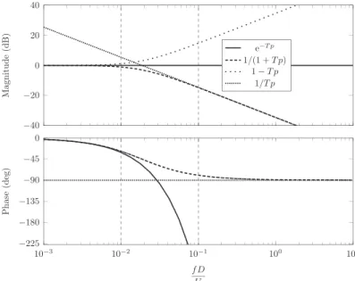
exactly, as generally reported, an instability controlled by damping but by the transient of the fluidelastic coupling. To identify the validity domains for both asymptotic models, the Bode plot for all the one-time-constant models is given inFig. 7. The cut-off reduced frequency (%3 dB, %45) for the first order model is f% 3 dB
r ¼ 1=2πβ ¼ 0:0186. If it is considered
that the structure frequency is representative of the dominant oscillatory mode to define a global criterion, the validity of the asymptotic models is roughly conditioned by the two limits:
Ur4100, then 1
1þTp* e% Tp* 1%Tp:
In this domain, the time delay model and the low-pass first-order model are identical.
Uro10, then 1
1þTp*
1
Tp:
In this domain, the time-delay model leads to very different results from the two other models, with switching stability/ instability when reduced velocity increases. The number of switches tends to infinity when the Scruton number tends to
zero. Arbitrarily,Lever and Weaver (1986)recommend to consider only three stable domains.
3. Influence of the mass ratio
To study the influence of the mass ratio, the lumped-parameter model is simulated with the software LMS Imagine.Lab
AMEsim. Later, it will also allow:
to refine the validity domain of the linear asymptotic models and to check their validity domains basing on frequency responses.
to extend the analysis to higher-order models or nonlinear models,
to develop a virtual prototype for the design of an experimental test bench.
Only the asymptotic case Sc-0 will be simulated here as it is known that, for high Scruton numbers, instability occurs because of antisymmetric stiffness and therefore the considered models are not suitable for. As the influence of the reduced
velocity Uron the closed-loop modes will be analyzed by the root locus (i.e. the evolution of the poles in the complex plane),
so we recall inFig. 8the characteristics of an oscillatory mode and of an aperiodic mode. ωnis the natural frequency, ωpthe
proper frequency and ξ the reduced damping of the oscillatory mode. T is the time constant of the aperiodic mode. A mode
is faster when the pole goes to the left in the stable part of the complex plane. It is also pointed out (Preumont, 2002) that
the m open-loop poles are the starting points of the locii for Ur-0 and the n zeros of the open-loop are the ending points
for Ur-1. When m4n the root locii follow asymptotic directions in the complex plane.
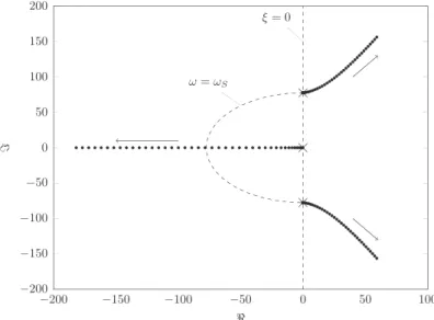
InFig. 9, the closed-loop poles are plotted for 0oUro40 with a pitch of one. The open-loop poles (Ur¼0) are marked by
crosses. The dashed lines corresponds to the stability threshold (ξ ¼ 0) and to the iso%ωScircle. The directions of the three
locii when the reduced velocity increases are indicated by arrows. The aperiodic mode coming from the origin tends rapidly towards %1. The oscillatory mode coming from the mode of structure, becomes unstable with an asymptotic direction
Fig. 8. Modal characteristics in the complex plane. (a) Oscillatory mode and (b) aperiodic mode.
Fig. 9. Root locus with varying of reduced velocity (ξS¼ 0, m⋆
when Ur-1. The critical reduced velocity Urc¼ 3:26 is exactly the value deduced from the asymptotic model of Eq.(12).
Fig. 10presents a zoom ofFig. 9tracing the root locus for 0oUro4 with a pitch of 0.2. This allows us to analyze the loss of stability of the oscillatory mode depending whether the stabilizing effect of the drag is taken into account or not. When the
reduced velocity increases, taking into account the drag (CD0¼ 2:3), the oscillatory mode begins to damp, otherwise
(CD0¼ 0) the root locus directly goes to the unstable region. The drag damping plays a dominant role for low reduced
velocity. It strongly influences the critical reduced velocity.
In order to analyze the influence of the mass ratio, the density of the fluid is increased up to ρ ¼ 1000 kg=m3. For the
same structure, the mass ratio is m⋆
¼ 0:13 (water channel experiment) instead of m⋆
¼ 108 as before (wind tunnel experiment). It is pointed out that no modification of fluid viscosity is taken into account in the model. From the root locus
for 0oUro4 (Fig. 11) we can see that the damping of the oscillatory mode increases considerably and then decreases
continuously. The maximum of the reduced damping (ξ ¼ 0:86) is obtained for a reduced velocity Ur¼1.17. The reduction in
the natural frequency of the oscillatory mode is also much more important than in air. The inversion of trend of the frequency in the vicinity of the critical velocity results in a loop in the complex plane. We will see that this loop disappears if
one takes the model of Granger and Paidoussis (1996). The critical reduced velocity Urc¼ 3:85 is slightly higher than
Urc¼ 3:26, the value predicted by the asymptotic model(12). The global comparison is good considering the root locus for
both models inFigs. 11 and 12. It appears that (i) Urcis not very sensitive to the mass ratio when ξS¼ 0 and (ii) the integrator transfer function(10), is validated for low reduced velocities.
By neglecting the stabilizing effect of the drag (CD0¼ 0) the root locus (Fig. 13) exhibits a different topology for 0oUro4.
The influence of the drag is very important, especially when m⋆is low. It is a result which can explain important differences
between the in-line and rotated patterns because the geometry of the tube arrays is of great importance for the drag value.
Fig. 10. Influence of the drag on the oscillatory mode (ξS¼ 0, m⋆¼ 108).
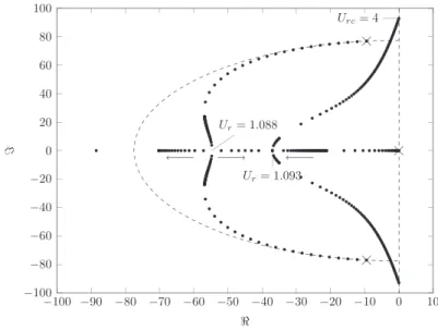
With a structural damping such as Sc ¼ 0:1, the root locus inFig. 14illustrates a behavior even more singular. To improve the representation, the step for the reduced velocity is not constant and the evolution of the fastest mode is not represented
for Ur41:1. Because of a junction of the poles of the oscillatory mode on the real axis, the system is characterized by three
aperiodic modes for 1:088oUro1:093. Beyond this value, the system has an aperiodic mode all the faster as Urincreases
and an oscillatory mode whose damping decreases and becomes zero for Urc¼ 4. In agreement with relation (11), this
critical value is slightly higher than the value Urc¼ 3:85 obtained for ξS¼ 0. 4. Sensitivity to the zero of the transfer function
In this section, we analyze the sensitivity of the first-order model to the magnitude and to the sign of the numerator time-constant T2. We compare the results obtained with the transfer function(7)in the three cases T2¼ 0, T240 and T2o0.
The last case is the choice of Granger and Paidoussis (1996). Although β2oβ1 the zero of the transfer function plays a
crucial role.
Considering T2¼ 0, for a high mass ratio (m⋆¼ 108), we showed that the natural frequency of the oscillatory mode
increases continuously with the reduced velocity (Fig. 10), especially near the stability threshold. The increase is larger for
T240 as can be seen inFig. 15. On the contrary, for T2o0 there is a reduction in the frequency of the oscillatory mode
during the crossing of the stability threshold. For higher reduced velocities (Fig. 16), the slope of the asymptote when Ur-1
is sensitive to the numerator of the transfer function H(p). For a low mass ratio (Fig. 17), this sensitivity is much more
important. If the zero is positive (T2o0) the critical velocity is much lower Urc¼ 1:15 instead of Urc¼ 3:85 if T2¼ 0. If the
zero is negative (T240) the asymptotic directions (Ur-1) is in the left half-plane; the closed-loop system is
Fig. 12. Root locus with model(10)(ξS¼ 0, m⋆¼ 0:13).
Fig. 14. Root locus (m⋆
¼ 0:13, Sc ¼ 0:1).
Fig. 15. Influence of T2on the oscillatory mode (0oUro4, ξS¼ 0, m⋆¼ 108).
Fig. 16. Influence of T2on the oscillatory mode (0o Uro40, ξ
unconditionally stable. This influence on the form of the root locus is explained by the attraction effect of the open-loop zero
since it is the ending-points of the root locus. When Ur-1, the open-loop zero tends to %1 for T240 or it tends to þ1
for T2o0. This attraction effect is used in control theory to inhibit an oscillatory mode with compensator zeros near system
poles with notch-filter technique (Preumont, 2002).
It is thus noted that the paradoxical behavior of the step response of the filter, consequence of the negative sign of T2,
may be necessary to produce a dynamic instability. In contrast to the high-mass-ratio situation, the critical velocity is now
very sensitive to the value of β2. These results show a specificity of the tube bundle configuration, since the models
classically used for airfoils and bluff bodies have always the same sign for pole and zero (Turbelin and Gibert, 2002).
The paradoxical effect in the memory function, corroborated by the experimental results ofCaillaud (1999), would thus have
a legitimacy to model the dynamics of fluidelastic coupling in tube bundles.
5. Discussion
The analysis of fluidelastic instability in tube bundles of the results is often limited to the determination of a stiffness coefficient and a damping coefficient, to model the influence of the flow on the oscillatory mode of the structure. Considering a low-pass first-order transfer function to model the forces correlated with the movement, one can simply determine the expression of these coefficients as function of the time-constant (T) of the model. For an harmonic movement of the structure zðtÞ ¼ z0sin ðωtÞ, the response of the fluidelastic model after the transient dies out is
Fzð Þjt-1t ¼ %Ka0z0 1 1þω2T2z tð Þ% ωT 1þω2T2_z tð Þ $ # :
The term in phase with the displacement is the added stiffness and the term in phase with the velocity is the added
damping.Preumont (1994)names it hereditary damping because it is the consequence of the history of the process. Both
added coefficients depend on ωD=U. The parameters of added-stiffness and added-damping are not constants but should be
considered as functions of the reduced velocity, assuming ω * ωS. In this class of models, one is not thus interested that in
the branch of the root locus which crosses the imaginary axis (cf. for exampleFig. 9), because only one oscillatory mode is
taken into account. This modeling is valid only in the vicinity of the critical velocity where the oscillatory mode dominates. The mechanism of interaction is only considered through its consequences on one of the modes and the origin of instability is not described. In addition, it is assumed that the unstable mode comes necessarily from the branch of the root locus starting from the oscillatory mode of the structure. A single-time-constant model, derived from the first-order model by
Granger and Paidoussis (1996), showed that it is not systematic when the mass number m⋆is low. The elementary model
does not take into account all the effects of the mass ratio: we omitted inertial effects in the quiescent fluid, which are
generally taken into account by an added mass, in spite of the conceptual limitations of this approach exposed bySarpkaya
(2010). It does not bring into question the first conclusion:
For physical understanding, the fluidelastic model should not be restricted to the form of a memoryless process (without an own dynamic) since the instability is controlled by memory effects. The link of the added stiffness and added damping parameters with reduced velocity is only a trivial mean to take into account this memory. It is a better way to characterize the influence of the reduced velocity on the dynamics of the closed-loop system.
Fig. 17. Influence of T2on the oscillatory mode (0oUro4, ξ
S¼ 0, m⋆¼ 0:13). –
A second element of discussion relates to the terminology often used to describe this kind of instability which may be misleading:
The term single degree of freedom instability is misleading. If the structure in the quiescent fluid is an Single Degree Of Freedom oscillator, coupling with the flow introduces other dynamics which require increasing the model order. We considered here a closed-loop system with two degrees of freedom (the modal forms will be described by two variables of observation).
The term damping-controlled suggests that a simple model of added-damping would be enough to describe the phenomenon correctly. If the reduced velocity is of the order of unity, the transients of the coupling process become important. In agreement with the experimental evidence, we showed that the critical velocity is then bounded when Sc-0. It thus becomes practically insensitive to the structural damping. We also justified that the mass ratio is an important parameter, independently of reduced structural damping, since it dramatically modifies the topology of the root locus with significant added-stiffness effects.
To avoid confusion between instability in steam generators (low Scruton numbers) and the fully damping-controlled instabilities (galloping instability), the use of a specific terminology is essential. To name fluidelastic instabilities in two phase flow where the Scruton number is low (like in steam generators), one can suggest transient-controlled instability or instability by delayed stiffness.
In this study we compared the memoryless model of time delay with a memory model considering a time-constant only.
Both models have the same level of complexity since both require only three parameters: CD, ∂CL=∂z⋆, which are coefficients
of static effort and β which reflects the dynamics of the fluidelastic coupling. For large Scruton numbers, both models lead to the same critical velocity. They differ when Scruton number Sc-0. Asymptotically, the time delay model implies an infinity of stability/instability switches. In contrast, a rational fraction model implies that the reduced velocity is bounded, in better agreement with the experimental evidences.
For the first-order model with two time constants suggested byGranger and Paidoussis (1996), the influence of the zero
in the coupling transfer function ð%1=T2Þ were analyzed. Contrary to airfoils or bluff bodies in an infinite medium, T2o0
seems to be adapted to the tube bundles. The zero of the fluidelastic transfer function plays a crucial role on the route towards instability. Its influence is more important for small mass ratios m⋆; instability may disappear if the zero is negative.
A rise in order of the fluidelastic model with other poles and zeros (real or complex) would make it possible to adapt the
topology of the root locus and to include stability/instability switches. But, if this behavior was indeed observed (Chen and
Jendrzejczyk, 1983), it was analyzed as a manifestation of non-linearities (Andjelic et al., 1992). The use of a memoryless model that is not compatible with the mechanism of diffusion is thus without significant interest.
6. Conclusion
Modeling of the fluidelastic forces for a single flexibly mounted cylinder in tube bundle is still an open subject to identify the linear form of the most suitable model. Despite of its simplicity, a first order model makes it possible to encompass a
large variety of behavior, because of the complexity of the fluid–structure interaction when the mass ratio is low. A better
identification of the fluidelastic linear model with respect to the geometric pattern and to the Reynolds number is necessary.
The paradoxical behavior of the step response of the coupling filter proposed by Granger and Paidoussis (1996) seems
relevant and would deserve a thorough study.
The asymptotic case of an undamped structure is a theoretical situation, but which allows to isolate and analyze the influence of the mass ratio. It can be studied by a test bench, controlling the structural damping and ensuring the similarity of geometry and Reynolds number with respect to applications. The numerical simulation with distributed parameters could be a complementary way for this identification work, in order to propose the proper model taking into account fluidelastic
dynamics for tube bundle design (Longatte et al., 2013).
Acknowledgments
The present work has been carried out in the ANR BARESAFE project related to increasing the safety and reliability of nuclear power plant barriers. The author would like to acknowledge for their remarks and helpful discussions IMFT colleagues A. Sévrain, M. Braza, R. Bourguet, M. Elhimer and industrial partners E. Deri (EDF), E. Longatte, F. Baj (LaMSID). References
Andjelic, M., Austermann, R., Popp, K., 1992. Multiple stability boundaries of tubes in a normal triangular cylinder array. Journal of Pressure Vessel Technology, Transactions of the ASME 114 (3), 336–343.
Axisa, F., 2001. Modélisation des systèmes mécaniques, Vibrations sous écoulements, vol. 4. Hermès science.
Blevins, R.D., 1994. Flow-Induced Vibration. Krieger.
Braza, M., Perrin, R., Hoarau, Y., 2006. Turbulence properties in the cylinder wake at high Reynolds numbers. Journal of Fluids and Structures 22 (6), 757–771.
Caillaud, S., 1999. Excitation forcée et contrôle actif pour la mesure des forces fluide-élastiques (Ph.D. thesis), Université de Paris VI.
Chen, S.S., 1987. A general theory for dynamic instability of tube arrays in crossflow. Journal of Fluids and Structures 1, 35–53.
Chen, S.S., Jendrzejczyk, J.A., 1983. Stability of tube arrays in crossflow. Nuclear Engineering and Design 75 (3), 351–373. Connors, H.J., 1970. Fluidelastic vibration of tube arrays excited by cross flow. In: Proceedings of the ASME Winter Annual Meet.
de Langre, E., 2006. Frequency lock-in is caused by coupled-mode flutter. Journal of Fluids and Structures 22 (6–7), 783–791.
Fung, Y.C., 1955. An Introduction to the Theory of Aeroelasticity. Dover Publications.
Gillen, S., Meskell, C., 2008. Variation of fluidelastic critical velocity with mass ratio and Reynolds number in a densely packed normal triangular tube array. In: Proceedings of Flow Induced Vibrations. Prague, Czech Republic.
Granger, S., Paidoussis, M.P., 1996. An improvement to the quasi-steady model with application to cross-flow-induced vibration of tube arrays. Journal of Fluid Mechanics 320, 163–184.
Hémon, P., 1999. An improvement of the time delayed quasi-steady model for the oscillations of circular cylinders in cross-flow. Journal of Fluids and Structures 13 (3), 291–307.
Hover, F.S., Techet, A.H., Triantafyllou, M.S., 1998. Forces on oscillating uniform and tapered cylinders in cross flow. Journal of Fluid Mechanics 363, 97–114. Khalifa, A., Weaver, D., Ziada, S., 2012. A single flexible tube in a rigid array as a model for fluidelastic instability in tube bundles. Journal of Fluids and
Structures 34, 14–32.
Lever, J.H., Weaver, D.S., 1982. A theoretical model for the fluidelastic instability in heat exchanger tube bundles. ASME Journal of Pressure Vessel Technology 104, 147–158.
Lever, J.H., Weaver, D.S., 1986. On the stability of heat exchanger tube bundles, part i: modified theoretical model. Journal of Sound and Vibration 107 (3), 375–392.
Longatte, E., Baj, F., Hoarau, Y., Braza, M., Ruiz, D., Canteneur, C., 2013. Advanced numerical methods for uncertainty reduction when predicting heat exchanger dynamic stability limits: review and perspectives. Nuclear Engineering and Design 258 (0), 164–175.
Mackowski, A.W., Williamson, C.H.K., 2011. Developing a cyber-physical fluid dynamics facility for fluid–structure interaction studies. Journal of Fluids and Structures 27, 748–757.
Mahon, J., Meskell, C., 2012. Surface pressure survey in a parallel triangular tube array. Journal of Fluids and Structures 34, 123–137.
Meskell, C., 2005. On the underlying fluid mechanics responsible for damping controlled fluidelastic instability in tube arrays. In: ASME Conference Proceedings, pp. 573–581.
Païdoussis, M., Price, S., de Langre, E., 2010. Fluid–Structure Interactions: Cross-Flow-Induced Instabilities. Cambridge University Press.
Paidoussis, M.P., Price, S., Nakamura, T., Mark, B., Njuki Mureithi, W., 1989. Flow-induced vibrations and instabilities in a rotated-square cylinder array in cross-flow. Journal of Fluids and Structures 3 (3), 229–254.
Preumont, A., 1994. Random Vibration and Spectral Analysis, vol. 33. Kluwer Academic Publishers.
Preumont, A., 2002. Vibration Control of Active Structures, An Introduction. Kluwer Academic Publishers.
Price, S.J., Païdoussis, M.P., 1986. A single-flexible-cylinder analysis for the fluidelastic instability of an array of flexible cylinders in cross-flow. Journal of Fluids Engineering 108 (2), 193–199.
Price, S.J., 2001. An investigation on the use of Connors equation to predict fluidelastic instability in cylinder arrays. Journal of Pressure Vessel Technology 123, 448–453.
Sarpkaya, T., 2010. Wave Forces on Offshore Structures. Cambridge University Press.
Silva, W., 2005. Identification of nonlinear aeroelastic systems based on the Volterra theory: progress and opportunities. Nonlinear Dynamics 39 (1), 25–62.
Tanaka, H., Takahara, S., 1981. Fluid elastic vibration of tube array in cross flow. Journal of Sound and Vibration 77 (1), 19–37.
Turbelin, G., Gibert, R.-J., 2002. Cfd calculations of indicial lift responses for bluff bodies. Wind and Structures An International Journal 5 (2), 245–256.
Wagner, H., 1925. Über die entstehung des dynamischen auftriebes von tragflügeln. ZAMM-Journal of Applied Mathematics and Mechanics/Zeitschrift für Angewandte Mathematik und Mechanik 5 (1), 17–35.
Weaver, D.S., 2008. Some thoughts on the elusive mechanism of fluidelastic instability in heat exchanger tube arrays. In: Proceedings of Flow Induced Vibrations. Prague, Czech Republic.