Science Arts & Métiers (SAM)
is an open access repository that collects the work of Arts et Métiers Institute of
Technology researchers and makes it freely available over the web where possible.
This is an author-deposited version published in: https://sam.ensam.eu Handle ID: .http://hdl.handle.net/10985/16235
To cite this version :
Andras KEMENY, Florent COLOMBET, Thomas DENOUAL - How to avoid simulation sickness in virtual environments during user displacement - In: SPIE/IS&T Electronic Imaging - Engineering Reality of Virtual Reality 2015, Etats-Unis, 2015-02-08 - Proceedings of SPIE - The International Society for Optical Engineering - 2015
Any correspondence concerning this service should be sent to the repository Administrator : [email protected]
How to Avoid Simulation Sickness in Virtual Environments during
User Displacement
A. Kemeny
1,2, F. Colombet
1,3, T. Denoual
1,31
Center for Virtual Reality and Immersive Simulation, Renault
2
Image Institut, Arts et Metiers ParisTech
3Theoris, Paris
ABSTRACT
Driving simulation (DS) and Virtual Reality (VR) share the same technologies for visualization and 3D vision and may use the same technics for head movement tracking. They experience also similar difficulties when rendering the displacements of the observer in virtual environments, especially when these displacements are carried out using driver commands, including steering wheels, joysticks and nomad devices. High values for transport delay, the time lag between the action and the corresponding rendering cues and/or visual-vestibular conflict, due to the discrepancies perceived by the human visual and vestibular systems when driving or displacing using a control device, induces the so-called simulation sickness.
While the visual transport delay can be efficiently reduced using high frequency frame rate, the visual-vestibular conflict is inherent to VR, when not using motion platforms. In order to study the impact of displacements on simulation sickness, we have tested various driving scenarios in Renault’s 5-sided ultra-high resolution CAVE. First results indicate that low speed displacements with longitudinal and lateral accelerations under a given perception thresholds are well accepted by a large number of users and relatively high values are only accepted by experienced users and induce VR induced symptoms and effects (VRISE) for novice users, with a worst case scenario corresponding to rotational displacements. These results will be used for optimization technics at Arts et Métiers ParisTech for motion sickness reduction in virtual environments for industrial, research, educational or gaming applications.
1. INTRODUCTION
Driving simulation and Virtual Reality (VR) are closely connected from the very beginning [1]. Their history starts for both in the 1960-s and very quickly they are using both computer generated imagery (CGI), are interactive with sensory feedback and provide physical and mental immersion for an efficient use [2].
Driving simulation (DS) and Virtual Reality (VR) technologies use the very same characteristics for visualization and may use similar technologies for head movement tracking and high end 3D vision. They also share similar difficulties in rendering movements of the observer in the virtual environments. The visual-vestibular conflict, due to the discrepancies perceived by the human visual and vestibular systems, induce the so-called simulation sickness in DS or cyber sickness in VR, when driving or displacing using a control device (ex. Joystick). Another cause for simulation sickness is the transport delay, the delay between the action and the corresponding rendering cues.
Another similarity between driving simulation and VR is the need for correct scale 1:1 perception. Correct perception of speed and acceleration in driving simulation is crucial for automotive experiments for example Advances Driver Aid Systems (ADAS) as vehicle behavior has to be simulated correctly and anywhere where the correct mental workload is an issue as real immersion and driver attention have a strong impact on it. Correct perception of distances and object size is crucial using HMDs or CAVEs, especially as their use is frequently involving digital mockup validation for design, architecture or interior and exterior lighting.
Today, the advents of high resolution 4K digital display technology allows near eye resolution stereoscopic 3D walls and integrate them in high performance CAVEs. High performance CAVEs now can be used for vehicle ergonomics, styling, interior lighting and perceived quality. The first CAVE in France, built in 2001 at Arts et Métiers ParisTech, is a
4 sided CAVE with a modifiable geometry with now traditional display technology. The latest one is Renault’s 70M 3D pixel 5 sides CAVE with 4K x 4K walls and floor and with a cluster of 20 PCs. New application domains, such as automotive AR design, will bring combined features of VR and driving simulation technics, including CAVE like display system equipped driving simulators.
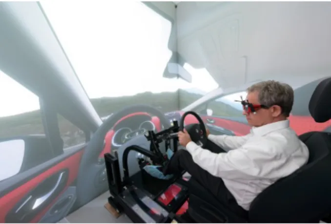
Figure 1 - Renault’s High Performance CAVE with controlled driver station
2. PERCEPTION OF MOVEMENT
2.1. Simulation sickness
If driving simulation and VR are using the same technics they share the same or similar difficulties in rendering movements of the observer in the virtual environments. The worst case is when the observer/driver is turning while driving or moving using a control device (ex. Joystick) in a CAVE or in a static driving simulator. This is due to the visuo-vestibular conflict, due to the discrepancies perceived by the human visual and vestibular systems induce the so-called simulation sickness [3] as the observer/driver may see rotations not perceived by the inner ears.
Another cause is the transport delay, the delay between the action and the corresponding rendering cues. This transport delay depends on the acquisition of observer/driver actions and movements (especially head movements), image frequency rate and motion rendering and may create strong perceptual discrepancies [4]. When observing an image computed in function of head movements, small delays may induce nausea as the Vestibular Ocular Reflex (VOR), which is responsible of eye fixations, is very quick, about 20ms [5]. When driving, these effects may be smaller than for passengers or passive observers as the efferent copies of information given by steering wheel, pedals or other control devices help the driver to anticipate the movement [6].
To avoid simulation sickness, transport delay should be limited to 50 ms in driving simulation [7], 20 ms using HMDs and CAVEs or head slaved or HMD based driving simulators because of the rapidity of the VOR reflex.
Other factors may play a role, as expectations based on previous experiences [8] or any other physiological parameters which influences postural stability. One way to deal with simulation sickness is to provide an acceptable face value of motion, for example by reducing sensory conflicts generating generic proprioceptive cues.
2.2. Perception of distance, speed and acceleration at scale 1:1
Correct perception of speed and acceleration in driving simulation is crucial for automotive experiments for Advances Driver Aid System (ADAS) experiments as vehicle behavior has to be simulated correctly and anywhere where the correct mental workload is an issue as real immersion and driver attention is depending on it [9].
Speed perception is depending on the visual field of view, in part because of the role of peripheral field of view in motion perception by the human visual system and partly because of the corresponding generated immersion level and probably on other parameters, such as steering wheel force feedback and overall CGI quality [10]. The correct perception of accelerations requires the use of motion platform, which makes driving in a CAVE difficult, especially with rear projection floor, allowing only limited payload.
Correct perception of distances and object size is also crucial using HMDs or CAVEs (Figure 2), especially as their use is frequently involving digital mockup validation for design, architecture or interior and exterior lighting. Early VR validation studies showed already differences in distance and scale 1:1 perception between VR and real life conditions [11]. One of the most important visual depth cues is motion parallax and its role was shown real, virtual environments [10] [13] [14]. Nevertheless, the precise role of binocular convergence [15][16] and cognitive factors [17] are still to be further clarified both for scale 1:1 and distance perception.
2.3. User paradigm
Using Renault’s high-performance CAVE, users require for a number of use-cases, especially for vehicle architecture and visual ergonomics studies, driving in a digital mock-up in a virtual environment, which is usually a duplicate of an existing real and well-known environment. In order to ensure an efficient use of the CAVE for these experiments and based in previous observations in the use of driving simulation experiments [14], [14], [14], user experimentation initiated to identify the limits of possible vehicle movements, in order to keep the users in acceptable and comfortable driving conditions. A specific experimentation seemed useful in regard of the visual performances of Renault’s high performance CAVE in terms of resolution, frequency, field-of-view, etc. (see section 3.1), which may have an impact on the visuo-vestibular effect. Furthermore, as in the majority of use-cases drivers are passive, simulation sickness effects may be reinforced [14].
For the planned experiment, low and high level speed and acceleration thresholds were induced, thanks to the experimental driving scenarios settled using the SCANeR Studio © driving simulation software [18] to determine what amplitude of movements is acceptable when driving in a CAVE. Our hypothesis is that the higher the vehicle accelerations, the higher the visuo-vestibular conflict and the more the simulation sickness. In other terms, if the vehicle acceleration is under or close to the vestibular perception threshold, the visuo-vestibular conflict will be non-existent or weak enough to avoid Virtual Reality Induced Symptoms and Effects (VRISE).
Two types of vehicle movements were distinguished in the experiment: translations and rotations. Indeed, physical translational movements and rotational movements are perceived by the different organs in the vestibular system, the otoliths for linear and the semicircular canals for rotations [5].
3. PROTOCOL
3.1. Experimental apparatus
Renault had recently put in use its high performance IRIS (Immersive Room and Interactive System) CAVE™, a 5 sided virtual reality room with a combined resolution of 70 M pixels, distributed over sixteen 4K projectors and two 2K projector as well as an additional 3D HD collaborative power wall. Images of the studied vehicle are displayed in real time thanks to a cluster of 20 HP Z800 computers with 24 Go RAM and 40 nVidia Quadro 6000 graphics boards. The experiment was conducted using Renault’s SCANeR Studio © real time driving simulation software. The image generation frequency with SCANeR in IRIS was 60 Hz with a very detailed town environment. Head tracking was performed with an ART 8-camera infrared tracking system running at 60Hz. A driver station with controlled and measurable seat, steering wheel and driver body position was used for passive driving sessions.
3.2. General purpose
The aim of the experiment was to determine the impact of two factors on motion sickness: longitudinal accelerations and yaw rotations. Thus we built 2 scenarii to study these factors, in which the subjects are in passive driving conditions.
2.5 2 1.5 "Max accel 0.44 m/s2 -Max accel 2.2 m/s2 10 12 14 16 18 20 22 24 26 Time [sec]
Subjects were split into two groups, one group per scenario. And for each study, we compared two conditions: a low-level and a high-low-level stimulus. So every subject had to perform the two conditions of his or her case. In order to have no interference between the conditions, we asked subjects to perform the two conditions on two separate days. In order to avoid order effects, half of the subjects of each group performed the low-level stimulus condition first, and the other half performed the high-level stimulus condition first.
3.3. Longitudinal acceleration study
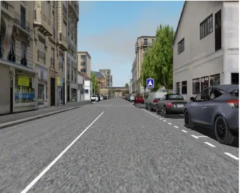
The first scenario takes place on a straight road (Figure 2). The longitudinal speed of the vehicle was controlled to generate a succession of longitudinal accelerations and decelerations. The complete motion of the controlled vehicle is obtained thanks to
MADA, Renault’s vehicle dynamics model.
Figure 3 presents the obtained vehicle acceleration profile. This profile was repeated 8 times by subject for a total duration of 128 seconds.
Figure 2 – Screenshot of the straight road used for the first scenario (longitudinal acceleration study)
Figure 3 – Acceleration profile of the vehicle (repeated 8 times) for the first scenario (longitudinal acceleration study)
Table 1 presents the two proposed levels of stimulus for this first scenario, generating 0.04g and 0.2g acceleration levels:
_r -20 -250 -- -Travel at 12 km /h - Travel at 40 km /h 100 200 300 400 500 600 700 800 Travelled Distance [m] 15 10 -15 -20 -- -Travel at 12 km /h - Travel at 40 km /h 100 200 300 400 500 600 700 800 Travelled Distance [m]
Low-level stimulus High-level stimulus
Longitudinal speed 8 km/h 40 km/h
Longitudinal acceleration 0.44 m/s² 2.2 m/s²
Table 1 – Levels of stimulus for the longitudinal acceleration study
3.4. Rotational (yaw) motion study
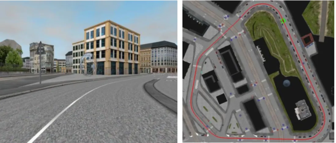
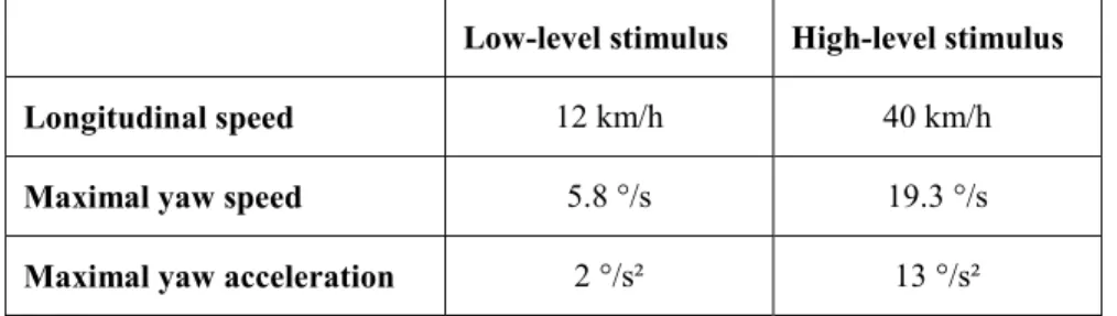
For the second scenario, a succession of straight and curved roads (curvature radius of 30 m, Figure 4) was used. For the two levels of stimulus, the same road was used but at different speeds. Thus the induced yaw speed and acceleration are different. Figure 5 presents these yaw speed and acceleration, given by our vehicle dynamics model (MADA). Table 2 presents the two levels of stimulus for this second scenario with 2°/s2 and 13°/s2.
Figure 4 – Presentation of the curved road used for the second scenario (yaw motion study)
Low-level stimulus High-level stimulus
Longitudinal speed 12 km/h 40 km/h
Maximal yaw speed 5.8 °/s 19.3 °/s
Maximal yaw acceleration 2 °/s² 13 °/s²
Table 2 - Levels of stimulus for the yaw rotation study
The vehicle yaw rotation speed can be simplified by the formula = , where V is the longitudinal speed and RC the curvature radius. As the curvature radius of the trajectory is the same in both conditions and only the longitudinal speed varies (12 km/h and 40 km/h), this is why we can observe that the rotational speeds are proportional between the 2 conditions (Figure 5, left).
3.5. Measures
Before performing the driving sessions, subjects had to read information notices and complete questionnaire about themselves and their use of virtual reality and driving simulation tools. To measure the motion sickness, the Simulator Sickness Questionnaire (SSQ [19] was used. Subjects had to fill it before and after the driving to compare the results. Postural stability was also measured, as some studies show possible relation with motion sickness [20]. The Techno-Concept Stabilotest platform is a professional stabile-metric platform, used by podiatrists and allowing recording the center of gravity projection on the floor. The system can provide the area of the smallest ellipse surrounding the trajectory of the center of gravity. Two records were performed: one before and one after the driving session. The evolution of the ellipse area between the subjects was consequently measured for every subject. Each record lasted 50 seconds during which subjects were asked to stand as immobile as possible while keeping their arms along their body, keeping their eyes open and fixing a constant point in front of them.
4. RESULTS
4.1. Longitudinal acceleration study
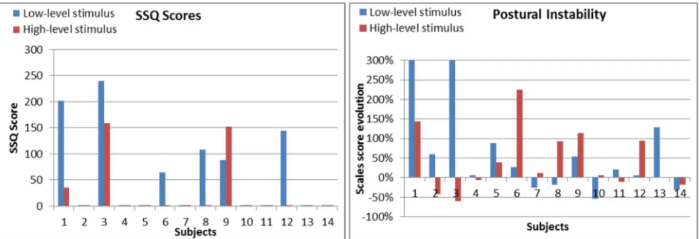
Figure 6 presents the results of the longitudinal acceleration study. In both graphs, blue bars correspond to the low-level stimulus (0.44 m/s²) and red bars to the high-level stimulus (2.2 m/s²). The left graph presents the postural instability evolution (in percentage) between before and after the driving. The graph on the right presents the SSQ scores.
Low -level stimulus High -level stimulus 300 250 d 200 ó Ñ 150 C m
^
100 50 0 SSQ Scores 1 2 3 4 5 6 7 8 9 10 11 12 13 14 SubjectsLow -level stimulus High -level stimulus 300% e25°% 0 to 200% 0 150% d 22100% x 50% d To 0% vt -50% -100% Postural Instability
L
14
1..,J,J,,,,.... i
ti1
4 5 6 8 9 11 12 13i4
SubjectsLow -level stimulus High -level stimulus 250 200 d 150 9; 100 50
SSQ
Scores 1 2 3 4 5 6 7 8 9 10 11 12 13 14 Subjects Low-level stimulusPostural
Instability
High -level stimulus200% 150% 100% 50% 0% -50% -100%
IIL1ui
I
1 4 5 6 7 89
11 1!7
14 SubjectsFigure 6 – SSQ scores and postural instability evolution for the two longitudinal acceleration levels
We can notice that the majority of subjects weren’t sick in any condition. On the other hand, subjects who experienced VRISE, the trend is opposite to our initial hypothesis: subjects have higher SSQ values with low speed values than with higher values Z=-1.84, p<0.06. A possible explanation is that VRISE is also induced by incoherencies induced by the transport delay, the lag between head motions and the corresponding computed images, which is more observable at low speed.
These results suggest that most subjects are accepting relatively high longitudinal accelerations, up to 0.2g, for short time periods, that is during a few seconds. On the contrary other incoherencies, due to high transport delays for example may have more severe effects on driver sickness or uneasiness, especially at low speeds.
There was no difference in postural instability between the two conditions. Furthermore, the measured postural instability values are not correlated to the SSQ scores.
4.2. Rotational (yaw) motion study
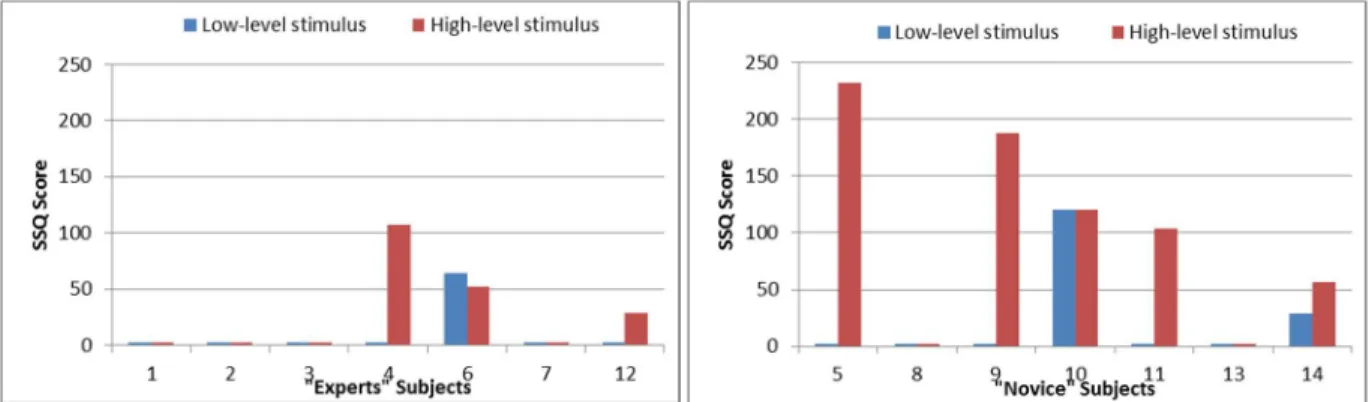
Figure 7 presents the results for the rotational (yaw) motion study. In both graphs, blue bars correspond to the low-level stimulus and red bars to the high-level stimulus. The left graph presents the postural instability evolution (in percentage) between before and after the driving. The graph on the right presents the SSQ scores.
250 200 ó 150 Li a100 50 0
Low -level stimulus High -level stimulus
'
i
1 2 3Experts4Subjects 7 12 250 200 c 150 100 50 0Low -level stimulus High -level stimulus
5 g INovicelSubject 1 13 14
The ANOVA performed on the SSQ Scores showed a significant effect of rotation speed (F(2,14)=4.57, p<.05), the higher acceleration levels induced significantly higher SSQ values, showing a strong VRISE effect with the higher rotational accelerations.
There was no difference in postural instability between the two conditions for rotational motions either. Furthermore, the measured postural instability values are not correlated to the SSQ scores.
Figure 8 - SSQ scores for the two rotational (yaw) motion levels – expert subjects on the left and novice subjects on the right
With subjects split into two groups, expert and novice subjects according to personal questionnaire answers, the ANOVA performed on the SSQ Scores showed a strong VRISE (F(2,7)=4.69, p=0.05) for novice subjects with the higher rotational motions, while experienced subjects have not experienced almost any simulation sickness (see Figure 8).
5. CONCLUSION
Results show that for rotational motion naïve subjects experienced significantly higher SSQ values when the acceleration values were higher (up to 13°/s2) comparatively to low levels (2°/s2) and with the lower level motions they have not experienced significant VRISE (nevertheless still two subjects experienced a slight uneasiness without a disturbing driving effect) and often with zero SSQ values. These naïve subjects seemed to experience an easy ride with the low, about 2°/s2 values, though were uneasy with the higher, 13°/s2 values.
Results also show that the group of experienced subjects had low SSQ values in the two different sessions, independently on the acceleration values and had always zero or very low SSQ values. Thus it would seem that with experienced subjects, such as gamers or VR specialists, these rotational VRISE are low but for naïve subjects low rotational motion levels are required to avoid significant VRISE.
In addition we can also observe that SSQ and postural stability values are not correlated in our experiments. Previous studies have already shown that the relationship between motion sickness and postural stability may vary according to motion characteristics [21], especially in driving situations where even negative correlation may be observed [22], well in accordance with our findings.
6. REFERENCES
[1] Kemeny A., “From Driving Simulation to Virtual Reality”, VRIC 2014, Laval Virtual, pp. AE2, 1-5 (2014) [2] Shermann W. R. and Craig A. B.,[Understanding Virtual Reality], Morgan Kaufmann, San Francisco (2003)
[3] Kennedy, R. S., Lane, N. E., Grizzard, M. C., Stanney, K. M., Kingdon, K., & Lanham, S., “Use of a motion history questionnaire to predict simulator sickness”, Proceedings of the Sixth Driving Simulation Conference, DSC2001, France, pp. 79-89 (2001)
[4] Kemeny A., “Recent developments in visuo-vestibular restitution of self-motion in driving simulation”, Proceedings of the Driving Simulation Conference, Sophia Antipolis, pp.15-18 (2001)
[5] Berthoz A., [The Brain's Sense of Movement], Harvard University Press (2002)
[6] Dagdelen M., Reymond G., Kemeny A., “Analysis of the visual compensation in the Renault driving Simulator”, Proceedings of the Driving Simulation Conference, Paris, pp 109-119 (2002)
[7] Allen R. W., Jex H. R. “Driving simulation, mechanization and application”, SAE paper, n° 800448 (1980) [8] Reason J. T., Brand J., [Motion Sickness], London: Academic Press (1975)
[9] Barthou A., Kemeny A., Reymond G., Merienne F., Berthoz A., “Driver trust and reliance on a navigation system: effect of graphical display”, In A. Kemeny, F. Mérienne, S. Espié (Eds.), Trends in Driving Simulation Design and Experiments. Les Collections de l'INRETS, pp. 199-208 (2010)
[10] Panerai F., Droulez J., Kelada J-M., Kemeny A., Balligand E., Favre B., “Speed and safety distance control in truck driving: comparison of simulation and real-world environment”, Proceedings of the Driving Simulation Conference, Sophia Antipolis, pp.21-32 (2001)
[11] Loomis, J. M. and Knapp, J. M., “Visual perception of egocentric distance in real and virtual environments”, In Virtual and Adaptive Environments, eds. L.J. Hettinger and M. W. Haas, Erlbaum, Mahwah NJ., pp. 21-46 (2003)
[12] Rogers B., Graham M., “Motion parallax as an independent cue for depth perception”, Perception 8, pp. 125-134 (1979)
[13] Panerai, F., Cornilleau-Peres, V. and Droulez, J., “Contribution of extraretinal signals to the scaling of object distance during self-motion”, Percept Psychophys. 64, pp.717-731 (2002)
[14] Kemeny, A. and Panerai, F., “Evaluating perception in driving simulation experiments”, Trends in Cognitive Sciences 7, pp. 31-37 (2003)
[15] Paillé D., Kemeny A., Berthoz A., “Stereoscopic Stimuli are not used in Absolute Distance Evaluation to Proximal Objects in Multi-Cue Virtual Environment”, Proceedings of SPIE Vol. 5664, pp. 596-605 (2005) [16] Kemeny A., Combe E., Posselt J., “Perception of Size in Vehicle Architecture Studies”, Proceedings of the 5th
Intuition International Conference, Torino, Italy (2008)
[17] Glennerster A., Tcheang L., Gilson S. J., Fitzgibbon A. W., Parker A. J., “Humans ignore motion and stereo cues in favor of a fictional stable world”, Current Biology 16(4), pp. 428-432 (2006)
[18] Kemeny, A., “A Cooperative Driving Simulator”, Proceedings of the International Training and Equipment Conference, London, May 1993, pp.67-71, (1993)
[19] Kennedy R. S., Lane N. E., Berbaum K. S., Lilienthal M. G., “Simulator Sickness Questionnaire: an enhanced method for quantifying simulator sickness”, The International Journal of Aviation Psychology, 3(3), pp. 203-220 (1993)
[20] Riccio G.E., Stoffregen T.A., “An ecological theory of motion sickness and postural instability”, Ecological Psychology 3, pp. 195-240 (1991)
[21] Bos J., “Nuancing the relationship between motion sickness and postural stability”, Displays, 32, pp. 189-193 (2011)
[22] Reed-Jones R.J., Vallis L.A., Reed-Jones J.G., Trick L.M., “The relationship between postural stability and virtual environment adaptation”, Neuroscience Letters 435, pp. 204-209 (2008)