Model order reduction of quasi-static problems based on POD and PGD approaches

(1)

Science Arts & Métiers (SAM)

is an open access repository that collects the work of Arts et Métiers Institute of

Technology researchers and makes it freely available over the web where possible.

This is an author-deposited version published in: https://sam.ensam.eu Handle ID: .http://hdl.handle.net/10985/7234

To cite this version :

Thomas HENNERON, Stéphane CLENET - Model order reduction of quasi-static problems based on POD and PGD approaches - The European Physical Journal Applied Physics n°5, p.1-7 - 2013

Any correspondence concerning this service should be sent to the repository Administrator : archiveouverte@ensam.eu

(2)

(will be inserted by the editor)

Model order reduction of quasi-static problems based on POD

and PGD approaches

Thomas Henneron1 a _{and St´}_{ephane Cl´}_enet2

1 _{L2EP, Universit´}_{e Lille 1, 59655 Villeneuve dAscq, France}

2 _{L2EP, Arts et M´}_{etiers ParisTech, 59046 Lille, France}

Received: date / Revised version: date

Abstract. In order to reduce the computation time of a quasi-static problem solved by the finite element

method, methods of model order reduction can be applied. In this context, two approaches, the Proper Orthogonal Decomposition and the Proper Generalized Decomposition, are applied to the vector poten-tial formulation used to solve the quasi-static problem. The developped methods are compared on an academic example.

1 Introduction

In quasi-static problems, the distributions of the magnetic and electric fields depend on time. By using a numerical approach, the Maxwell equations are discretized simul-taneously in the space and the time domains. To solve this kind of problem, the finite element method is com-monly used to approximate the distribution of the fields in the space domain. The time domain can be discretised by an implicit or explicit Euler scheme or any time-stepping schemes. If the mesh of the space domain is fine and a small time step is used, the computation time can be sig-nificant. To tackle this issue, an alternative is to use model order reduction methods. These approaches consist in ex-panding the solution of the initial problem in a reduced basis. In the litterature, several approaches have been de-veloped, we can distinguish the a-priori and a-posteriori methods. In this work, two methods of model order re-duction are applied to solve quasi-static field problems. The first method is the Proper Orthogonal Decomposition (POD) approach which is an a-posteriori method [1]. It consists in performing a projection onto the reduced basis of the space domain. In the discrete domain, the Snapshot approach is mainly used to determine the discrete projec-tion operator [2]. In computaprojec-tional electromagnetics, the POD method has been applied, for example, to study the behavior of magnetic core with non linear static hysteresis [3] or to solve an electroquasistatic field problem [4]. The second approach presented is the Proper Generalized De-composition (PGD) method which is an a-priori method. This is based on the separated representation of the solu-tion, as for example, in function of time and space [5][6][7]. In computational electromagnetics, the PGD method has been applied to study a fuel cell polymeric membrane model [8], the skin effect in a conducting domain [9][10]

a

Present address: thomas.henneron@univ-lille1.fr

or a soft magnetic composite microstructure [11]. These two methods of model order reduction are investigated to solve a quasi-static problem using the vector potential for-mulation. In a ﬁrst part, the quasi-static problem and the vector potential formulation are presented. In the second part, the POD and PGD approaches are developped. Fi-nally, a 3D academic example is studied with both meth-ods. The results are compared with those obtained by a more classical approach, fully discretised in the time and space domains.

2 Maxwell’s equations and vector potential

formulation

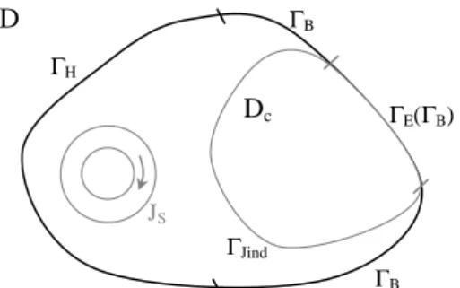
Let us consider a domain D of boundary Γ (Γ = ΓB∪ ΓH

and ΓB ∩ ΓH = ∅). In D, a conducting domain Dc of

boundary Γc(Γc= ΓJ ind∪ΓEand ΓE⊂ ΓB) is introduced

(Fig. 1). JS ΓB ΓH ΓE(ΓB) ΓJind D Dc ΓB

(3)

2 T. Henneron and S. Cl´enet: Model order reduction of quasi-static problems based on POD and PGD approaches

The quasi-static ﬁeld problem can be represented by Maxwell’s equations without the displacement current,

curl E(x, t) =−∂tB(x, t), (1)

curl H(x, t) = Jind(x, t) + Js(x, t), (2)

div B(x, t) = 0, (3)

div (Jind(x, t) + Js(x, t)) = 0 (4)

with B the magnetic flux density, H the magnetic field, E the electric field, Jsthe known current density flowing

through the stranded inductors and Jindthe eddy current

density in the conducting domain. To take into account the material behavior, the constitutive relations between the ﬁelds B and H and the ﬁelds Jind and E must be

considered. In the linear case, we have

B(x, t) = µ0µrH(x, t), (5)

Jind(x, t) = σE(x, t) (6)

with µ0 the magnetic permeability of the vacuum, µrthe

relative permeability and σ the electric conductivity. To impose the unicity of the solution, boundary conditions must be added

H(x, t)× n = 0 on ΓH, (7)

B(x, t)· n = 0 on ΓB, (8)

E(x, t)× n = 0 on ΓE, (9)

Jind(x, t)· n = 0 on ΓJind (10)

with n the outward unit normal vector.

To solve the previous problem, the A_∗formulation can be used. A magnetic vector potential A_∗(x, t) is deﬁned in the whole domain by using (1) and (3)

B(x, t) = curl A_∗(x, t) , E(x, t) =−∂tA_∗(x, t) (11)

and A_∗(x, t)× n = 0 on ΓB.

Combining the previous relations and the behavior laws in (2), we obtain the vector potential formulation of the problem which must be solved in D× [0, T ] with T the length of the time interval. The weak form to be solved is then written ∫ T 0 ∫ D 1 µcurl A∗(x, t)· curl A ′_(x) +σ∂tA∗(x, t)· A′(x)dDdt = ∫ T 0 ∫ D Js(x, t)· A′(x)dDdt (12)

with A′(x) a test function deﬁned on the same space as A_∗. In the 3D case, the potential A_∗(x, t) is semi-discretised in space by using the edge elements:

A_∗(x, t) =

Ne ∑

i=1

Ai(t)wai(x) (13)

with wai the edge shape function associated with the

i -th edge, Ai(t) a function of time and Ne the number

of edges. We denote by AD(t) the vector of components

(Ai(t))1_≤i≤Ne. Then a system of coupled ordinary diﬀer-ential equations has to be solved

M AD(t) + N dAD(t) dt = F (t) (14) with Mi,j= ∫ D 1 µcurl wai(x)· curl waj(x)dD, Ni,j= ∫ Dc σwai(x)· waj(x)dDc, Fi(t) = ∫ D Js(x, t)· wai(x)dD.

Generally, to solve (14) in the time domain, an Euler scheme is used. In the following, the known current density Js in the stranded inductors is expressed by a separated

representation

Js(x, t) = N (x)i(t) (15)

with N (x) the source ﬁeld and i(t) the evolution of the current versus the time that is supposed to be known.

3 Model order reduction

The Proper Orthogonal Decomposition and the Proper Generalized Decomposition methods are based on a sep-arated representation of space and time functions of the potential A_∗(x, t) A_∗(x, t)≈ M ∑ n=1 Rn(x)Sn(t) (16)

with Rn(x) deﬁned on D, Sn(t) deﬁned on [0, T ] and M

the number of modes taken into account for the approxi-mation of A_∗(x, t). The aim of the POD and PGD meth-ods is to ﬁnd the ”best” separated representation with M functions.

3.1 Proper Orthogonal Decomposition

With the POD method [1], we consider that the functions Rn(x) are an orthogonal basis, that is

∫

D

Ri(x)· Rj(x)dD = 0 if i̸= j. (17)

The functions Sn(t) can be expressed from the projection

of A_∗(x, t) on the basis of functions Rn(x) such that

Sn(t) =

∫

D

A_∗(x, t)· Rn(x)dD. (18)

To determine the set of functions Rn(x), we aim at

min-imizing the quantity ∥A∗(x, t)− M ∑ n=1 Rn(x)Sn(t)∥2 (19) =∥A_∗(x, t)− M ∑ n=1 ( ∫ D A_∗(x, t)· Rn(x)dD)Rn(x)∥2

(4)

To determine a discrete representation of the functions Rn(x), the Snapshot method can be used [2]. In a ﬁrst

step, the system (14) is solved for the ﬁrst M time steps (called Snapshots). The M vectors of AiDobtained at each

time step are gathered in a matrix AS of size Ne× M. In

the discrete domain, (18) and (19) can be written

P = ASR, (20)

AS= P ASr (21)

with ASr the matrix of the Snapshot in the reduced

ba-sis, R a matrix whose column i corresponds to the discrete representation of the function Ri, Ptthe discrete

projec-tion operator between the values of A_∗ in the basis of the Ne edge functions and the reduced basis. In order to

determine the expression of P , a Singular Value Decom-position (SVD) is applied to the matrix of Snapshots such that AS = V ΣWt with Σ the diagonal matrix of the

singular values, V and W the orthogonal matrices of the left and right singular vectors. By combining (20), (21) and the SVD of AS, we have

AS= V ΣWtRASr. (22)

By ﬁxing R = W , since W is orthogonal W Wt= I, the previous equation can be simpliﬁed such that

AS = V ΣASr. (23)

By identification, the expression of P can be defined such that P = V Σ. Another approach to obtain the expression of P can be carried out by the calculation of the SVD of the correlation matrix defined by At_SAS. The reduced

matrix system can be deduced by using the operator P in (14) to obtain MrAr(t) + Nr dAr(t) dt = Fr(t) (24) with Mr= PtM P , Nr= PtN P and Fr(t) = PtF (t).

The size of the matrices Mr and Nr and the vectors

Fr and Ar depend on the number of Snapshots that is

generally much smaller than the number of edges of the mesh. To obtain the solution on [0, T ], the reduced matrix system is solved all time steps. For each time step, the solution on the original mesh AD(t) can be retrieved from

the solution Ar(t) of the reduced model by

AD(t) = PtAr(t). (25)

3.2 Proper Generalized Decomposition

With the PGD approach, the weak formulation deﬁned by (12) is considered. To compute the functions Rn(x)

and Sn(t), an iterative enrichment method is used. The

couple (Rn(x), Sn(t)) is calculated regarding the previous

couples (Ri(x), Si(t)) with i∈ [1, n − 1]. In this case, the

test function A′ can be written such that

A′(x, t) = R′n(x)Sn(t) + Rn(x)Sn′(t) (26)

with R′_n(x) and S_n′(t) the test functions deﬁned in the same spaces as Rn(x) and Sn(t) respectively. Each

cou-ple (Rn(x), Sn(t)) is calculated by solving iteratively two

equations determined from (12). First, we suppose that Rn(x) is known. Then, the function R′n(x) vanishes in

(26) and the test function A′ is equal to Rn(x)Sn′(t).

Equation (12) is solved in order to determine the func-tion Sn(t). This can be rewritten

∫ D 1 µcurlRn(x)· curlRn(x)dD ∫ T 0 Sn(t)· Sn′(t)dt + ∫ D σRn(x)· Rn(x)dD ∫ T 0 ∂tSn(t)· Sn′(t)dt = ∫ D N (x)· Rn(x)dD ∫ T 0 i(t)· Sn′(t)dt − n−1 ∑ i=1 ∫ D 1 µcurlRi(x)· curlRn(x)dD ∫ T 0 Si(t)· Sn′(t)dt − n−1 ∑ i=1 ∫ D σRi(x)· Rn(x)dD ∫ T 0 ∂tSi(t)· Sn′(t)dt. (27)

One can note that the previous equation is a weak form of the following Ordinary Diﬀerential Equation

ARSn(t) + BR dSn(t) dt = CS(t) (28) AR= ∫ D 1 µcurlRn(x)· curlRn(x)dD BR= ∫ D σRn(x)· Rn(x)dD CS(t) = i(t) ∫ D N (x)· Rn(x)dD − n_∑−1 i=1 Si(t) ∫ D 1 µcurlRi(x)· curlRn(x)dD − n_∑−1 i=1 dSi(t) dt ∫ D σRi(x)· Rn(x)dD.

Secondly, we compute the function Rn(x) assuming that

Sn(t) is known. In this case, the function S′n(t) vanishes

in (26) and the test function A′ is equal to R′_n(x)Sn(t).

To determine Rn(x), the relation (12) is solved with these

conditions. This corresponds to ∫ T 0 Sn(t)· Sn(t)dt ∫ D 1 µcurlRn(x)· curlR ′ n(x)dD + ∫ T 0 ∂tSn(t)· Sn(t)dt ∫ D σRn(x)· R′n(x)dD = ∫ T 0 i(t)· Sn(t)dt ∫ D N (x)· R′_n(x)dD − n₋₁ ∑ i=1 ∫ T 0 Si(t)· Sn(t)dt ∫ D 1 µcurlRi(x)· curlR ′ n(x)dD − n₋₁ ∑ i=1 ∫ T 0 ∂tSi(t)· Sn(t) ∫ D σRi(x)· R′n(x)dDdt. (29)

(5)

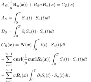
The equation is also a weak form of a Partial Derivative Equation that can be written under the form

AS( 1 µRn(x)) + BSσRn(x) = CR(x) (30) AS = ∫ T 0 Sn(t)· Sn(t)dt BS = ∫ T 0 ∂tSn(t)· Sn(t)dt CR(x) = N (x) ∫ T 0 i(t)· Sn(t)dt − n−1 ∑ i=1 curl(1 µcurlRi(x)) ∫ T 0 Si(t)· Sn(t)dt − n−1 ∑ i=1 σRi(x) ∫ T 0 ∂tSi(t)· Sn(t)dt.

The solution (Rn(x), Sn(t)) veriﬁes the ODE (28) and the

PDE (30). This solution is obtained by an iterative proce-dure. In our case, we assure that Sn(t)0= 1 on [0, T ], then

solving (30) we obtain Rn(x)0. Solving (28) taking Rn(x)

= Rn(x)0, we obtain Sn(t)1and then the equation (28) is

solved with Sn(t) = Sn(t)1 and so on. This procedure is

stopped once the diﬀerence between two consecutive iter-ates is suﬃciently small. If we denote by (Rn(x)j, Sn(t)j)

and (Rn(x)j−1, Sn(t)j−1) the couples of functions

deter-mined at the iteration j and j− 1.

The convergence proof of the separated solution rep-resentation methods has been given in [12]. Our problem does not belong to this class of problem. However, even though the proof is not given, our problem is similar to other ones which have been solved with the PGD approach and for which no convergence proof has been given [13]. In term of solution, the ODE formulation (28) can be easily solved by the Euler implicit scheme. The functions Sn(t)

and i(t) are discretised in each time step. The weak for-mulation (29) is solved to determine the functions Rn(x),

for example, by using the ﬁnite element method. The func-tions Rn(x) and N (x) are discretised in the edge shape

function space with the same boundary conditions as A_∗ and in the facet shape function space respectively [14].

4 Application

As a 3D application example, a stranded inductor located between two conducting plates is considered. Due to the symmetries of the device, only one eighth of the system has been modeled (Fig. 2). The inductor is supplied by a sinusoidal current with a magnitude equal to 1A and a frequency of 20kHz. The number of turns of the inductor is equal to 100. The relative magnetic permeability of the conducting plate is ﬁxed to 1 and its electrical conductiv-ity to 10kS/m. The 3D spatial mesh has 14970 nodes and 80199 tetrahedrons. The problem has been solved using the POD and PGD approaches applied to the A_∗ formu-lation. In order to evaluate the eﬃciency of the proposed

models, the A_∗ formulation has been solved using a time stepping Finite Element Method. This approach will be considered in the following as the reference.

Fig. 2. Example of application

In the following, we denote by MPOD, MPGD and MREF the models obtained from the POD, PGD and clas-sic approaches.

4.1 Influence of the number of modes on the global values

The length of the time interval is fixed to 0.1ms with 60 time steps. In order to evaluate the influence of the number of modes M on the global values, the evolutions of Joule losses versus the time obtained from MPOD and MPGD are compared with those computed from MREF in Fig. (3) and (4) respectively. We can observe that the number of modes influences the evolution of the Joule losses for both methods. To estimate the convergence versus the number of modes of these curves, an error estimator ϵ(P j)is defined such that

ϵ(P j)=

∥P jref− P jest∥2 ∥P jref∥2

(31)

with P jrefand P jestthe vectors of Joule losses for all time

steps obtained from MREF and MPOD or MPGD. Fig-ure (5) presents the evolution of ϵ(P j) versus the number of modes. The curves of error converge until zero. With MPOD the convergence is faster than with the MPGD. To obtain an error inferior to 0.1 percent, 5 modes are required with the MPOD and 12 with the MPGD.

In the case of MPGD, the evolutions of the functions Sn(t) in the time domain are determined. In ﬁgure (6), the

evolutions of the functions Sn(t) for the four ﬁrst modes

are presented. A transient state can be observed on all curves. This transient state can also be observed on the evolution of the Joule Losses (Fig. (4)).

(6)

0 0.2 0.4 0.6 0.8 1 1.2 1.4 1.6 1.8 2 0 0.01 0.02 0.03 0.04 0.05 ref 2 3 4 t(ms) Pj(W) _ref M=2 M=3 M=4

Fig. 3. Joules losses obtained from the POD method

0 0.5 1 1.5 2 2.5 0 0.01 0.02 0.03 0.04 0.05 ref 2 4 7 10 12 t(ms) Pj(W) _ref M=2 M=4 M=7 M=10

Fig. 4. Joules losses obtained from the PGD method

0 10 20 30 40 50 60 0 2 4 6 8 10 12 POD PGD Nb Mode

ε

Pj(%) PGD POD

Fig. 5. Error on the Joules losses versus the number of modes

for both methods

-1,5 -1 -0,5 0 0,5 1 1,5 2 0 0,02 0,04 0,06 0,08 0,1 1 2 3 4 t(ms) 10-13 S1(t) S2(t) S3(t) S4(t)

Fig. 6. Evolution of the four first modes Sn(t)

4.2 Influence of the number of modes on the fields distribution

As the vector potential is approximated by a sum of con-tribution associated with each mode, it is possible to give a distribution of the magnetic ﬂux density and of the eddy

current density for each mode. For MPGD, the figures (7) and (8) present the distribution of B on a section P pre-sented in Fig. (2) for the first and the second mode. For the POD approach, the figures (9) and (10) present the distributions of B for the first and second mode.

Fig. 7. Distribution of B(T ) for the first mode given by MPGD

Fig. 8. Distribution of B(T ) for the second mode given by

MPGD

(7)

Fig. 10. Distribution of B(T ) for the second mode given by

MPOD

Since the reduced basis are differents, the distributions of B obtained from MPOD and MPGD are not similar for each mode. With MPGD, for the first mode, it seems that the distribution does not take into account the effect of the conducting plate. For the second mode, the distribution is close to the reaction magnetic field distribution due to the eddy current density. With MPOD, for the first mode, the distribution takes into account the eddy current in a conducting plate. With the second mode, we observe a reaction magnetic flux density due to the eddy current density.

For the global distribution of the magnetic ﬂux density obtained with MPOD and MPGD, the results are close to the one computed with MREF.

4.3 Computation time

In terms of computation time, with a length of the time interval of 0.1ms and 60 time steps, the MREF requires 5min7s to solve the numerical problem. For MPOD, the computation time is of 1min50s, this time takes into ac-count the solution of original model (14) with 5 snapshots and 60 solutions of the reduced model (24). The size of the matrix system to solve is reduced, thus the computation time requires to solve the numerical problem (24) by us-ing an iterative method is small compared to MREF. We should mention that the calculation of the matrices Mr

and Nr and the vector Fr which could be cumbersome

is not undertaken. In the iterative procedure by using a conjugate gradient method, only matrix-vector products are required, in the algorithm of the method, the prod-uct MrXj with Xj the vector of the approximated

so-lutions at the j -th iteration is calculated by PtM P Xj.

In the linear case, the calculation of the product MrXj

without using an explicit expression of Mr is not

nec-essarily the most eﬃcient. In the non linear case, it is not possible to determine Mr explicitly and the

calcula-tion of PtM P Xj is required because M is a function of

the solution [15][16]. With MPGD, the computation time is of 11min, this time takes into account the determina-tion of the funcdetermina-tions Rn(x) and Sn(t) associated with 15

modes. Each mode requires from 4 to 18 iterations to be

determined. Then, 83 numerical solving of (28) and (29) are necessary. In term of computation cost, the numerical solving of (29), which is close to this of MREF, is more important than the solving of (28) due to the number of unknowns in the space domain (mesh) much greater than the number of time steps. We can note that the original PGD method presented in this article can be improved in order to reduce the number of modes with regard to a given precision [6] [7]. To study the influence of the num-ber of time steps on the computation time, a length of the time interval to 0.2ms with 120 time steps is consid-ered. The computation time require for MREF, MPOD and MPGD is of 10min4s, 3min4s and 9min56s respec-tively. As the number of time steps is multiplied by two, so is the computation time for MREF. For MPOD, as the computation cost of the solution of the original model for 5 snapshots is significant compared with this of the re-duced model, the computation time is not multiplied by two. For MPGD, the computation time is slightly reduced compared with the first study. In fact, the number of nu-merical solving of (28) and (29) required to determine the space and time functions is smaller than for the first study (63 times solving). With MPGD, the computation time is less influenced by the number of time steps.

5 Conclusion

The Proper Orthogonal Decomposition and the Proper Generalized Decomposition method associated with the vector potential formulation has been developed in order to solve a 3D quasi-static ﬁeld problem. On the 3D ap-plication example, it appears that the accuracy of the so-lution obtained from both reduction methods is similar compared with this of a fully described model. With the POD model, the reduction of computation time is signiﬁ-cant. With the PGD model, the computation time is not proportional to the number of time steps. On the studied example, the POD model requires less computation time and number of modes than the PGD model.

References

1. J. Lumley, Atmospheric Turbulence and Wave Propagation, 221 (1967)

2. L. Sirovich, Q. Appl.Math., XLV, 561 (1987) 3. Y. Zhai, IEEE Trans. Magn., 43, 1888 (2007)

4. E. Bergische, M. Cl´emens, IEEE Trans. Magn., 48, 567,

(2012)

5. F. Chinesta, A. Ammar, E. Cueto, Archives of Computa-tional Methods in Engineering, 17, 327 (2010)

6. A. Nouy, Computer Methods in Applied Mechanics and En-gineering, 199, 1603 (2010)

7. A. Ammar, B. Mokdad, F. chinesta, R. Keunings, Journal of Non-Newtonian Fluid Mechanics, 144, 98 (2007)

8. P. Alotto, M. Guarnieri,F. Moro, A. Stella, IEEE Trans. Magn., 47, 1462, (2011)

9. M. Pineda, F. Chinesta, J. Roger, M. Riera, J. Perez, F. Daim, COMPEL, 29, 919, (2010)

(8)

10. T. Henneron, S. Cl´enet, Proceeding of COMPUMAG2011

11. T. Henneron, A. Benabou, S. Cl´enet, IEEE Trans. Magn.,

48, 1218, (2012)

12. A. Ammar, F. chinesta, A. Falco, Archives of Computa-tional Methods in Engineering, 17, 473, (2010)

13. F. Chinesta, P. Ladeveze, E. Cueto, Archives of Computa-tional Methods in Engineering, 18, 395, (2011)

14. A. Bossavit, IEEE Trans. Magn., 24, 74 (1988)

15. T. Henneron, S. Cl´enet, Proceeding of OIPE2012

16. D. Schmidth¨ausler, S. Sch¨ops, M. Clemens, Proceeding of