R. Paulus1, J. Ernst1, B.J. Dewals1,2, P. Archambeau1, S. Erpicum1 and M. Pirotton1 1
Research Unit of Hydrology, Applied Hydrodynamics and Hydraulic Constructions, Department ArGEnCo, Liège University; Chemin des Chevreuils 1 – Bât B52/3, 4000 Liège, Belgium; PH (32) 04-366.90.04; email: [email protected]
2
Belgian Fund for Scientific Research (F.R.S.-FNRS) ABSTRACT
Dam break flow modelling is a major field of research. In order to enable risk analysis in the downstream valleys of dams, 2D numerical simulations are of prime interest. These are based on the conservative set of shallow water equations. Beyond their numerical implementation, the challenge of the computation relies on the ability to handle very huge sets of high-precision data, in order to get the highest possible accuracy, whereas the computational time must remain realistic for simulations carried out on real valleys topography.
In this paper, a simulation on about 2 500 000 cells is presented. Particularly, the results are compared and discussed regarding especially the exploitation of landuse data for the roughness. Beyond the examples of validation, the relevance of the developed methodology appears to be essential in the framework of risk analysis. INTRODUCTION
For almost fifteen years, the HACH unit of Liege University has been studying hydraulic unsteady phenomena, developing therefore numerical and mathematical tools in order to simulate the widest possible range of free surface and pressurized flows (Kerger et al. 2009) with regime transitions. The developed modeling system WOLF enables the simulation of hydrological runoff (spatially distributed and process-oriented) (Archambeau 2006; Khuat Duy et al. 2009); 1D flows (Archambeau 2006) and 2D flows, either as pure hydrodynamics, or coupled with air entrainment, sediment (Dewals et al. 2008), or pollutant transport (Erpicum et al. 2006), or with turbulence models including an original k-! model (Erpicum et al. 2009b). Finally, an optimisation tool, based on Genetic Algorithms (Erpicum 2006) is available. Other functionalities of WOLF include the use of moment of momentum equations, as well as computations considering vertical curvature effects by means of curvilinear coordinates in the vertical plane (Dewals et al. 2006b).
Among all the hydraulic phenomena that are studied within the HACH, dam breaks deserved a particular interest. All around the world, dams are pictured in order to fulfil an increasing demand of hydroelectricity and need of water regulation. In the context of a very demanding management, any dysfunction leads to significant
economic losses and fatalities. The evolution of international guidelines emphasizes the need for risk analysis from the design stage of the dam and during operation of the plant. Numerical computation are therefore used in order to simulate events induced by dam failures scenarios recommended by ICOLD.
Many authors have shown early interest in dam break flow numerical computation (Alcrudo et al. 1992; Bellos and Sakkas ; Fennema and Chaudhry ; Fread 1984; Glaister). Various techniques have been developed to solve the 1D flow equations (Garcia-Navarro et al. 1999). In the early nineties, research was conducted at the University of Liege (Pirotton 1994), leading to a 1D upwind finite element scheme to compute dam break flows on natural topography and to its validation by physical modeling. Nowadays, 2D simulations (which will be presented into further details in this paper) based on the classic fully dynamic shallow water equations have proved their reliability (Dewals et al. 2006a; Dewals et al. 2006c; Erpicum et al. 2004; Erpicum et al. 2009a).
While the challenges of numerical implementation of 2D flow equations are well identified, some specific data features deserve to be examined more deeply, to optimize the computational cost for a fiven need of accuracy.
The accuracy of some of these input data essentially depend on the chosen grid (e.g. topography), whereas some of them rely on empirical knowledge, such as the roughness coefficient. Since the topographic models are nowadays very precise, the macro-roughness of buildings (Figure 2-b) is directly taken into account within the topographic model itself.
The friction coefficient can therefore be selected in accordance with the land cover since the size of the meshes enables to detect precisely different kinds of surfaces (streets, roofs, meadows, forest …).
In this paper, an application of about 2 500 000 cells is presented and analyzed in this new geomatic approach.
The relevance of the developed methodology shows its interest for emergency action planning and comprehensive risk analyses.
MATHEMATICAL AND NUMERICAL MODEL
The two-dimensional model is based on the depth-averaged equations of volume conservation and of momentum conservation, namely the “shallow-water” equations. The large majority of flows occurring in rivers, even highly transient ones such as those induced by dam breaks, are proved to remain shallow everywhere, except in the vicinity of singularities (wave tip).
The divergence form of the shallow-water equations includes the mass and momentum balance: 2 1 2 0 2 2 1 2 2 0 0 x xy xy y h hu hv h h hu hu gh huv t x y x y hv huv hv gh ! " # # " ! $ $ %% $ $ %% $ % $ % $ %
& & '' & & ''
(& ') (& ) ') ( & ') ( * ) ( * + *
& & '' & & ''
& '
& ' & '
( & ' ( & ' ( & ' ( & & '' ( & & '' )
, - , - , - , , -- , , -
-S Sf (1)
S0 and Sf designates respectively the bottom slope and the friction terms:
.
T0+ *gh0 (zb (x (zb (y
/
0
1 0
1
0
1 0
1
T 2 2 b 2 b f 0 1 b b 1 b b y x z x z y " z x z y " # # 2 3 +4 ) ( ( ) ( ( ) ( ( ) ( ( 5 6 7 S 2 (3)t represents the time, x and y the space coordinates, h the water depth, u and v the depth-averaged velocity components, zb the bottom elevation, g the gravity acceleration, ! the density of water, "bxand "by the bottom shear stresses,
!
x and!
y the turbulent normal stresses, and "xy the turbulent shear stress. The bottom friction is conventionally modelled thanks to empirical laws. The model enables the definition of a spatially distributed roughness coefficient to represent different landuses, floodplain vegetations or sub-grid bed forms… Since dam break induced flows are dominated by advective effects, the available turbulence models were not used here and dissipative effects were included in the friction term.The space discretization of the 2D conservative shallow-water equations is performed by a finite volume method. Flux evaluation is based on an original flux-vector splitting technique developed for WOLF. The hydrodynamic fluxes are split and evaluated according to the requirements of a Von Neumann stability analysis (Dewals 2006). An explicit second order accurate Runge-Kutta algorithm was selected for the time integration in order to reproduce every features of stiff waves propagation in the real topography and to capture relavant information for risk maps.
The discretization of the topography gradients source term is consistent with the flux vector splitting applied for advective terms, as discussed in previous papers (Erpicum 2006; Erpicum et al. 2009a).
WOLF 2D includes a mesh generator and deals with multiblock structured grids, automatically activated by the occurrence of unsteady hydraulic phenomena. A grid adaptation technique restricts the simulation domain to the wet cells. Besides, the model incorporates an original method to handle drying of cells. Thanks to an efficient iterative resolution of the continuity equation, correct mass and momentum conservation are ensured (Erpicum 2006) using a four-step procedure at each time step:
1. continuity equation is evaluated;
2. algorithm detects cells with a negative flow depth to reduce the outflow unit discharge such that the computed water depth in these cells is strictly equal to zero;
3. since these flux corrections may induce the drying in cascade of neighbouring cells, steps 1 to 3 are repeated iteravely;
4. momentum equations are computed based on the corrected unit discharges values. WOLF 2D has been extensively assessed by comparisons with experimental data, field measurements and other numerical models. Among others, benchmarks from EU Projects such as CADAM and IMPACT have been successfully tested. This validation process has been documented in previous papers (Dewals 2006; Dewals et al. 2006a; Dewals et al. 2006c; Erpicum et al. 2004; Erpicum et al. 2009a).
CASE STUDY AND DATA
The considered dam is located upstream of a 50km long valley. The concrete arch-gravity dam has a length of 410m and a maximum height of 66m. The catchment area of the reservoir is about 700km² and the storage is about 25 000 000m³.
The maximal extent of potentially wet cells (5m × 5m) in the simulation domain corresponds to 2 500 000 meshes distributed in 9 blocks.
A dense Digital Elevation Model (DEM) of high accuracy (altitude precision of 15cm, 1 point per m²) is available from airborne laser measurements, as well as the bathymetry of the reservoir obtained with the same density and precision from sonar acquisition. Along with other geographic information sources, the buildings can be identified individually. The topography matrix is aggregated to 1 point per 25m².
Figure 1. DEM (m) of the reservoir and the whole downstream valley.
(a) (b)
Figure 2. (a) 3D view of the dam as represented in the DEM
and (b) identification of buildings in the first town in the downstream valley. According to ICOLD’s recommendations, the failure scenario consists in a total and instantaneous collapse of the dam releasing the flow from the reservoir initially at its maximum level. In the vally, a base flow is considered at the annual mean discharge (10m³/s, compared to 100-year flood of about 140m³/s).
Apart from uniform distributions of the friction coefficient, we focus here on two specific approaches for spatially distributing this parameter.
For comparison purpose, four uniform values have been chosen, so be it n1 = 0.03,
n2 = 0.04, n3 = 0.05 and n4 = 0.06. Such a wide range of possible Manning
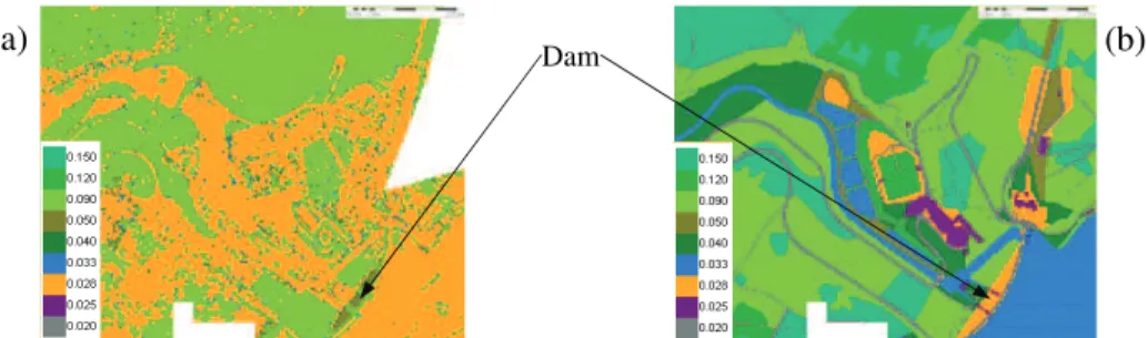
Variant 1: ditribution according to the difference between extreme laser echoes
The laser altimetry provides basically two values at each point, respectively named “first” and “second” echoes. The former generally corresponds to the elevation of the top of vegetation, while the later is the ground level. The idea is here to compute the local difference between these two echoes to infer a distribution of the friction coefficient between 0.03 and 0.11 s/m1/3, in accordance with the results of RESCDAM (2000).
Variant 2: interpretation of landuse maps
Besides, generally available landuse maps are worth being exploited. This type of maps provides the distribution of landuse, which can be from coarse (distinction of a few types of surfaces) to precise (distinction of different species in each category, so be it different types of trees, roads, buildings…). They result in a spatial distribution of the roughness coefficient, based on a mapping assumed between 10 different landuse categories considered as relevant in this case and classical values of Manning coefficients.
(a) Dam (b)
Figure 3: Distribution of the roughness coefficient in the vicinity of the dam, using –(a) difference of echoes –(b) landuse data.
RESULTS AND DISCUSSION
The 2D unsteady flow simulations provide large sets of results which are generally presented by means of hazard maps, such as time of arrival of the wave, maximal water levels, maximal unit discharges or velocity.
The hazard map representing the time of arrival of the front reveals that this result is monotonously increasing for an increasing friction coefficient. The landuse distribution deduced from the LiDAR echoes leads to times of arrival of the front almost systematically similar to than those obtained with a uniform Manning coefficient of 0.06 s/m1/3. This is consistent with the average value computed on the inundation extent. The curve corresponding to the landuse distribution lies generally in-between those related to 0.05 s/m1/3 and 0.06 s/m1/3, but more changes in the relative position are found due to the stronger local variations of the friction coefficient.
Maximum water levels reached in the main channel have also been extracted from the corresponding hazard map and are shown in Figure 4. These results are more complex to interpret since even when focusing on uniform distributions, comparison of the results shows non monotoneous evolutions with the friction coefficient. Two
conflicting trends are indeed competing. On one hand, the higher the friction coefficient, the more head is needed for the front to propagate and thus the more water is stored in upstream of obstacle or narrowings of the valley, leading to higher maximal water depths. On the other hand, this storage causes a damping of the hydrograph, which may in turn lead to lower maximum water depths further downstream.
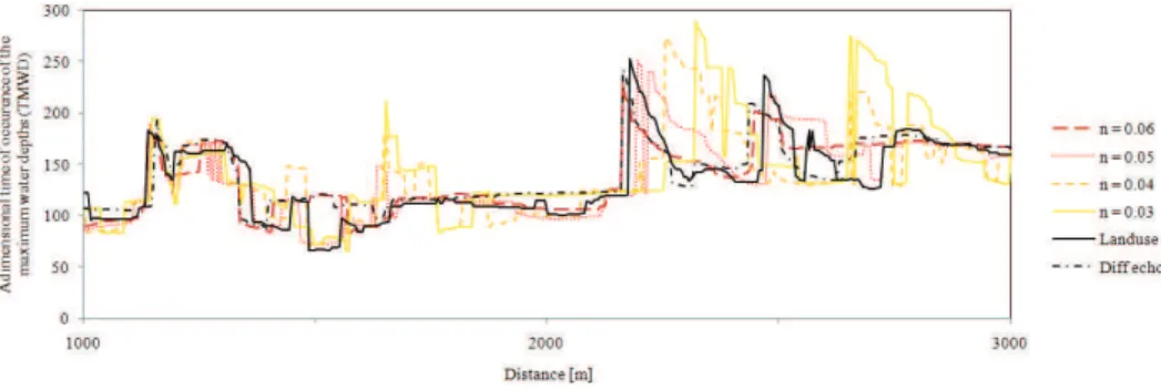
In addition, Figure 5 reveals that the time of occurrence of the maximum water depth doesn’t simply increase monotonously from upstream towards downstream. They demonstrate that maximum water depths may be reached not only as a result of the propagation of the main wave, but they may also be induced by complementary effects such as wave reflection on obstacles (e.g. at the entry of the town) or release of water temporarily stored in lateral valleys.
It is from practical interest to note that the maximum water depths show a very different sensitivity with respect to the friction coefficient depending on the location in the downstream valley. Therefore, applying a safety factor of, for instance an increase or decrease by 10-15% of the computed time of arrival of the front or maximal water depth as prescribed in French guidelines, may be correct for the time of arrival of the front but is not a suitable option for the maximum water depths. The actual envelope of the results should preferably be computed based on a wide range of friction coefficients.
Sudden narrowing City entrance
Valley enlargement Lateral valley
Figure 4: Maximum water depths (MWD) in the main channel downstream of the dam, expressed as a percentage of the local MWD corresponding to n = 0.03.
Figure 5: Time of occurrence of the maximum water depths (TMWD), expressed as TMWD+t h0 g where h0 = initial depth in thereservoir.
CONCLUSIONS
Historically, the first simulations of dam breaks had to consider the macro-roughness of buildings through the roughness coefficient, due to coarse DEM representing the ground topography. Then, increased computational capacities fed by new data collection lead to a consideration of the macro-roughness directly through the topography itself with a more comprehensive use of constant friction coefficient that were typical only of the surface roughness.
In this paper, a new step is suggested consisting in suitable data exploitation considering either landuse data or the difference between LiDAR echoes. These enhancements were substantiaded by laboratory tests performed with a focus, among others, on vegetation and land cover.
These preliminary results reveal the interest of going further in the spatial description of morphology established from comparative analysis of landuse and airborne laser altimetry.
AKNOWLEDGMENTS
The authors gratefully acknowledge the “Service Public de Wallonie” for funding the research project and for providing data.
REFERENCES
Alcrudo, F., Garcia-Navarro, P., and Saviron, J.-M. (1992). "Flux difference splitting for 1D open channel ow equations." Int. J. Numer. Methods Fluids, 14(9), 1009-1018.
Archambeau, P. (2006). "Contribution à la modélisation de la genèse et de la propagation des crues et inondations," University of Liege.
Bellos, C. V., and Sakkas, J. G. (1987). "1-D Dam-Break Floow-Wave Propagation on Dry Bed." J. Hydraul. Eng.-ASCE, 113(12), 1510-1524.
Dewals, B. (2006). "Une approche unifiée pour la modélisation d'écoulements à surface libre, de leur effet érosif sur une structure et de leur interaction avec divers constituants," University of Liege, PhD thesis.
Dewals, B., Erpicum, S., Archambeau, P., Detrembleur, S., and Pirotton, M. (2006a). "Theoretical and numerical analysis of the hydrodynamic waves induced by dam breaks and their interaction with structures located downstream." 7th
National Congress on theoretical and applied Mechanics, Mons, Belgium. Dewals, B. J., Erpicum, S., Archambeau, P., Detrembleur, S., and Pirotton, M.
(2006b). "Depth-integrated flow modelling taking into account bottom curvature." J. Hydraul. Res., 44(6), 787-795.
Dewals, B. J., Erpicum, S., Archambeau, P., Detrembleur, S., and Pirotton, M. (2006c). "Numerical tools for dam break risk assessment: validation and application to a large complex of dams." Improvements in reservoir construction, operation and maintenance, H. Hewlett, ed., Thomas Telford, London, 272-282.
Dewals, B. J., Erpicum, S., Archambeau, P., Detrembleur, S., and Pirotton, M. (2008). "Hétérogénéité des échelles spatio-temporelles d'écoulements hydrosédimentaires et modélisation numérique." Houille Blanche-Rev. Int.(5), 109-114.
Erpicum, S. (2006). "Optimisation objective de paramètres en écoulements turbulents à surface libre sur maillage multibloc," University of Liege, PhD thesis. Erpicum, S., Archambeau, P., Dewals, B., Detrembleur, S., and Pirotton, M. (2004).
"Computation of the Malpasset dam break with a 2D conservative flow solver on a multiblock structured grid." Proc. 6th Int. Conf. of Hydroinformatics, Singapore.
Erpicum, S., Dewals, B. J., Archambeau, P., and Pirotton, M. (2009a). "Dam-break flow computation based on an efficient flux-vector splitting." J. Comput.
Appl. Math., accepted.
Erpicum, S., Mao, Y., Pirotton, M., and Lejeune, A. (2006). "Process-oriented pollutant transport modelling in rivers networks - Application in the Xizhijiang River in China." 3rd Int. Symp. on integrated water ressources
management, Ruhr University, Bochum, Germany.
Erpicum, S., Meile, T., Dewals, B. J., Pirotton, M., and Schleiss, A. J. (2009b). "2D numerical flow modeling in a macro-rough channel." Int. J. Numer. Methods
Fluids, published online: 13 Feb 2009.
Fennema, R. J., and Chaudhry, H. (1990). "Explicit Methods for 2-D Transient Free Surface Flows." J. Hydraul. Eng.-ASCE, 116(8), 1013-1034.
Fread, D. L. (1984). "DAMBRK: The NWS Dam Break Flood Forecasting Model." National Weather Service (NWS) Report, Silver Spring, MA, USA.
Garcia-Navarro, P., Fras, A., and Villanueva, I. (1999). "Dam-break flow simulation: some results for one-dimensional models of real cases." J. Hydrol., 216, 227-247.
Glaister, P. (1988). "Approximate Riemann Solutions of the Shallow Water Equations." J. Hydraul. Res., 26(3), 293-300.
Kerger, F., Archambeau, P., Erpicum, S., Dewals, B. J., and Pirotton, M. (2009). "Simulation numérique des écoulements mixtes hautement transitoires dans les conduites d'évacuation des eaux." Houille Blanche-Rev. Int., accepted. Khuat Duy, B., Archambeau, P., Erpicum, S., Dewals, B. J., and Pirotton, M. (2009).
"Modélisation hydrologique à grande échelle des zones imperméables égouttées." Houille Blanche-Rev. Int., accepted.
Pirotton, M. (1994). "Modélisation des discontinuités en écoulement instationnaire à surface libre. Du ruissellement hydrologique en fine lame à la propagation d'ondes consécutives aux ruptures de barrages," Thèse de doctorat, Université de Liège, Liège.
RESCDAM. (2000). "The use of physical models in dam-break flood analysis - Final report." Helsinki University of Technology.