G. Grosjean1, G. Lagubeau1,2, A. Darras1, M. Hubert1, G. Lumay1 & N. Vandewalle1
Physics governing the locomotion of microorganisms and other microsystems is dominated by viscous damping. An effective swimming strategy involves the non-reciprocal and periodic deformations of the considered body. Here, we show that a magnetocapillary-driven self-assembly, composed of three soft ferromagnetic beads, is able to swim along a liquid-air interface when powered by an external magnetic field. More importantly, we demonstrate that trajectories can be fully controlled, opening ways to explore low Reynolds number swimming. This magnetocapillary system spontaneously forms by self-assembly, allowing miniaturization and other possible applications such as cargo transport or solvent flows.
A Reynolds number much smaller than unity indicates that viscous forces dominate over inertial forces in a given flow. This is usually the case at the microscopic scale, which strongly impacts locomotion mech-anisms of both biological and artificial microswimmers. Indeed, to swim by changing its shape, a micro-scopic body must break time-reversal symmetry1–3. Methods for producing artificial microswimmers are
being actively researched4–8. One major unanswered problem is the control of swimming direction. A
fine control of swimming trajectories would be required for most practical applications, such as manip-ulation and transport of small elements9 or micro-scale fluid flow generation10. Furthermore, complex
fabrication processes could limit potential micro-scale applications. Self-assembled systems present a clear advantage in this regard, as they require no direct manipulation of micro-components11–13. Floating
soft-ferromagnetic particles have been shown to produce self-assembled structures when exposed to magnetic fields14. Oscillating fields can deform these assemblies in a way that produces low Reynolds
locomotion, although by which mechanism remains obscure15. In the present paper, we propose an
expla-nation for the breaking of time-reversal symmetry in magnetocapillary swimmers, as well as demonstrate how swimming speed and direction can be finely controlled in order to produce the desired trajectories.
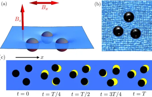
Three soft ferromagnetic spheres of size D are gently placed along a water-air interface, at the center of a triaxial Helmholtz system. The weight of the particles creates menisci that induce an attractive cap-illary interaction between neighboring beads16, as shown in Fig. 1(a,b). Soft ferromagnetic particles are
used, in which magnetic dipoles are induced along the direction of B with negligible hysteretic behavior.
A magnetization cycle of the beads can be found at17. As a consequence, the breaking of time reversibility
in our system does no come from magnetic hysteresis, as was proposed in recent studies based on two-particle systems18. When the particles are in presence of a magnetic field =B B e +B e
x x z z,
dipole-dipole interaction competes with capillary attraction. A vertical magnetic field (Bx = 0) leads to
the formation of a regular triangle, which size can be tuned by Bz14,19, as shown in the supplementary
video 1. In the following, the vertical field is kept constant at Bz = 30 G such that the bead center-to-center
distance is close to two bead diameters 2D. When a constant horizontal field is added, symmetry break-ing occurs in the system which then forms an isosceles. An oscillatbreak-ing horizontal field Bx=βx sin 2( πft) thus periodically deforms the triangular structure. Amplitudes βx larger than Bz/2 cannot be reached
because the system collapses, leading to hysteretic contacts19 between the beads.
In Fig. 1(c), one observes that small deformations of the triangle are accompanied by large rota-tional motions of the whole structure. Those repeated deformations/rotations come from the competition between magnetic, capillary and hydrodynamic interactions15. A significant motion of the bead triplet 1GRASP, Institute of Physics B5a, University of Liège, B4000 Liège, Belgium. 2Departemento de Física, Universidad de Santiago de Chile, Santiago de Chile. Correspondence and requests for materials should be addressed to N.V. (email: [email protected])
Received: 16 February 2015 Accepted: 07 October 2015 Published: 05 November 2015
www.nature.com/scientificreports/
can be seen in Fig. 1 or in the supplementary video 2. Swimming has been found for frequencies f in between 0.1 Hz and 3 Hz. In the following paper, a frequency of 0.5 Hz has been chosen as a compro-mise between low Reynolds number and practical constraints linked to experiment running time. The relevant Reynolds number in the system is that of the individual particles, which in this case has typical values around Re ≈ 10−1. It is possible, however, to further lower frequency f and/or field amplitude β
x
in order to emphasize that low Reynolds locomotion takes place, reaching typical values in the range Re = [10−3, 10−2]. Another relevant dimensionless number in the system is the Stokes number, which
can be defined as the ratio between the inertia of a particle and viscous forces. In that case, it can be shown that St ≈ Reρp/ρf where ρp and ρf represent the densities of the particle and the fluid, respectively.
In the present situation, steel beads immersed in water give a ratio ρp/ρf = 7.81. Therefore, although St
can approach unity in some cases, swimming has been observed down to St ≈ 10−2 with little qualitative
difference. This suggests that neither fluid inertia nor bead inertia are the main ingredient required to explain the breaking of symmetry in this case20. One should notice that earlier studies on surface
swim-mers using magnetic particles relied on surface waves6,7. In these experiments, locomotion at Re ≈ 100
appears due to waves generated by oscillating particle chains. This differs from our system, in which chain formation is not allowed and frequencies are much lower. As a consequence, vertical motion of the interface is negligible and capillary wavelength is much larger than the system, as was determined in previous work15.
Results
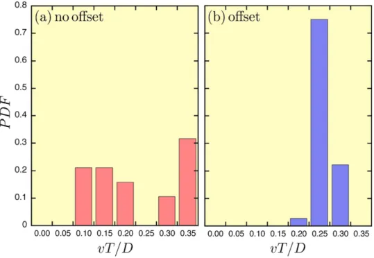
Figure 2 presents the Probability Distribution Function (PDF) of the normalized speeds for several swim-mers using the same set of parameters : (a) without any offset and (b) with a small offset Bx0 = 0.75 G.
The swimming speed is found to be broadly distributed in the first case while it exhibits a narrow peak in the second case. In fact, various pulsation modes can be observed when the horizontal field oscillates, particularly with different initial conditions. The offset Bx0 helps the triplet to select a unique oscillation
mode. The speed is then narrowly distributed, with only small fluctuations due to experimental varia-tions, such as in bead properties, wetting conditions and small flows in the bath. The horizontal field becomes Bx = [Bx0 + βxsin(2πft)]. One should remark that the offset enhances the deformation of the
triangle but is kept as low as possible here in order to avoid the collapse of the structure.
Figure 3(a) shows the resulting speed v of the assembly normalized by the bead diameter D per forcing period T = 1/f, as a function of the amplitude of the field oscillations βx. For small oscillations Figure 1. Self-assembled magnetocapillary swimmer. (a) Sketch of the magnetocapillary system. Soft
ferromagnetic particles are self-assembling at the water-air interface in a Petri dish. A vertical and constant magnetic field Bz is applied through the system. An oscillating horizontal field Bx excites the motion of the self-assembled structure. (b) A top view of the interface emphasizes the self-assembly of D = 500μm beads in a vertical field: capillary attraction is counterbalanced by dipole-dipole repulsion. The deformation of the liquid-air interface is evidenced by placing an array of pixels underneath the Petri dish. (c) Five snapshots of the beads over one period T of the forcing oscillation. The traces of the initial positions are drawn in yellow for emphasizing the motion of the structure. One should notice the rotational oscillation of the structure during the period.
(regime I), no significant motion is observed. When the amplitude βx of the field oscillations becomes
much larger than the offset Bx0 (regime II), the speed increases and saturates at high field values. The
dimensionless speed reaches about 0.3 D/T, which can be considered an efficient locomotion speed in the Stokes regime21,23. Amplitudes larger than β
x = 15G cannot be used because the system collapses,
leading to contacts between the beads. Close to collapse (regime III), speed exhibits large fluctuations, as seen in Fig. 3(a). It has proven hard to control the speed and the pulsation mode in that regime. We also noticed that large offset values reduce the efficient locomotion (regime II) into a sharp range of βx values. Figure 2. Selection of swimming modes. Probability Distribution Function (PDF) of normalized speeds
obtained in similar experimental conditions: βx = 7.5 G and f = 0.5 Hz, but (a) without an offset, (b) with a constant offset Bx0 = 0.75 G. The plots are obtained from 55 independent realizations.
Figure 3. Swimming speeds. (a) Average speed of the self-assembled system as a function of the amplitude
of oscillations, when the offset is Bx0 = 0.75 G and f = 0.5 Hz. The velocity is seen to increase and saturates around 0.3 D/T. The curve is a guide for the eye. (b) The maximum standard deviation δ of the angles from the regular triangle as a function of the amplitude βx. The curve is a guide for the eye. Please note the large differences obtained near the collapse (βx ≈ 15 G). Three regimes (I, II and III) are indicated and are discussed in the main text.
www.nature.com/scientificreports/
In order to quantify the triplet deformations, we computed the standard deviation δ of the internal angle departures (αi − 60) from the regular triangle (in degrees), i.e.
∑
δ= (α − ) . ( ) = 1 3i 1 i 60 1 3 2The maximum value of this parameter over a period max {δ} is shown in Fig. 3(b) as a function of βx.
When βx increases from zero, max {δ} presents a jump similar to v above Bx0 before saturating to around
2 degrees (regime II). The speed v and deformation δ are therefore correlated. It should be stressed that the deformation is relatively weak such that the locomotion should be linked to some additional motion of the beads such as the structure rotation. However, for higher amplitudes close to the collapse (regime III), the triangle is highly stretched providing much higher values of δ where the speed fluctuates.
The major ingredient triggering the locomotion is the field amplitude βx. Once the triangle
pulsa-tion is selected, the oscillapulsa-tion mode remains unchanged and the swimmer trajectory is a straight line. Although different from the x-axis, the swimming direction is in fact correlated to the oscillating field direction. Indeed, Fig. 4 presents three independent trajectories of swimmers which are prepared by adjusting slowly the horizontal magnetic field direction in the x − y plane in order to induce U-turn, corner and loops, proving that the remote control can be fully exploited. The paths form the letters of “ULg”, being the logo of our University. The video of the U-turn is given in the supplementary materials. Slowly adjusting the horizontal field orientation offers therefore a convenient way to control the path of a microswimmer.
Discussion
Two main mechanisms can provide the breaking of time reversibility necessary for low Reynolds loco-motion. Symmetry breaking can either occur in the sequence of shapes adopted by the swimmer1 or in
the viscous drag felt by the swimmer22. Here, comparing typical strength of magnetic force ≈ µ
π Fm 340mr2
4
and hydrodynamic interaction ≈F πη
h 6 R Ur
2
, where m is the magnetic moment of a bead, R its radius, U its speed and r is the center-to-center distance, yields a ratio ≈ 5 10FFm 2
h . The shape of the swimmer is
thus driven by magnetic dipole-dipole interactions in our case. Note that hydrodynamics must be taken into account to fully explain the locomotion, as no swimming is possible in the absence of a flow. However, to study the shapes adopted by the swimmer and the breaking of time reversibility, hydrody-namics do not play any significant role compared to magnetism.
A magnetocapillary model, similar to23 and based on the magnetic and capillary interactions only,
allows us to capture the possible beads configurations when both vertical and horizontal magnetic fields are applied. Moreover, it provides clues for the origin of the non-reciprocal motion behind low Reynolds locomotion, as seen below. For convenience, distances rij between beads i and j are adimensionalized by
the capillary length, being the characteristic length of capillary interactions λ= γ ρ/ g ≈ .2 7mm16.
Considering only quasi-static situations, i.e. excluding hydrodynamic interactions, the dimensionless bead-bead potential is given by
Figure 4. Full control of swimming trajectories. The remote control of a microswimmer, by adjusting the
horizontal field orientation e, allows us to follow various paths such as U-turn, corner and loops. Laid next to one another, the three letters of “ULg” are then obtained. Bead centers are tracked for drawing the triangles at each period, emphasizing the orientation of the structure. The colors indicate the time evolution of each trajectory from dark to red.
(
)
= − ( ) + + − . ( ) u K r r r r e r Mc Mc 1 3 2 ij ij ij ij ij x ij 0 3z x 3 2 5where Mcz and Mcx are magnetocapillary numbers23 measuring the competition between magnetic and
capillary interactions. The Bessel function K0(r) is assumed to capture the attractive capillary
interac-tion16. Each magnetocapillary number is proportional to dipole-dipole interactions. One can fix the
num-ber Mcz in order to obtain an equilibrium distance rij = 2D/λ = 0.3 when the horizontal field is zero
(Mcx = 0, Mcz ≈ 0.01). This distance corresponds to what we observe in our experiments. The parameter
/
Mc Mcx z becomes then the only relevant parameter in the problem, reducing to the ratio Bx/Bz. In
order to study the equilibrium configurations, we start from a regular triangle with edge length r = 0.3, the horizontal field is slightly modified and the new equilibrium situation is found by simulated anneal-ing searchanneal-ing for the local minimum of u = u12 + u23 + u31, by producing tiny random moves for bead
positions. The results of these simulations are discussed below.
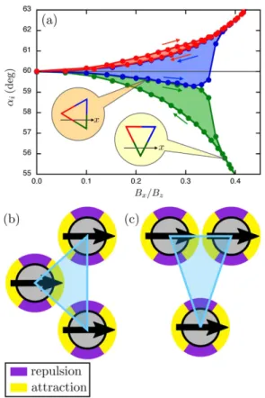
Figure 5(a) presents the evolution of the internal angles αi of the triplet at equilibrium and for
different values of an increasing then decreasing horizontal field, i.e. when the ratio Bx/Bz follows a
quasi-static cycle. Arrows indicate how the structure evolves. The collapse of the structure takes place around Bx/Bz ≈ 1/2, as expected. In presence of a horizontal field, the triangle is roughly isosceles during
the whole cycle since two angles are always close together. At low and increasing field strengths, one angle is larger than 60° and the other angles have similar values below 60°. For the lack of a proper term, we labelled this first type of isosceles “platy-isosceles”. It is characterized by internal angles
α( ) = δ δ δ + , − , − ( ) 60 2 60 2 60 2 3 i
Figure 5. Model for non-reciprocal motion. (a) Internal angles given by the model as a function of the
increasing or decreasing horizontal magnetic interaction (see arrows). Angles αi are colored after being sorted from the smallest to the largest. Two triangles are illustrated using the same color code in order to evidence the orientation of the structure at two specific situations: and ∇ states. (b) Sketch of the platy-isosceles () configuration. Arrows indicate the horizontal components of the dipoles. Colors indicate whether a pair of dipoles attract or repel compared to zero horizontal field, which depends on their relative orientation. (c) Sketch of the lepto-isosceles (∇ ) configuration.
www.nature.com/scientificreports/
and occurs when one edge is perpendicular to the field axis, as sketched in the inset of Fig. 5(a). By symmetry, two configurations can be obtained: left () and right (). Above some field strength, the system drastically changes since two angles have similar large values while the later is much smaller than 60°. One has a second type, labelled “lepto-isosceles”, given by
α(∇) = δ δ δ + , + , − ( ) 60 2 60 2 60 2 4 i
which is encountered when one side is parallel to the field. Two equivalent configurations are found: up (Δ ) and down (∇ ). In fact, this bifurcation between platy to lepto-isosceles, e.g. → ∇ , is accompanied by a rotation of 30° of the entire structure, as sketched in the Fig. 5(a). The system remains trapped in this last configuration till returning to a regular triangle at zero field. Figure 5(b,c) represents three dipoles in both platy and lepto-isosceles configurations. As a reminder, horizontal components of the dipole-dipole interaction can either generate an attraction or a repulsion, depending on the relative ori-entation of the dipoles. This is described by the sign of the last term in equation 2 and represented by a color code in Fig. 5(b,c). These attractions/repulsions determine the shape of the triangle. Because all dipole pairs are not aligned in a triangular configuration, the system is energetically frustrated.
Such a switching behavior between two states is observed periodically in experiments. Indeed, Fig. 6(a) presents the evolution of the angles αi during three successive periods using the same color
code: largest angle in red, lowest angle in green. During each period, the main qualitative characteristics predicted by the model are recovered: short successive periods during which both types of isosceles are seen. It should be noted that the model does not predict which configuration is chosen when the field goes back to zero. At zero field, small residual magnetization becomes relevant and might explain why the same configuration is always chosen, such that deformation is periodical. This could also explain the influence of initial conditions on swimming velocities that was observed in Fig. 2(a). One should also remark that the experimental curves are much more complex than numerical ones due to the presence of hydrodynamic interactions and additional effects, such as a slow rotation of the beads due to tiny residual magnetization. Because of the presence of these additional effects, the angles exhibit periodic jumps from one isosceles type to the other one. Figure 6(b) presents the evolution of the orientation of the entire structure during the same three periods. The angle θ is seen to oscillate over one period, as expected. Figure 6(c) illustrates the non-reciprocity of the shape succession necessary to propulsion. It
Figure 6. Non-reciprocal motion in the experiment. (a) Three periods T of the angles αi with the same color code as in Fig. 5(a), using our experimental data. One observes that the blue curve oscillates between the red and green ones in each period. The system switches periodically between and ∇ isosceles. (b) The angle θ of the whole structure during three periods. Oscillations are seen evidencing the successive switches. (c) This sketch shows the isosceles states as a function of θ forming a loop at each cycle, i.e. a non-reciprocal motion.
Methods
Hereinafter, we present methods and experimental setup. A large Petri dish is filled with water. The liquid/air interface is placed at the center of a triaxial Helmholtz system that compensates the Earth magnetic field, and that is able to produce a uniform field in any direction. When a current i is injected in such coils, a uniform and vertical magnetic field Bz is obtained in the Petri dish. Magnetic fields up to
30 G have been considered. Oscillations of the horizontal field Bx are provided by a function generator
and an amplifier. Chrome steel particles (selected alloy AISI 52100, ρs = 7830 kg/m3) are soft
ferromag-netic beads, and they do not exhibit any hysteretic behavior in the range of field values used herein. As a result, particles retain a negligible residual magnetic moment once the field is removed. We have estimated this residual magnetization to be roughly 50 times lower than the induced magnetization due to the applied field. Prior to experiments, spheres are washed with isopropyl alcohol and thereafter dried in an oven. Different bead diameters have been studied but the results shown herein correspond to D = 500μm. At this scale, partial wetting ensures the floatation of the spheres. A CCD camera records images from above. Image analysis provides the position of each bead as a function of time.
References
1. Purcell, E. M. Life at low Reynolds number. Am. J. Phys. 45, 3–11 (1977). 2. Lauga, E. Life around the scallop theorem review. Soft Matter 7, 3060–3065 (2011).
3. Lauga, E. & Powers, T. R. The hydrodynamics of swimming microorganisms. Rep. Prog. Phys. 72, 096601 (2009). 4. Dreyfus, R. et al. Microscopic artificial swimmers. Nature 436, 862–865 (2005).
5. Snezhko, A. & Aranson, I. S. Magnetic manipulation of self-assembled colloidal asters. Nature Mat. 10, 698–703 (2011). 6. Snezhko, A., Belkin, M., Aranson, I. S. & Kwok, W.-K. Self-Assembled Magnetic Surface Swimmers. Phys. Rev. Lett. 102, 118103
(2009).
7. Piet, D. L., Straube, A. V., Snezhko A. & Aranson, I. S. Viscosity Control of the Dynamic Self-Assembly in Ferromagnetic Suspensions. Phys. Rev. Lett. 110, 198001 (2013).
8. Williams, B. J., Anand, S. V., Rajagopalan, J. & Saif, M. T. A. A self-propelled biohybrid swimmer at low Reynolds number. Nature
Comm. 5, 3081 (2014).
9. Tottori, S. et al. Magnetic Helical Micromachines: Fabrication, Controlled Swimming, and Cargo Transport. Adv. Mater. 24, 811–816 (2012).
10. Darnton, N., Turner, L., Breuer, K. & Berg, H. C. Moving fluid with bacterial carpets. Biophys. J. 86, 1863–1870 (2004). 11. Whitesides, G. M. & Grzybowski, B. Self-assembly at all scales. Science 295, 2418–2421 (2002).
12. Pelesko, J. A. Self-Assembly (Chapmann & Hall, Boca Raton, 2007).
13. Davies, G. B., Krüger, T., Coveney, P. V., Harting, J. & Bresme, F. Assembling Ellipsoidal Particles at Fluid Interfaces Using Switchable Dipolar Capillary Interactions. Adv. Mater. 26, 6715–6719 (2014).
14. Vandewalle, N., Obara, N. & Lumay, G. Mesoscale structures from magnetocapillary self-assembly. Eur. Phys. J. E 36, 127 (2013). 15. Lumay, G., Obara, N., Weyer, F. & Vandewalle, N. Self-assembled magnetocapillary swimmers. Soft Matter 9, 2420–2425 (2013). 16. Vella, D. & Mahadevan, L. The ‘Cheerios effect’. Am. J. Phys. 73, 817–825 (2005).
17. Lumay, G. & Vandewalle, N. Tunable random packings. New J. Phys. 9, 406 (2007).
18. Ogrin, F. Y., Petrov, P. G. & Winlove, C. P. Ferromagnetic microswimmers. Phys. Rev. Lett. 100, 218102 (2008).
19. Vandewalle, N. et al. Symmetry breaking in a few body system with magneto-capillary interactions. Phys. Rev. E 85, 041402 (2012).
20. Lagubeau, G. et al. Statics and dynamics of magnetocapillary bonds. arXiv:1508.01885 preprint (2015).
21. Ledesma-Aguilar, R., Lowen, H. & Yeomans, J. M. A circle swimmer at low Reynolds number. Eur. Phys. J. E 35, 70 (2012). 22. Tierno, P., Golestanian, R., Pagonabarraga, I. & Sagus, F. Controlled swimming in confined fluids of magnetically actuated
colloidal rotors. Phys. Rev. Lett. 101, 218304 (2008).
23. Chinomona, R., Lajeunesse, J., Mitchell, W. H., Yao, Y. & Spagnolie, S. E. Stability and dynamics of magnetocapillary interactions. preprint arXiv:1410.0429 (2014)
24. Olla, P. Pros and cons of swimming in a noisy environment. Phys. Rev. E 89, 032136 (2014).
25. Najafi, A. & Golestanian, R. Simple swimmer at low Reynolds number: Three linked spheres. Phys. Rev. E 69, 062901 (2004).
Acknowledgements
This work was financially supported by the FNRS (Grant PDR T.0043.14) and by the University of Liège (Grant FSRC 11/36). GG thanks FRIA for financial support. GLa was financed by the University of Liège and the European Union through MSCA-COFUND-BeIPD project.
www.nature.com/scientificreports/
Author Contributions
G.G., G.L. and A.D. collected and analyzed experimental data. Physical interpretations were provided by M.H., G.L. and N.V. This manuscript was written by N.V.
Additional Information
Supplementary information accompanies this paper at http://www.nature.com/srep Competing financial interests: The authors declare no competing financial interests.
How to cite this article: Grosjean, G. et al. Remote control of self-assembled microswimmers. Sci. Rep. 5, 16035; doi: 10.1038/srep16035 (2015).
This work is licensed under a Creative Commons Attribution 4.0 International License. The images or other third party material in this article are included in the article’s Creative Com-mons license, unless indicated otherwise in the credit line; if the material is not included under the Creative Commons license, users will need to obtain permission from the license holder to reproduce the material. To view a copy of this license, visit http://creativecommons.org/licenses/by/4.0/