Assessing the Proximity of Time Evolutions through Dynamic Time Warping
Davide Fabozzi1 and Thierry Van Cutsem2
1D. Fabozzi ([email protected] ) : Department of Electrical Engineering and Computer Science
(Monte-fiore Institute), University of Li`ege, Sart Tilman B37, B-4000 Li`ege, Belgium
2T. Van Cutsem ([email protected]) : Fund for Scientific Research (FNRS) and Department of Electrical
Engineering and Computer Science of the University of Li`ege, B37, B-4000 Li`ege, Belgium
Abstract. Comparing time-series is a frequent task in many scientific fields. In power systems, in particular, it may be of interest to compare the outputs of a simplified and a detailed model, or to validate the output of a model with respect to a measured time response. The classical Euclidean distance, involving pairs of points of the two data series aligned in time, is not suited to the practical time evolutions met in power systems, which often involve variable time delays and jumps at discrete times. In this paper, an alternative measure of proximity, stemming from other scientific fields, is proposed for power system applications. It consists in warping the time axis to guarantee the best match between the two time-series, i.e. it maps points on two curves that are not aligned in time so as to minimize the sum of squared differences of their ordinates. Modifications and adaptations of the classical algorithm to better fit power system problems are discussed. The method is illustrated through three representative curve comparison problems. A multi-dimensional extension allowing system-wide measures of similarity is also proposed.
Keywords. Time-series, curve matching, proximity measure, Euclidean distance, dynamic time warping, dynamic programming, system-wide validation.
1
Introduction
Comparison of time-series occurs in numerous scientific disciplines. The problem is to assess how close a dynamic evolution characterized by a time-series q = [q1, q2, . . . , qn] is to a reference characterized by a time-series
r = [r1, r2, . . . , rn]. The former is referred to as the query and the latter as the reference time-series.
In the power system literature, the accuracy of query with respect to reference is often depicted by qualitative, and admittedly subjective, evaluation terms such as “we see a good overall match between q1and r”, “q2and r
have nearly the same degree of accuracy” or “q3is almost undistinguishable from r”, etc. The objective of this
paper is to promote the use of a less subjective measure of proximity.
Assuming that both time-series span the same time interval and are uniformly sampled at the same n time instants, a simple measure of proximity is the Euclidean distance between q and r defined as:
E(q, r) = v u u t∑n i=1 (qi− ri)2 (1)
In many cases, this distance is not an effective measure of similarity. For instance, for the two time-series depicted in Fig. 1, a mere visual inspection shows that the two curves are merely shifted in time, which is not significant in usual power system applications. While both curves should be considered quite close to each other, the Euclidean distance does not recognize the pattern similarity and takes on a large value.
t
Figure 1: Two shifted damped sinusoids
More complex validation metrics that can overcome this problem are used in the field of computational me-chanics: the metrics reviewed in [1] give a measure in terms of magnitude and phase differences. This would correctly identify the similarity between the curves in Fig. 1. However, the measure of magnitude and phase differences correctly identifies a time shift only if (i) the latter is constant throughout the whole time interval, and (ii) the initial and final values coincide. Unfortunately, both assumptions are seldom valid for power system time responses, where: (i) discrete events can take place at slightly different time instants, (ii) the time-shift may vary in time, and (iii) the system may settle to a different state or even collapse after a disturbance. A typical voltage
collapse case, where neither Euclidean distance nor magnitude and phase difference measures would perform well, will be assessed later on in Section. 5.1. Thus, the above quoted measures of proximity are not suited to compare time-series involving events and phenomena typical of power system dynamics.
An interesting alternative is Dynamic Time Warping (DTW), an algorithm originally developed some decades ago for speech recognition [2, 3] and now used in various fields such as medicine [4], data mining [5], signature verification [6], and others.
DTW warps the time axis to guarantee the best match between both time-series. More precisely, it maps the points of both curves so that the sum of their squared ordinate differences is minimum, under some constraints. This is equivalent to determining the deformation of the time axes which brings the two time-series as close as possible in the Euclidean-norm sense. The minimization is performed with the help of an efficient dynamic programming algorithm.
The so obtained, more rigorous measure of proximity has several potential applications in power system dy-namics. For instance, in the context of simplified simulations, it can be used to evaluate the relative accuracy of one simulation with respect to another. In the context of model validation, DTW yields an objective measure of proximity between a simulated response and a measured reference. It can be also used to classify power quality events [7] or to detect instability modes [8].
The paper is organized as follows. Section 2 describes the principle and determination of the DTW distance. In Section 3 some algorithmic improvements and adaptations to typical power system evolutions are proposed, while additional aspects are discussed in Section 4. Examples of application to solver and model validation are provided in Section 5. The paper ends with the Conclusion in Section 6.
2
Principle and determination of DTW distance
2.1
Definition of DTW distance
For the sake of simplicity, the query and reference time-series are supposed to cover the same time span, have the same number n of points, and be uniformly sampled. Note that the method can be adapted to the case of non-uniform samplings or different time spans. Alternatively, the time-series could be cropped and uniformly re-sampled before applying the method. Further discussions on sampling can be found in Section 4.
Let us define the squared distance between one point of q and one point of r as :
ℓ(i,j)= (qi− rj)2 i, j = 1, . . . , n (2)
The Euclidean distance in between the two time-series is given by:
E(q, r) = v u u t∑n i=1 ℓ(i,i) (3)
Relaxing the constraint that the associated points of q and r relate to the same time instants, we define a warping path as an N -dimensional array of pairs
w = [w1w2. . . wN] = [(i1, j1) (i2, j2) . . . (iN, jN)] (4)
where the first element of each pair is an index referring to a point of q and the second element to a point of r. In addition, a warping path obeys the following three constraints:
1. Boundary condition. The path starts at the initial point of both time-series, i.e. w1 = (1, 1), and ends at
the final point of both time-series, i.e. wN = (n, n). In Section 3 the requirement on the final point will be
somewhat relaxed to cope with evolutions not ending at the same time.
2. Continuity. Given wk = (i, j) and wk+1 = (i′, j′), the following inequalities hold true: i′ ≤ i + 1 and
j′ ≤ j + 1. Thus, the path does not “skip” any point of either time-series.
3. Monotonicity. Given wk = (i, j) and wk+1 = (i′, j′), the following inequalities hold true: i′ ≥ i and
j′ ≥ j and (i′− i) + (j′− j) ≥ 1. Thus, the path neither “goes back in time” nor “stalls”.
For a given warping path w, one can define the distance D between q and r along that path as:
D(q, r, w) = v u u t∑N k=1 ℓwk (5)
where ℓwkis the quantity defined by (2) for the pair (i, j) present in wk, the k-th component of w.
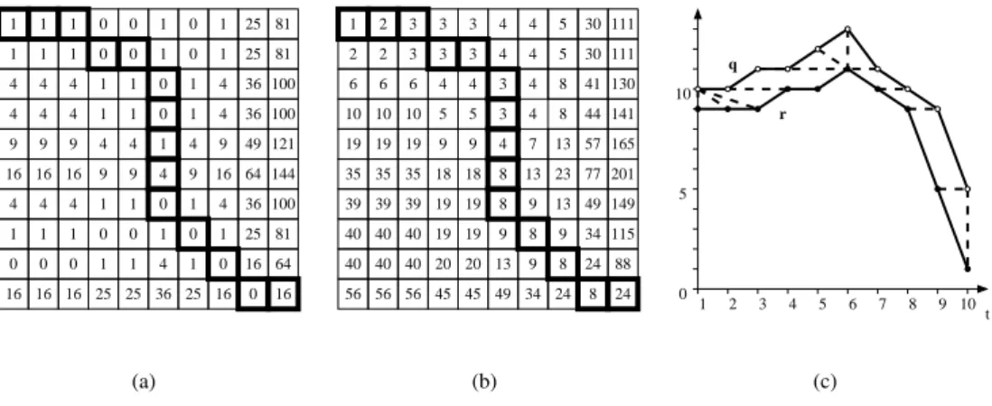
As an illustrative example, consider the two time evolutions shown in Fig. 2.c. A warping path is shown with dotted lines. This path can be better visualized on the local distance matrix L defined as follows:
(L)ij = ℓ(i,j) i, j = 1, . . . , n (6)
This matrix is shown in Fig. 2.a for the two time-series of concern. Starting from the upper left and ending in the lower right corners, the sequence of cells marked with heavy lines corresponds to the warping path shown
in Fig. 2.c. It is easily checked that this path obeys the continuity and monotonicity constraints. The latter allow passing from cell (i, j) to cell (i′, j′) through forward-forward (i′ = i + 1, j′ = j + 1), delay-forward (i′ = i, j′ = j + 1), and forward-delay (i′ = i + 1, j′ = j) moves. The corresponding distance D is the sum of the L matrix entries visited by the warping path.
t 0 16 25 36 25 25 16 16 16 r q 10 5 0 5 6 7 8 9 10 4 3 2 1 1 2 3 3 3 4 4 5 30 111 2 2 3 3 3 4 4 5 30 111 6 6 6 4 4 3 4 4 8 8 41 44 130 141 5 5 3 4 10 10 10 19 19 19 9 9 7 13 13 23 13 8 8 8 8 8 9 9 24 24 24 9 9 18 18 19 19 19 19 20 20 35 35 35 39 39 39 40 40 40 40 40 13 34 40 49 45 45 56 56 56 34 49 57 77 165 201 149 115 88 1 1 1 1 1 1 1 1 1 1 1 1 0 0 1 0 1 25 81 1 0 0 0 25 81 1 4 4 4 4 4 4 4 4 0 0 36 36 100 100 9 9 9 9 9 9 9 4 4 4 4 1 16 16 16 16 49 121 64 144 4 4 4 1 1 1 1 1 0 0 1 1 0 0 4 1 36 25 81 100 0 0 0 1 1 4 1 0 16 64 16 (a) (b) (c)
Figure 2: Classical DTW distance: local distance matrix L (a), accumulated distance matrix ∆ (b), query and reference plots with warped pairs (c)
To determine “how close” the time-series q and r are from each other, it is appropriate to consider the warping path which minimizes Dd(q, r, w), i.e. to determine the w⋆solution of:
min w D(q, r, w) = minw v u u t∑N k=1 ℓwk (7)
and use the corresponding distance D(q, r, w⋆) as the sought measure. The latter will be referred to as the DTW
distance.
Note that if one imposes N = n, the unique warping path is w = [(1, 1) (2, 2) . . . (n, n)], which lies along the diagonal of L, and D(q, r, w) coincides with the Euclidean distance E(q, r), which is also the square root of the trace of the L matrix.
Coming back to the example, the path emphasized in Fig. 2.a turns out to be the optimal warping path w⋆. One could check that no other association between the points of q and r (satisfying constraints 1 to 3) than the one shown with dotted lines in Fig. 2.c yields a smaller value of D(q, r, w). The corresponding DTW distance is:
D(q, r, w⋆) =√(3× 1) + (4 × 0) + 1 + 4 + (4 × 0) + 16 =√24 = 4.899
With reference to Fig. 2.c, it can be said that the optimal warping path defines the deformation of the time axes of q and r which brings the two time-series as close as possible to each other (in the Euclidean-norm sense) [4].
2.2
Determination of the optimum warping path
Finding the optimal warping path is a combinatorial optimization problem. In spite of the large search space, this problem can be solved with remarkable efficiency through Dynamic Programming (DP) [2, 3].
DP exploits the fact that each portion of the optimal warping path is itself an optimal warping path. More precisely the DP-based algorithm relies on the recursive formula:
D(q, r, w1⋆→k) = ℓwk+ D(q, r, w
⋆
1→k−1) (8)
with D(q, r, w⋆1→1) = ℓw1 = ℓ(1,1) (9)
where w⋆
1→kdenotes the first k components of w ⋆.
In practice, it is convenient to consider the accumulated distance matrix ∆ defined recursively as:
[∆]1j = j ∑ k=1 [L]1k j = 1, . . . , n (10) [∆]i1 = i ∑ k=1 [L]k1 i = 2, . . . , n (11) [∆]ij = [L]ij+ min{[∆]i−1,j−1, [∆]i,j−1, [∆]i−1,j} i, j = 2, . . . , n (12)
This matrix is built starting from the upper left corner. From (5, 7, 8, 9) is is easily shown that:
D(q, r, w⋆) = √
[∆]nn (13)
Coming back again to the example, Fig. 2.b shows the ∆ matrix computed by (10-12) from the L matrix shown in Fig. 2.a. Furthermore, the optimal warping path is identified by backtracking from the (n, n) entry of
∆, taking as predecessor of the (i, j) cell, the one among{(i − 1, j − 1), (i, j − 1), (i − 1, j)} with the lowest
value, and repeating the procedure until the (1, 1) cell is reached. It is easily checked that this simple procedure yields the path emphasized in Fig. 2.b.
Even if the computational cost of the DTW algorithm is not an issue for the off-line accuracy studies considered here, it may be of interest to reduce the computational burden of the DTW algorithm by using the technique proposed in [3]. The idea is to restrain the warping path from regions of the local distance matrix L which are
far from its diagonal. Thus, the warping path is searched in what has been eponymously called the Sakoe-Chiba band. In speech recognition some heuristics are used to choose the width of the band, which it would probably not make sense to transpose to power systems.
Instead, that width can be related to the largest acceptable time difference τmaxbetween any two associated
points (i.e. the largest acceptable time warping). When the query and reference curves span the same time interval T and have n uniformly distributed sampling points, separated by the time step h = T /(n− 1), this leads to computing only a band of m points on both sides of the diagonal of L, where m = τmax/h.
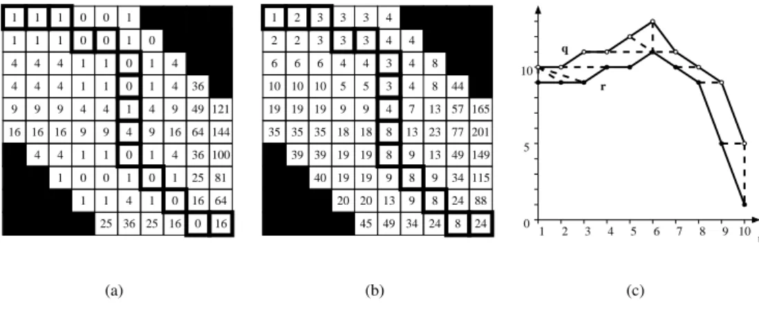
Figure 3 shows the case where m has been set to 5 in the example of Fig. 2. Since the unconstrained optimal warping path was not visiting the black cells of L, this path is identical to that in Fig. 2. So is the DTW distance
D(q, r, w⋆). t 0 16 64 16 0 16 25 36 25 r q 10 5 0 5 6 7 8 9 10 4 3 2 1 1 2 3 3 3 4 2 2 3 3 3 4 4 6 6 6 4 4 3 4 4 8 8 44 5 5 3 4 10 10 10 19 19 19 9 9 7 13 13 23 13 8 8 8 8 8 9 9 24 24 24 9 9 18 18 19 19 19 19 20 20 35 35 35 39 39 13 34 40 49 45 34 49 57 77 165 201 149 115 88 1 1 1 1 1 1 1 1 1 1 1 0 0 1 1 0 0 0 1 4 4 4 4 4 4 4 4 0 0 36 9 9 9 9 9 9 9 4 4 4 4 1 16 16 16 16 49 121 64 144 4 4 1 1 1 0 0 1 1 0 0 4 1 36 25 81 100 1 1 4 1 (a) (b) (c)
Figure 3: DTW with Sakoe-Chiba band: local distance matrix L (a), accumulated distance matrix ∆ (b), query and reference plots with warped pairs (c)
In this work, the Sakoe-Chiba band was not used to bound the maximum time difference between any two associated points, but only to avoid useless computations in regions of L that are not likely to be visited by any optimal path. For instance, for long curves spanning a time interval T of a few minutes, τmax was set to
30 seconds. Clearly, this choice is problem dependent and some tuning is required if computational effort is an issue.
2.3
Practical uses of DTW distance and optimal warping path
Although it makes sense to minimize D(q, r, w) to identify the optimal warping path between two time-series, the value of D(q, r, w⋆) by itself may not be a meaningful measure of their proximity. For instance, if a larger
number of points is used for the comparison, the value of D(q, r, w⋆) will increase accordingly. To deal with this
situation, it sounds more appropriate to consider the normalized DTW distance:
δ = √∑N k=1ℓwk N = D(q, r, w⋆) √ N (14)
If the two curves are smooth enough compared to the sampling period, a higher sampling will lead to a higher value of N but one can expect δ to be few affected.
Further practical information can be obtained from the optimal warping path. With the pairs of indices in w⋆ denoted as in (4), we define the vector of curve offsets as:
y = [qi1− rj1, qi2− rj2, . . . , qiN − rjN] (15)
and the vector of time shifts as:
x = [ti1− tj1, ti2− tj2, . . . , tiN − tjN] (16)
The differences between the two curves can be measured by:
• the average curve offset:
µ = ∑N k=1[y]k N = 1 N N ∑ k=1 (qik− rjk) (17)
• the standard deviation of the curve offsets: σ =
√∑N
k=1([y]k− µ)2
N (18)
• the average time shift:
τ = ∑N k=1[x]k N = 1 N N ∑ k=1 (tik− tjk) (19)
For instance, when comparing two time-series, a small value of µ indicates that, with a proper deformation of the time axes, the curves coincide on the average. τ characterizes the average delay corresponding to that deformation. When comparing several queries to a reference, a larger value of σ denotes more “volatility” with respect to that reference. In case of oscillatory responses, for instance, a small σ indicates that both curves have similar damping.
3
Improvements of the DTW distance
3.1
Extending the method to open-end DTW
The DTW method was initially developed for speech recognition applications where the signals to be compared start and end at zero values. In power system applications where simulations (or simulations and measurements) have to be compared, it is reasonable to assume that the two curves start from steady-state values. However, they may eventually evolve into system instability, in which case they will end in the middle of transients caused by either a monotonic collapse or by growing oscillations.
In such situations, it may not be meaningful to impose the optimal warping path to involve all the n points of each curve. Indeed, under the effect of the above mentioned transients, D(q, r, w⋆), µ or σ may be significantly
and falsely influenced by the last points of the curves. This is even more true in a collapse simulation where the model accuracy is questionable in those degraded operating conditions and, hence, less importance should be given to the final values.
This motivates a modification of the method referred to as open-end DTW, which gives better performances than the standard DTW algorithm [4], allowing only a partial alignment of the time-series thanks to a softening of the Boundary condition defined in Section 2.1.
Thus, instead of requesting the optimal warping path to end up with wN = (iN, jN) = (n, n), it is allowed to
end up in wN = (iN, jN) with:
n′− m′ ≤ iN ≤ n
n′− m′ ≤ jN ≤ n
(jN − n)(iN − n) = 0
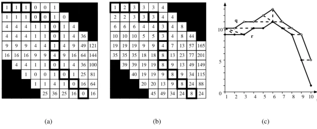
where the equality forces the last point of at least one of the two curves to be involved in the DTW distance. Figure 4 shows an example of open-end DTW. In this case m′has been set 5. As a result, the optimal warping path stops in the (10, 9) entry of L instead of (10, 10) as in Figs. 2 and 3. It is easily seen from Fig. 4.c that from
t = 6 to t = 10, the query curve is delayed with respect to the reference, and therefore does not go as low as the
latter, although the “plunging” evolution is reproduced. The optimal warping path does not involve the last point of the reference curve. This leads to a the DTW distance D(q, r, w⋆) =√8 = 2.828. This value is significantly
smaller than the DTW distance of 4.899 obtained under strict boundary condition. This smaller distance reflects the better matching between both curves when ignoring the last point of the reference time-series.
t 8 7 6 5 0 5 10 q r 25 36 25 16 0 16 64 16 0 1 4 1 1 100 81 25 36 1 4 0 0 1 1 0 0 1 1 1 4 4 144 64 121 49 16 16 16 16 1 4 4 4 4 9 9 9 9 9 9 9 36 0 0 4 4 4 4 4 4 4 4 1 1 0 0 0 0 0 1 1 1 1 1 1 1 1 1 1 1 1 88 115 149 201 165 77 57 49 34 45 49 40 34 13 39 39 35 35 35 20 20 19 19 19 19 18 18 9 9 24 24 24 9 9 8 8 8 8 8 13 23 13 13 7 9 9 19 19 19 10 10 10 4 3 5 5 8 44 8 4 4 3 4 4 6 6 6 4 4 3 3 3 2 2 4 3 3 3 2 1 1 2 3 4 9 10 (a) (b) (c)
Figure 4: Open-end DTW: local distance matrix L (a), accumulated distance matrix ∆ (b), query and reference plots with warped pairs (c)
Similarly to m, and re-using the notation of Section 2.2, m′can be taken as m′ = τmax′ /h where τmax′ is the
largest acceptable time difference on the last pair of associated points.
3.2
Penalizing large time warps
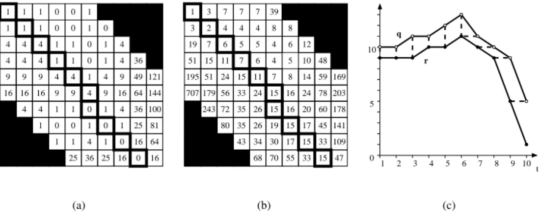
It has been noticed that on some occasions, the DTW algorithm “over-warps” the time axes during its optimization process. This happens in the form of a single point of one time-series being mapped to a large number of points of the other time-series, and was referred to as a singularity in [5]. In Figs. 2, 3 and 4, for instance, the 6th point of the reference curve is a significant singularity in so far as it is mapped to 5 points of the query curve.
Several methods have been proposed to alleviate this problem [5]. In this work, a modification of the slope-weighting technique described in [3] was found sufficient to remove or decrease the importance of singularities.
A singularity corresponds to several steps taken successively in the delay-forward (respectively the forward-delay) direction. Let us denote by kdf the number of steps taken consecutively in the delay-forward direction
and by kf dits counterpart in the forward-delay direction. kdf is reset to zero as soon as a forward-forward or a
matrix are modified as follows: [∆]1j = j ∑ k=1 pk−1[L]1k j = 1, . . . , n (20) [∆]i1 = i ∑ k=1 pk−1[L]k1 i = 2, . . . , n (21) [∆]ij = min{[∆]i−1,j−1+ [L]ij, [∆]i,j−1+ pkdf[L] ij, [∆]i−1,j+ p kf d[L] ij} i, j = 2, . . . , n(22)
where p≥ 1. Thus, the pkdf and pkf dfactors penalize successive mappings that involve a single point of the same
curve. The choice of p may require some tuning as it is problem and sampling dependent. As a rule of thumb, in case of a uniform sampling with time step h, and assuming that a singularity with cumulated delay ∆dis to be
penalized with a factor P ≥ 1, the recommended value is :
p = Ph/∆d
Note that the larger p, the closer the optimal warping path to the diagonal of ∆ and hence, the closer the DTW distance to the Euclidean one.
Figure 5 shows an example of application of the slope-weighted DTW. In this example, the “large” value p = 2 was chosen to highlight the slope-weighting effect: as expected, it yields a nearly-diagonal warping path. The mapping of points is shown in Fig. 5. Under the effect of penalties, the singularity of the 6th point of the reference curve has decreased, since it is now mapped to only two points of the query curve. The corresponding DTW distance is√∑Nk=1ℓwk= 3.873. t 45 33 15 169 203 178 141 109 47 1 1 1 1 1 1 1 1 1 1 1 0 0 1 1 0 0 0 1 4 4 4 4 4 4 4 4 0 0 36 9 9 9 9 9 9 9 4 4 4 4 1 16 16 16 16 49 121 64 144 4 4 1 1 1 0 0 1 1 0 0 4 1 36 25 81 100 1 1 4 1 0 16 64 16 0 16 25 36 25 r q 10 5 0 5 6 7 8 9 10 4 3 2 1 6 2 1 3 7 7 7 39 4 4 4 3 8 8 19 7 5 5 4 6 12 51 15 11 195 707 51 179 243 24 56 72 80 7 15 33 35 35 43 6 11 24 26 26 34 68 4 7 15 15 19 30 70 5 8 16 16 15 17 55 10 14 24 20 17 15 33 48 59 78 60 (a) (b) (c)
Figure 5: Slope-weighted DTW: local distance matrix L (a), accumulated distance matrix ∆ (b), query and reference plots with warped pairs (c)
4
Discussion
4.1
Metric aspects
A desirable property for a measure of distance is that it is a “metric”, which requires to satisfy the following four conditions (the dependency on w⋆is dropped for simplicity of writing):
• Non-negativity: D(q, r) ≥ 0. • Symmetry: D(q, r) = D(r, q).
• Identity of indiscernibles: D(q, r) = 0 ⇐⇒ q = r. • Triangle inequality: D(q, q′) + D(q′, r)≥ D(q, r).
It is easily checked that the first two properties hold true for the DTW distance. On the other hand, it is easily verified with counterexamples that it does not satisfy the last two properties.
In the speech recognition problem, the task is to compare the query (a spoken word) with many references (all word prototypes in a dictionary) to identify the closest to the query (the most likely spoken word). In that problem and, in general, in search algorithms, a measure with metric properties would allow finding the sought reference without computing the DTW distances between the query and all references, which could be computationally demanding, especially with a large number of references.
For the power system applications reported in this paper, however, the absence of a metric structure is not prob-lematic at all, since our purpose is somewhat opposite: determine which of the queries is the closest approximation of a single reference.
While no study has been carried on about loose satisfaction of metric properties in the power system case, empirical evidence of quasi-metric properties was given in a speech recognition problem [10].
4.2
Sampling effects
A possible weakness of the DTW distance is its dependence on the curve sampling. Different samplings may lead to quite different results. For instance, consider the following continuous-time evolutions:
r(t) = t
sampled to get the time-series q and r. Clearly, with an integer sampling period, starting at t = 0, D(q, r, w⋆) = 0
while with any other sampling D(q, r, w⋆)̸= 0.
Algorithms for continuous dynamic time warping have been proposed [6] to deal with this problem, at the cost of increased complexity and computational effort. This paper sticks with the classical, discrete formulation to preserve the intuitiveness and simplicity of the DTW algorithm. The impact of sampling can be reduced by using a small enough sampling period. The resulting computational burden is compensated by storing and processing only the Sakoe-Chiba band in L and ∆.
4.3
Multidimensional DTW
So far it has been considered that the curve comparison involves a set of queries and a single reference. How-ever, since power systems are multi-dimensional systems, it might be of interest to compute a global distance measure between several sets of queries and their corresponding references. To this purpose the concept of multi-dimensional DTW is introduced.
LetS be a set of variables of interest. Note that S should not be too large mainly because involving too many curves exposes to masking effects. For instance, when analyzing the impact of a disturbance on a large power system, it is likely that components far way from its location will respond comparatively less. Involving them in the comparison may “dilute” significant discrepancies on the most affected variables, and potentially give a false impression of accuracy.
For the sake of simplicity, we still suppose that the query qk and reference rk time-series of the same k-th
variable inS span the same time interval and have the same number n of uniformly sampled points. The squared distance between two points of respectively qkand rkis defined, analogously to (2), as:
ℓ(k,i,j)= (qik− r k j)
2 i, j = 1, . . . , n
(23)
The local distance matrix L is redefined as follows:
(L)ij =
∑
k∈S
wkℓ(k,i,j) i, j = 1, . . . , n (24)
where wkis the weight associated to the k-th variable. This weight may account for a conversion between different
higher importance). From there on, the remaining of the procedure detailed in Sections 2.2 and 3, is identical. Therefore, the additional computational effort with respect to the single-dimensional case is very limited, since it has to do with the construction of the L matrix only.
5
Simulation results
This section illustrates the DTW method (and its extension) in two typical applications.
5.1
Solver accuracy comparison
In the first application, the DTW method is used to measure the accuracy of fast, simplified simulation methods. The case has been obtained with the Nordic32 test system documented in [13]. In the scenario of concern, following a line outage, the system undergoes long-term voltage instability under the effect of overexcitation limiters reducing the field currents of generators and load tap changers attempting to restore the distribution voltage (and hence load powers).
The benchmark evolution has been obtained with the 2nd-order Backward Differentiation Formula (BDF) integration formula, using a step size of 0.05 s. Two simplified simulations have been considered:
• fast solver: following the ideas in [11], the backward Euler method has been used to simulate the same
detailed model as in the benchmark but with a large step size of 0.5 s and an appropriate handling of discrete events as explained in [12]. This approach is denoted by BE in the sequel;
• model simplification: the quasi steady-state approximation of the long-term dynamics has been considered
[9], which consists of decomposing the model into fast and slow dynamics, replacing the former by their equilibrium conditions and integrating the latter with a large step size of 1 s. This yields the fastest but also the more approximate time simulation. This approach is denoted by QSS in the sequel.
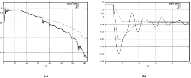
Figure 6.a shows the time evolution of a representative bus voltage obtained by the benchmark (solid lines) and the two simplified (dashed and dotted, respectively) simulation methods. A zoom on the first 10 s is provided in Fig. 6.b. As can be seen, BE overlooks some of the oscillations but matches the benchmark once the large transients have died out. QSS reproduces the same pattern but with a delay that increases towards the end.
0.85 0.9 0.95 1 0 20 40 60 80 100 120 140 t (s) (pu) BENCHMARK BE QSS 0.94 0.95 0.96 0.97 0.98 0.99 1 1.01 1.02 0 2 4 6 8 10 t (s) (pu) BENCHMARK BE QSS (a) (b)
Figure 6: Voltage instability scenario: long-term evolution of voltage (a) and zoom over the first 10 s (b)
To compute the DTW distance, all curves have been sampled every 0.05 s, which is the smallest integration step size (used to obtain the reference curve). Linear interpolation has been used to sample the BE and QSS curves. For easier comparisons with DTW, we consider the normalized Euclidean distance:
ϵ =E(q, r)√
(n) (25)
This distance is found to be ϵ = 3.499× 10⁻³pu for BE and ϵ = 24.45× 10⁻³pu for QSS, which would suggest that QSS is nearly one order of magnitude less accurate than BE.
The DTW distances show that in fact the QSS simulation is not so inaccurate, but just suffers from a growing delay, as can be concluded from a visual inspection of the curves. The DTW measures have been computed with
τmax= τmax′ = 30 s (which corresponds to m = m′= 600) and p = 1.5. The results are summarized in Table 1.
Table 1: solver accuracy comparison; collapse scenario (all values in pu of voltage)
solver δ µ σ τ
BE 1.876× 10⁻³ 0.132× 10⁻³ 1.872× 10⁻³ 0.769 QSS 3.537× 10⁻³ 0.495× 10⁻³ 3.503× 10⁻³ 11.19
The values of δ show that QSS is only twice as inaccurate as BE. µ indicates that QSS suffers from a positive offset larger than BE. The BE curve is characterized by a smaller value of σ because it reproduces part of the
initial voltage dip while the QSS curve goes directly to the underlying equilibrium, as can be seen in Fig. 6.b. τ confirms that QSS suffers from a large average delay.
The simplified solvers considered here are not aimed at reproducing the electromechanical oscillations [11]. However, a slightly more accurate simulation can be obtained - with little additional computational effort - by resorting to the second-order BDF integration scheme instead of Backward Euler (which is first-order BDF), while still keeping the large step size of 0.5 s. This approach is denoted by BDF2 in the sequel.
The respective accuracies of BE and BDF2 with respect to the benchmark have been determined for the curves in Fig. 7, showing the short-term evolution of the active power produced by a generator, in response to another line outage in the Nordic32 system. As can be seen, BDF2 partly reproduces the oscillations while BE just sketches the first swing.
900 950 1000 1050 1100 1150 0 2 4 6 8 10 t (s) (MW) BENCHMARK BDF2 BE
Figure 7: Oscillatory responses to be compared
The normalized Euclidean distances defined by (25) are ϵ = 47.23 MW for BDF2 and ϵ = 43.65 MW for BE which would suggest that both solvers are quite inaccurate, and paradoxically, BDF2 is the least accurate.
The DTW measures have been computed with τmax = τmax′ = 5 s (which corresponds to m = m′ = 100)
and p = 1.5. The results, in MW, are given in Table 2. Unlike the Euclidean distances, the δ values indicate that BDF2 is more accurate, which confirms the observation that, in spite of its high damping, BDF2 still reproduces an oscillation, which is overlooked in the BE response. The µ values indicate that both solvers suffer from a negative offset, while the σ values show that BDF2 has damping closer to the reference than BE. The τ values indicate that BE suffers from an average delay twice as large as BDF2.
Table 2: Solver accuracy comparison; oscillatory scenario (all values in MW)
solver δ µ σ τ
BDF2 27.94 −1.085 27.99 1.077 BE 34.09 −0.547 34.17 2.043
5.2
Model accuracy comparison
We now illustrate how the DTW method can be used to validate the outputs of models with respect to time responses measured on the real system.
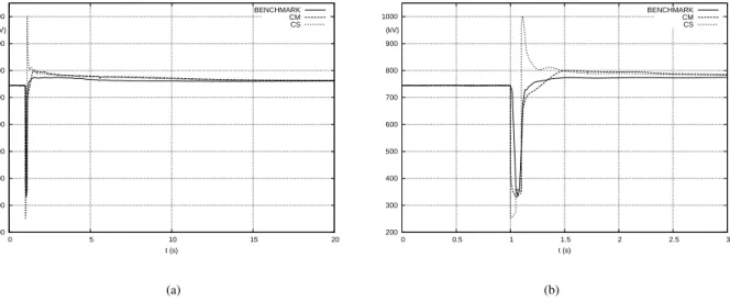
The case relates to a three-phase fault that occurred in 2010 on the 315-kV network of Hydro-Qu´ebec, when energizing a transformer. The fault was cleared in 6 cycles, while some load spontaneously tripped after 3 cycles. The recorded voltage evolution at a 735-kV bus is shown with solid line in Fig. 8. The sampling period is 1 cycle at 60 Hz (≃ 0.0167 s).
Two models were considered when reproducing the event with an industrial software:
• loads wholly represented by a static, exponential model. This model is referred to as CS in the sequel • part of the load represented by an equivalent induction motor. This model is referred to as CM in the sequel.
The simulated response obtained with each model, using a time step size of 0.25 cycle (≃ 0.0042 s) is shown in Fig. 8.a with dashed and dotted lines, respectively. Figure 8.b provides a zoom on the first 3 s.
200 300 400 500 600 700 800 900 1000 0 5 10 15 20 t (s) (kV) BENCHMARK CM CS 200 300 400 500 600 700 800 900 1000 0 0.5 1 1.5 2 2.5 3 t (s) (kV) BENCHMARK CM CS (a) (b)
Clearly, the CS model yields a large voltage spike after fault clearing while the CM model gives results closer to the measurements. Both simulations join the benchmark once the large transients have died out.
To further measure the accuracy of the two models, all curves have been sampled with a period of 0.25 cycle and with linear interpolation. The normalized Euclidean distances in kV are ϵ = 17.59 kV for CM and ϵ = 26.89 kV for CS.
The DTW distances have been computed with τmax= τmax′ = 2.5 s (which corresponds to m = m′= 600)
and p = 1.035. The results are given in Table 3.
Table 3: Model accuracy comparison (all values in kV)
Model δ µ σ τ
CM 9.134 6.806 6.093 1.877
CS 18.17 5.931 17.18 1.976
The respective values of δ show that CM is twice as accurate as CS. µ indicates that both models suffer from a positive offset. σ shows that CM has a damping closer to the reference than CS. τ indicates that both models have a delay around 2 s.
6
Conclusion
A measure of proximity of time-series stemming from power system simulations and/or measurements has been proposed in this paper. This measure is based on Dynamic Time Warping, an algorithm originally developed for speech recognition and now used in several fields. This algorithm warps the time axis and maps the points of both curves to minimize the sum of their squared ordinate differences. This is equivalent to determining the deformation of the time axes which brings the two time-series as close as possible in the Euclidean-norm sense. An efficient dynamic programming algorithm is used for the minimization. Extensions and adaptations of the classical method, to deal with typical power system responses have been presented, together with statistics allowing to characterize the proximity of two time evolutions with as few as 3 parameters: µ, τ and σ. A key point
of any proposed metric is how well it correlates with expert opinion. A further validation of the DTW approach could be obtained by comparing the DTW-based ranking of a set of queries with the ranking made by a power system expert. Depending on the application, the most significant ranking would be based on µ, τ or σ. A multi-dimensional extension allowing system-wide measures of similarity has been also discussed. The effectiveness and usefulness of the method has been demonstrated on several power system applications. The relative accuracy of a set of simplified simulations with respect to a reference was computed on a small system. In the context of model validation, two simulated responses were compared to a recorded measurement of a real incident.
Acknowledgement
This work was performed in the context of the PEGASE project [14] funded by European Community’s 7th Framework Programme (grant agreement No. 211407).
References
[1] Schwer, L.E.: ‘Validation metrics for response histories: perspectives and case studies’, Engineering with Computers, Oct. 2007, Vol. 23, Issue 4, pp. 295-309
[2] Vintsyuk, T.K.: ‘Speech discrimination by dynamic programming’, Kibernetika (in Russian), 1968, Vol. 4, No. 1, pp. 81-88
[3] Sakoe, H., and Chiba, S.: ‘Dynamic programming algorithm optimization for spoken word recognition’, IEEE Trans. on Acoustics, Speech, and Signal Processing, Feb. 1978, Vol. 26, No. 1, pp. 43- 49
[4] Tormene, P., Giorgino, T., Quaglini, S., and Stefanelli, M.: ‘Matching incomplete time series with dy-namic time warping: an algorithm and an application to post-stroke rehabilitation’, Artificial Intelligence in Medicine, Jan. 2009, Vol. 45, Issue 1, pp. 11-34
[5] Keogh, E.J., and Pazzani, M.J.: ‘Derivative dynamic time warping’, Proc. 1st SIAM International Confer-ence on Data Mining, Chicago, USA, Apr. 2001, pp. 1-11
[6] Efrat, A., Fan, Q., and Venkatasubramanian, S.: ‘Curve matching, time warping, and light fields: new algorithms for computing similarity between curves’, Journal of Mathematical Imaging and Vision, Apr. 2007, Vol. 27, No. 3, pp. 203-216
[7] Youssef, A.M., Abdel-Galil, T.K., El-Saadany, E.F., and Salama, M.M.A.: ‘Disturbance classification utiliz-ing dynamic time warputiliz-ing classifier’ IEEE Trans. Power Delivery, Jan. 2004, Vol. 19, No. 1, pp. 272-278
[8] Kong, Y., and Liu, S.: ‘Power System Transient Stability Assessment Based on Geometric features of Dis-turbed Trajectory and DTW’, Proc. 6th International Conference on Natural Computation (ICNC 2010), Yantai, China, Aug. 2010, pp. 485-489
[9] Van Cutsem, T., and Vournas, C.: ’Voltage Stability of Electric Power Systems’ (Kluwer Academic Publish-ers - now Springer, 1998)
[10] Vidal Ruiz, E., Casacuberta Nolla, F., and Rulot Segovia, H.: ‘Is the DTW distance really a metric? An algorithm reducing the number of DTW comparisons in isolated word recognition’, Speech Communication, Dec. 1985, Vol. 4, Issue 4, pp. 333-344
[11] Fabozzi, D., and Van Cutsem, T.: ‘Simplified time-domain simulation of detailed long-term dy-namic models’, Proc. IEEE PES General Meeting, Calgary, Canada, July 2009, pp. 1-8. Available at http://ieeexplore.ieee.org (DOI 10.1109/PES.2009.5275463) and http://hdl.handle.net/2268/9524
[12] Fabozzi, D., Chieh, A.S., Panciatici, P., and Van Cutsem, T.: ‘On simplified handling of state events in time-domain simulation’, accepted for presentation at the 17th Power System Computation Conference (PSCC), Stockholm, Sweden, Aug. 2011, pp. 1-9. Available at http://hdl.handle.net/2268/91650
[13] Glavic, M., and Van Cutsem, T.: ‘Wide-Area Detection of Voltage Instability From Synchronized Phasor Measurements. Part II: Simulation Results’, IEEE Trans. Power Syst., Aug. 2009, Vol. 24, No. 3, pp. 1417-1425