1
Preprint, the final version, of the article that has been transferred to the journal's production team. The citation is:
Mustafa, A., Saadi, I., Cools, M., & Teller, J. (2018). “A Time Monte Carlo method for addressing uncertainty in land-use change models.” International Journal of Geographical Information Science, 1-17. https://doi.org/10.1080/13658816.2018.1503275
A Time Monte Carlo method for addressing uncertainty in land-use
change models
Abstract: One of the main objectives of land use change models is to explore future land use patterns. Therefore, the issue of addressing uncertainty in land use forecasting has received an increasing attention in recent years. Many current models consider uncertainty by including a randomness component in their structure. In this paper, we present a novel approach for tuning uncertainty over time, which we refer to as the Time Monte Carlo (TMC) method. The TMC uses a specific range of randomness to allocate new land uses. This range is associated with the transition probabilities from one land use to another. The range of randomness is increased over time so that the degree of uncertainty increases over time. We compare the TMC to the randomness components used in previous models, through a coupled logistic regression-cellular automata model applied for Wallonia (Belgium) as a case study. Our analysis reveals that the TMC produces results comparable with existing methods over the short-term validation period (2000-2010). Furthermore, the TMC can tune uncertainty on longer-term time horizons, which is an essential feature of our method to account for greater uncertainty in the distant future.
Keywords: land use allocation; uncertainty, stochastic disturbance; Monte Carlo simulation; cellular automata.
2
1. Introduction
One of the primary goals of land use change models is to forecast possible future land states. Although uncertainty is an inherent feature of any forecast, few land use change models consider uncertainty as a component of the model structure. Because predicting future land use pattern is difficult, land use change models can be regarded as
exploratory tools to assist in the decision making by exploring various scenarios. Pontius and Neeti (2010) discuss two contrasting views concerning the role of
uncertainty in scenario-based analysis. One view considers that uncertainty is irrelevant to scenario-based analysis because storylines are not predictive. Some studies have simulated future land use change without accounting for uncertainties (e.g. Poelmans et al., 2010). The other view considers that uncertainty is important in scenario-based analysis which takes into account the link between the qualitative storyline and its quantitative expression. Following this second view, our study proposes a method that can be applied to account for uncertainties.
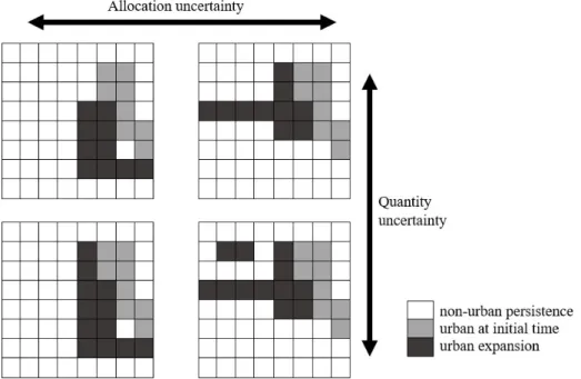
In a comprehensive review of 114 land use change applications, van Vliet et al. (2016) found that only 17% of the reviewed applications addressed uncertainty. Uncertainties may arise from many sources. Pontius and Neeti (2010) identified three groups of such sources: the data, the model, and future land change simulation. First, errors in the model’s input data are likely to exist and have been investigated in some studies (e.g. Tayyebi et al., 2014). Second, the construction of the model may contain uncertainty associated with its algorithms (Pontius and Neeti, 2010). Third, future simulation involves two main types of uncertainty, namely the estimation of the future change amount (quantity uncertainty) and the spatial allocation of land use changes. Figure 1 depicts the difference between quantity uncertainty and spatial allocation uncertainty.
3
The quantity uncertainty is captured in many land use models by simulating various scenarios that differ in the quantity of change (e.g., Cammerer et al., 2013; Landuyt et al., 2016). The spatial allocation uncertainty is associated with the potential
nonstationary character of the spatial distribution of land use types. Generally, land use models extrapolate calibrated allocation results to simulate future landscape. Thus, these models implicitly assume that the calibrated parameter set is valid for the future and do not consider the nonstationary features of the land use allocation related to the political, economic, and/or environmental conditions that are known to be nonstationary (van Vliet et al., 2016). Our main focus in the present study is related to the spatial allocation uncertainty. The uncertainty in the allocation process has been addressed in some studies using fuzziness (e.g., Wang et al., 2013) or randomness by introducing a stochastic component (e.g., Yang et al., 2008). The randomness ensures that each run can produce a different land use pattern and that some patterns can be accurate by chance (Brown et al., 2005; van Vliet et al., 2016). Some of the current techniques for embedding allocation uncertainty in land use change models incorporate a stochastic
Figure 1. Quantity and spatial allocation uncertainties in land use change models. The quantity of change in the first and second cases, the vertical direction, is 10 and 12 respectively. In each case, the quantity of change is allocated differently, the horizontal direction.
4
disturbance (SD) term or a Monte Carlo simulation (MC) method. Feng (2017) and Yang et al. (2008) introduced an SD term, after White and Engelen (1993), whereas Li and Liu (2006), Liu et al. (2008), and Wu (2002) used an MC method in their models to consider uncertainty.
The primary goal of this paper is to tune the degree of allocation uncertainty over time so that the uncertainty degree varies between the immediate future and the distant future. Our approach, following Wu (2002), compares the transition probability from one land use state to another in each land unit with a random number. However, a major difference of our work lies in generating a uniform random number drawn over a
dynamic range associated with transition probabilities from one land use state to another, and this range increases over time.
We incorporate our method in a cellular automata (CA) model to simulate urban expansion in Wallonia (Belgium) for two time-intervals: the calibration interval 1990-2000, and the validation interval 2000-2010. After calibrating and validating the model, we compare the results obtained by our method and those by the two most widely used methods, SD and MC. The comparison demonstrates the robustness of our method against SD and MC methods.
The paper is structured as follows. In section 2, we review SD and MC methods and then describe our method. Section 3 presents the land use change model, study area, and data. In section 4, we show and discuss our results. Section 5 presents our conclusions.
2. Modeling spatial allocation uncertainty
In this section, we review the SD method proposed by White and Engelen (1993) and the MC method proposed by Wu (2002) for incorporating uncertainty into land use change models. Thereafter, we introduce the proposed method, the Time Monte Carlo
5
(TMC) method. Once the transition probability has been computed for each landscape unit, the SD term perturbs each probability score in its vicinity by a random number that can be calculated as follows (White and Engelen, 1993):
𝑆𝐷 = 1 + (− ln 𝛾) (1)
where γ is a uniform random number between 0 and 1, and σ is a parameter that allows control of the magnitude of the SD. When σ is set at 0, the model behaves
deterministically. In contrast, when σ is set at high positive values, the model follows a random process. Introducing an SD term in the transition probabilities may bias the model outcomes because cells with very low transition probabilities would be able to change their state (García et al., 2011; Wu, 2002). Wu (2002) proposed an alternative method that employs an MC procedure for modeling spatial allocation uncertainty. In this approach, after computing the transition probabilities, a cell in the landscape is randomly selected, its probability is compared with a random number uniformly distributed between 0 and 1, and the state of a cell will change if its probability score is greater than the generated random number. One of the shortcomings of this approach is that it does not allow control of the degree of randomness. Therefore, Wu (2002) transformed the transition probability of each cell by comparing it with the largest available probability at each time-step, as follows:
𝑃𝑖′ = 𝑃𝑖 exp [−𝛿(1 − 𝑃𝑖 /max (𝑃 )] (2)
where Pi’t is the updated transition probability for cell i at time-step t, Pit is the original
probability, δ is a dispersion term, and max(Pt) finds the maximum transition
probability at time-step t. The dispersion term, δ, in Eq. 2 plays a role equivalent to σ in Eq. 1. When δ is set to high values, transition probabilities decrease away from the
6
maximum probability at each time-step, in particular for cells with a lower probability score. Thus, a distinct difference results between cells with higher probabilities and those with lower probabilities, and there will be less chance for land use change in cells with lower probabilities.
Although the two methods explained above are widely used to model the spatial allocation uncertainty, neither method ensures that the degree of uncertainty can vary over time. In reality, the distant future involves more uncertainty about aspects such as the economic value of land, available communication means, and social/household preferences. All these aspects play a key role in land allocation and become less predictable into the distant future. A few studies have attempted to demonstrate the increase in uncertainty as a model simulates land use change further into the future (e.g., Pontius et al., 2006; Pontius and Neeti, 2010). Our study is one of the first studies that propose a Monte Carlo process to increase the degree of uncertainty over time in land use change modeling.
The proposed TMC method uses an MC procedure as in Wu (2002). At each time-step, a cell is selected at random, and its computed transition probability is compared with a uniform random number within a dynamic range. The proposed method is distinguished from the method of Wu (2002) is that Wu defines this range between the minimum and maximum probabilities, i.e., 0 and 1. We set this range variable to allow tuning the degree of uncertainty over time. At each time-step, the computed transition probabilities are sorted in a descending order, with the most suitable cell at the top of the list.
Typically, the top-scoring cells from the sorted list change their state until they meet the requested change quantity. To consider uncertainty, the model randomly selects one cell in a set of cells with the largest probabilities. The size of this set of the cell is initially determined by the quantity of change and subsequently increased to include more cells.
7
Thereafter, the model compares the transition probability of the selected cell to a uniform random number and the cell changes its land use state according to the following equation:
𝑆𝑖 = 𝑐ℎ𝑎𝑛𝑔𝑒, 𝑃𝑖 > 𝑟𝑎𝑛𝑑 𝑛𝑜𝑛 − 𝑐ℎ𝑎𝑛𝑔𝑒, 𝑜𝑡ℎ𝑒𝑟𝑤𝑖𝑠𝑒
(3)
where Sit+1 is the state of the cell i at the next time-step, Pit is the computed transition
probability at time-step t, and rand is a uniform random number between randmax and randmin. We set rand_max and rand_min as follows:
𝑟𝑎𝑛𝑑 = max(𝑃 ) ,
𝑟𝑎𝑛𝑑 = 𝑡𝑟𝑎𝑛𝑠(𝑞 + (𝑡 × ɸ × 𝑞))
(4)
where max(Pt) returns the maximum probability at time-step t; and trans(q+(t×ɸ×q))
returns the transition value of a cell during time-step t from the sorted list whose location is determined by q, the change quantity per time-step, and ɸ is a specific percentage of q. In this way, the model behaves deterministically at the beginning but slowly behaves more stochastically as the model operates over time.
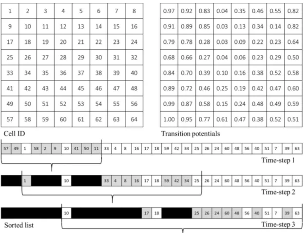
Figure 2 illustrates an example of the method. In this example, the model sorts the cell values in a descending order according to their transition probabilities. Assuming that q=8 and ɸ=25%, the model randomly selects 8 cells out of 10 (Figure 2 from the sorted cells list in time-step 1), 8 cells out of 12, and 8 cells out of 14 in time-steps 1, 2, and 3, respectively. The cells that are converted to another land use are selected by comparing the transition probability with a random number according to Eq. 3.
8
3. Land use change model
In this study, we apply a grid-based CA land use change model to simulate the gain of the urban category in Wallonia (Belgium), as a case study, between 1990 and 2010. Urban land use maps of 1990 and 2000 are used to calibrate the model parameters. The calibrated parameters are then used to simulate the spatial allocation of the 2000-2010 urban gain. We validate the model by comparing the simulated urban gain during 2000-2010 with the observed urban gain during 2000-2000-2010. The model has two main
modules: the demand module and the allocation module. Our emphasis is not on the quantity uncertainty, but rather on the allocation uncertainty, and therefore we assume that the annual demand for increasing urban land is the same from 1990-2000 (for calibration) and from 2000-2010 (for validation) divided by 10 (the number of years).
Figure 2. Example of the TMC method. White: no-change, gray: changes done in the current time-step, and black: changes done in the previous time-septs.
9
The allocation module allocates new urban cells based on transition probabilities. Two major components shape the transition probabilities following the approaches by
Mustafa et al. (2018a), Poelmans and Van Rompaey (2010), and Wu (2002). The first is based on a set of urbanization driving forces. The second component concerns the dynamic interaction between neighborhood land uses. The transition probability P for cell i at time-step t is computed as follows:
t (.)t
d n
Pi Pi Pi con (5)
where (Pid) is the urbanization probability based on urbanization driving forces, (Pin)t is
the neighborhood interaction, and con(.) is restrictive conditions for land use change. The (Pid) is calculated as:
(𝑃𝑖 ) = exp(𝛽 + 𝛽 𝜒 + 𝛽 𝜒 + ⋯ + 𝛽 𝜒 )
1 + exp(𝛽 + 𝛽 𝜒 + 𝛽 𝜒 + ⋯ + 𝛽 𝜒 ) (6)
where β0 is the intercept, (X1, X2, …, Xn) are the land use change driving forces and (β1,
β2, . . ., βn) are the weights of the driving forces. A logistic regression model (logit) is
employed to calibrate the weights βn.
(Pin)t is calculated as follows (Feng et al., 2011; Wu, 2002):
( ) 1 t n count s urban Pi n n (7)where count(s=urban) represents the number of urban cells amongst the Moore n×n neighborhood. In each time-step, representing one year, the model converts the non-urban cells according to Eq. 3, until meeting the required change amount.
3.1. Validation
10
allocation accuracy of the model. The validation is done while eliminating the observed urban cells at the initial time-step from the spatial extent. The goodness of fit of the logit model is assessed using the McFadden pseudo R-square (PR²) and the relative operating characteristic (ROC) procedure (Pontius and Parmentier, 2014). The PR² mimics the R-squared statistic of linear regression models. A value of 1 shows a perfect fit; a PR² of 0 indicates a random fit (Mustafa et al., 2018c). The ROC compares the transition probability map, generated with Eq. 6, to a map with the observed changes. It defines a number of cut-off points and calculates the rate of the true-positives and the false-positives at each cut-off point and relates these rates to each other in a graph. The ROC measures the area under the curve (AUC). AUC=0.5 means allocation as good as random and AUC=1 means perfect allocation.
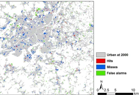
We evaluate the allocation performance by showing the hits (H) indicating that the expansion areas in the observed map were simulated as expansion; misses (M)
indicating that the expansion areas in the observed map were simulated as no-changes; false alarms (FA) indicating that the no-changes in the observed map were simulated as expansion; and correct rejections (CR) indicating that the no-changes in the observed map were simulated as no-changes, following the approaches by Liu et al. (2014) and National Research Council (2014). This evaluation is performed for the urban gain.
3.2. Case study area and model implementation
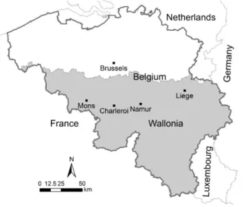
The land use model (section 3) is applied to the Wallonia region (Figure 3). The region occupies 55% of Belgium with an area of 16,844 km2. The urban land use maps for
1990, 2000, and 2010 were produced using Belgian cadastral vector data (CAD) from the Land Registry Administration of Belgium. We rasterized the CAD data at a spatial resolution of 2 m. The rasterized maps were then aggregated to a resolution of 100 m. Each aggregated cell was assigned a density value by counting the number of 2 m cells.
11
The aggregated data were then classified into non-urban with a density < 25 and urban with a density ≥ 25. As the average area of a building in Belgium is about 100 m² (Tannier and Thomas, 2013); a density value of 25, representing an average-sized building of 100 m², is selected to ensure that each aggregated cell has at least one building. The urban configuration in this case study is the entire polycentric urban system, suburbs and rural areas. The data show no loss of urban.
Table 1 lists the driving forces used in the model based on a literature review (e.g. Cammerer et al., 2013; Dubovyk et al., 2011; Poelmans and Van Rompaey, 2010) and the findings of previous work on our study area (e.g. Mustafa et al., 2018a, 2018b).
Table 1. List of the urbanization driving forces.
Factor Name Type Unit
X1 Elevation (DEM) Continuous Meter
X2 Slope Continuous Percent rise
X3 Dist. to RC1 Continuous Meter
X4 Dist. to RC2 Continuous Meter
X5 Dist. to RC3 Continuous Meter
X6 Dist. to RC4 Continuous Meter
X7 Dist. to railway stations Continuous Meter X8 Dist. to large-sized cities Continuous Meter X9 Dist. to med-sized cities Continuous Meter X10 Employment rate Continuous Percent X11 Richness index Continuous Percent
X12 Zoning Categorical Binary (0 non built-up, 1 built-up) Figure 3. The study area – Wallonia.
12
The slope data are generated based on a digital elevation model (DEM) made available by the Belgian National Geographic Institute. Accessibility factors include the
Euclidean distance to roads in 2001, railway stations in 1999, and Belgian cities. Roads are categorized into four classes: RC1 (highways), RC2 (main roads), RC3 (secondary roads), and RC4 (local roads). Large-sized cities represent all Belgian cities with a population > 90,000 in 2000, whereas medium-sized cities are all cities with a population between 20,000 and 90,000 in 2000. The employment rate and richness index in 2000 are used as socioeconomic factors. The zoning map is based on the Wallonia zoning plan adopted between 1977 and 1987. Since 1987, changes in the zoning plan have been very limited in space and size. All zones where urban
development is legally permitted are encoded as 1 and all other zones are encoded as 0. We standardized the driving forces as our aim is to elucidate relationships. To minimize the potential of spatial autocorrelation, which could bias the estimates of parameters in the logit analysis (Overmars et al., 2003), we used a data sampling approach following Poelmans et al. (2010), Cammerer et al. (2013), and Mustafa et al. (2017). A set of 20,000 cells was randomly selected, with an equal number of no-changes and changes. Existing urban cells in 1990 were excluded from the sampling. After 100 runs of the logit model with different sets of samples, we selected the set with the best area under ROC curve (AUC).
4. Results and discussion
In this section, we highlight the result of the logit calibration and discuss the allocation uncertainty. The estimated coefficients of the logit model are shown in Table 2.
The PR² of the logit model is 0.295. Although PR² and R-squared values both range from 0 to 1 with higher values indicating a better fit to the model, PR² values are not equivalent to OLS R-squared values. As the logit model is a maximum likelihood
13
estimation method, the PR² values tend to be considerably lower than the OLS R-squared (McFadden, 1977). Domencich and McFadden (1975) state that PR² range of 0.2-0.4 represents an OLS R-squared values between 0.7-0.9. The AUC for the transition probability map generated by the logit model is 0.833.
Table 2. The logit coefficients.
Factor Name Coefficient β
Intercept -0.9030 X1 Elevation 0.0623* X2 Slope -0.2183* X3 Dist. to RC1 -0.0744* X4 Dist. to RC2 -0.0819* X5 Dist. to RC3 -0.2734* X6 Dist. to RC4 -0.5558*
X7 Dist. to railway stations -0.0042 X8 Dist. to large-sized cities -0.1351* X9 Dist. to med-sized cities -0.1661* X10 Employment rate 0.0003 X11 Richness index -0.0002
X12 Zoning 3.0348*
*Significant at a 95% confidence level
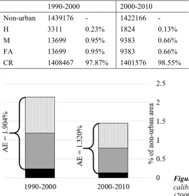
Table 3. Number of cells of hits (H), misses (M), false alarms (FA), and correct rejections (CR) in the non-urban area. 1990-2000 2000-2010 Non-urban 1439176 - 1422166 - H 3311 0.23% 1824 0.13% M 13699 0.95% 9383 0.66% FA 13699 0.95% 9383 0.66% CR 1408467 97.87% 1401576 98.55%
Figure 4. Allocation errors (AE) for calibration (1990-2000) and validation (2000-2010).
14
Table 3 lists total numbers of H, M, FA, and CR in the calibration and validation time intervals. The allocation error (AE), equals M+FA, for the calibration time interval is 1.904% and 1.320% for the validation time interval (Figure 4). We set ɸ in Eq. 4. at 1%, 2%, 10%, 50%, 100%, and 200%. To compare the performance of the TMC with the SD and the MC methods, we examine the model performance with respect to each individual method. The SD is introduced in the model by updating Eq. 5 as follows:
t (.)t
d n
Pi Pi Pi con SD (9) We use different values of σ (Eq.1) to investigate its effect on the model. For the MC method, Wu (2002) suggests that the range of δ is usually 1-10. Accordingly, we set δ at 1, 2, 4, 6, 8, and 10. With higher values of δ, the model tends to produce strongly
skewed probabilities that cause the computation time to increase exponentially. For example, when δ was set at 20 the cells with original probabilities of 0.9426 and 0.5854 become 0.5121 and 0.0002 after implementing Eq. 2. The computing time with a high δ value is long; for instance, one run using δ=15 is ~1.8 h, and one run using δ=20 is ~23.9 h. Table 4 presents the average computation time per run for each method. We implemented our model in MATLAB, running on a desktop computer clocked at 3.60 GHz with 32.0 GB RAM. The results indicate that the TMC method is faster than the SD and the MC methods.
Table 4. The average run-time per run.
Method Run time (seconds)
Deterministic model 5 TMC ɸ = 0.01 (1%) 26 TMC ɸ = 2 (200%) 6 SD σ = 0.01 36 SD σ = 2 30 MC δ = 1 42 MC δ = 10 482
Many simulations are required to investigate the properties of the model in the dynamic environment of different random noises; we therefore ran the model 9,000 times (500
15
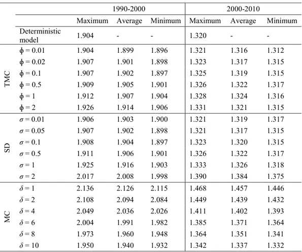
runs per configuration). The simulated allocation error (AE) for new urban cells is given in Table 5. Based on the experimental results, the TMC method with ɸ = 0.01, 0.02, and 0.1 in the model slightly improves the averaged AE. This is also the case for the SD method with σ=0.01 and 0.05. Increases in both ɸ and σ decrease the averaged AE as the model involves more randomness. In contrast, the MC method projects an increase in the averaged AE with higher values of δ as the result that δ controls the exponential curve that scales the transition probability. Consequently, higher δ values cause a more skewed curve, and the chance of cells with higher transition probability values also increases.
Table 5. Allocation error for new urban cells for 9,000 runs.
1990-2000 2000-2010
Maximum Average Minimum Maximum Average Minimum Deterministic model 1.904 - - 1.320 - - T M C ɸ = 0.01 1.904 1.899 1.896 1.321 1.316 1.312 ɸ = 0.02 1.907 1.901 1.898 1.323 1.317 1.315 ɸ = 0.1 1.907 1.902 1.897 1.325 1.319 1.315 ɸ = 0.5 1.909 1.905 1.901 1.326 1.322 1.317 ɸ = 1 1.912 1.907 1.904 1.328 1.324 1.316 ɸ = 2 1.926 1.914 1.906 1.331 1.321 1.315 SD σ = 0.01 1.906 1.903 1.900 1.321 1.319 1.317 σ = 0.05 1.907 1.902 1.898 1.321 1.317 1.315 σ = 0.1 1.908 1.904 1.897 1.323 1.320 1.315 σ = 0.5 1.911 1.906 1.901 1.326 1.322 1.317 σ = 1 1.925 1.916 1.903 1.333 1.326 1.318 σ = 2 2.017 2.008 1.998 1.390 1.384 1.375 M C δ = 1 2.136 2.126 2.115 1.468 1.457 1.446 δ = 2 2.108 2.094 2.084 1.449 1.439 1.432 δ = 4 2.049 2.036 2.026 1.411 1.402 1.393 δ = 6 2.004 1.991 1.982 1.385 1.371 1.364 δ = 8 1.973 1.960 1.948 1.364 1.351 1.341 δ = 10 1.950 1.940 1.932 1.342 1.337 1.332
Figure 5 presents H, M, and FA for the validation time interval for the deterministic model.
16
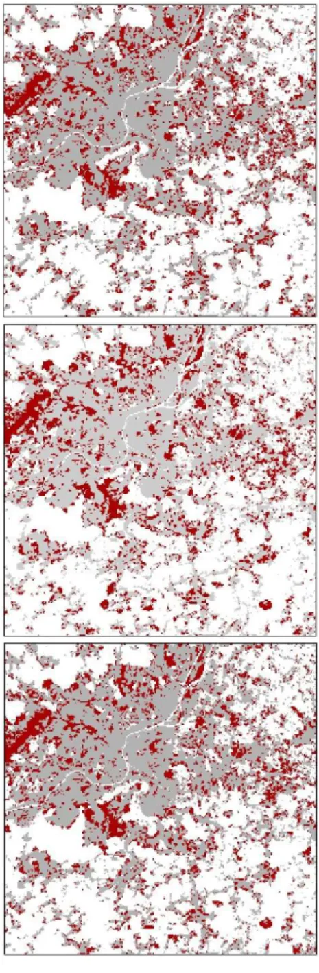
Figure 6 illustrates the future urban patterns for 2030 and 2100. We set a fixed
simulated quantity per time-step, one year, equal to the observed quantity during 2000-2010 divided evenly by 10. Figure 6 demonstrates that the MC method cannot produce simulations similar to the results from deterministic model. Furthermore, this
comparison becomes more difficult with lower values of δ. In contrast, the SD method with a very low degree of σ produces simulations that are similar, with some marginal differences, to results from deterministic model, which can be expected as the model tends to evolve to a stable state with lower degrees of σ. By increasing the degree of σ, the model produces simulations that are quite different from those produced in a deterministic way. Figure 6 confirmed that the proposed TMC method inherits well the randomness in the model. The TMC model produces simulations that are similar, with marginal differences, to the results from deterministic model at the earlier time-steps (e.g., 2030) and tunes the simulations far from the deterministic-based simulations as the model simulates further into the future (e.g., 2100). One could ask why the SD method is not used to tune uncertainty over time since it produces comparable results with the TMC method, and we can increase the degree of randomness over time via σ.
17
A key feature of the TMC method is that the TMC keeps the original transition
probabilities, which is not the case with the SD method. Retaining the original transition probabilities enables retrospection of the land use change process in which the
landowners may resort to speculative motives for hoarding land, in anticipation of the potential urban development in the future. Regarding the magnitude of uncertainty, which is controlled by ɸ or σ, Table 6 shows that the TMC method controls the degree of randomness more efficiently than the SD method.
2030 2100 O ri gi na l m od el T M C | ɸ = 0 .0 1 SD | σ = 0 .0 1
18 SD | σ = 2 M C | δ = 1 0 M C | δ = 1
Table 6. Percentage of simulated urban gain allocated differently in the 500 simulations for each configuration.
2030 2100
Maximum Average Minimum Maximum Average Minimum TMC | ɸ = 0.01 1.37 1.21 0.99 5.76 5.38 4.96 TMC | ɸ = 2 34.45 33.75 32.99 36.55 36.17 35.78 SD | σ = 0.01 1.35 1.14 0.94 1.05 0.76 0.89 SD | σ = 2 62.06 61.17 60.18 35.72 35.28 34.79 MC | δ = 10 38.64 37.99 37.22 31.59 31.16 30.66 MC | δ = 1 85.70 85.32 84.93 62.44 62.12 61.76
Figure 6. 2030 and 2100 simulations for different configurations for Liege metropolitan.
19
Table 6 gives the number of new cells that were differently allocated between every two runs of the 500 simulations for each configuration. For example, in case of the TMC with ɸ = 0.01 the maximum allocation difference between two runs in 2030 is 1.37%; the model allocates 22107 cells out of 22414 new cells in the same locations in the two runs while allocates 307 cells differently. The table illustrates the dependence of model results on the degree of the randomness parameter. The results reveal that the SD method generates landscape patterns for 2100 that are more similar to each other than the patterns generated for 2030. This is also the case for the MC method. This is against expectations because the distant future is more uncertain than the near future. One explanation for this is that the logit model, based on the factors presented in Table 2, efficiently narrowed the potential areas to be urbanized in the future; thus, the future simulations tended to be similar when reaching the maximum potential values. Both the SD and the MC methods are set at a constant change amount per time-step, whereas the available number of cells that can change their land use state decreases with later time-steps. If the number of available cells is lower, as is the case in 2100, the possibility for the available cells to be randomly selected during each run is higher. In contrast, the TMC method is set at a fixed change amount and the number of cells that can change their state increases with time. As a result, the TMC method is able to increase the degree of randomness over time.
If the simulations are uniform, a specific number of cells will change their state in most of the simulations resulting in lower differences in the allocation process. In contrast, if the simulations are very variable, many cells will change to another state in each simulation, and therefore the difference between each simulation is high. Forecasting and interpreting the future simulations would be challenging if the model generates land use patterns that are very different from each other. With a lower degree of randomness,
20
the SD-based model generates similar landscape patterns in the distant future, such that the future simulations can be considered as an extrapolation of the past trends. The TMC method with ɸ = 0.01 produces patterns with small differences for the near future (e.g. 2030) and greater differences for the distant future. Notably, by 2100, the TMC method is still able to generate patterns that are not very different from each other. Our proposed method assumes that all projections are exposed to the same sources of allocation uncertainty. Therefore, further research is required to examine how to
quantify several sources of spatial allocation uncertainty such as uncertainties related to the model structure, model simplification, and model parameter estimates. For example, our model was calibrated and validated with 1990-2010 data. Throughout this period, there were no major urban transition breaks and the land use dynamics were considered rather consistent over time. In contrast, applying our model to urban land over a distant past, for example, from 1950 to 2010, would allow us to analyze uncertainties related to major development breaks, such as the shift from a train-based to a car-based city in the 1950s and 1960s, the succession of diverging economic cycles, or the adoption of legally binding land use regulation in the late 1970s. Therefore, extension of this study will examine the non-linear type of change and include a longer period in model calibration and validation.
5. Conclusions
We have proposed the Time Monte Carlo method (TMC) to introduce randomness in land use change models with the aim of modeling spatial allocation uncertainty. The method is based on a Monte Carlo simulation in which a cell in the landscape is randomly selected and its transition probability from one land use to another is compared with a random number uniformly distributed within a dynamic range that increases over time. We compared the proposed method with two widely used methods
21
to introduce randomness in land use change forecasting: stochastic disturbance, and Monte Carlo simulation. The three methods were introduced into a logistic regression-cellular automata model that was developed to simulate urban expansion in Wallonia (Belgium) between 1990 and 2010.
Our analysis reveals that the TMC method produces results comparable with the existing methods over the short-term validation period (2000-2010). Furthermore, the proposed method is capable of tuning uncertainty on longer-term horizons. Controlling the degree of randomness over time is an important feature of the TMC method as the distant future is characterized by more uncertainty than the near future.
Acknowledgement: The research was funded through the ARC grant for Concerted Research Actions for project number 13/17-01 financed by the French Community of Belgium (Wallonia-Brussels Federation); and through the European Regional
Development Fund – FEDER (Wal-e-Cities Project).
ORCID
Ahmed Mustafa http://orcid.org/0000-0002-1592-6637
Ismaïl Saadi http://orcid.org/0000-0002-3569-1003
Mario Cools http://orcid.org/0000-0003-3098-2693
Jacques Teller http://orcid.org/0000-0003-2498-1838
References:
Brown, D.G.B.C., Page, S., Riolo, R., Zellner, M., Rand, W., 2005. Path dependence and the validation of agent‐based spatial models of land use. Int. J. Geogr. Inf. Sci. 19, 153–174.
https://doi.org/10.1080/13658810410001713399
Cammerer, H., Thieken, A.H., Verburg, P.H., 2013. Spatio-temporal dynamics in the flood exposure due to land use changes in the Alpine Lech Valley in Tyrol (Austria). Nat. Hazards 68, 1243–1270. https://doi.org/10.1007/s11069-012-0280-8
Domencich, T.A., McFadden, D., 1975. Urban travel demand: a behavioral analysis. North-Holland Publishing Co., Oxford, England.
Dubovyk, O., Sliuzas, R., Flacke, J., 2011. Spatio-temporal modelling of informal settlement
development in Sancaktepe district, Istanbul, Turkey. ISPRS J. Photogramm. Remote Sens., Quality, Scale and Analysis Aspects of Urban City Models 66, 235–246.
https://doi.org/10.1016/j.isprsjprs.2010.10.002
Feng, Y., 2017. Modeling dynamic urban land-use change with geographical cellular automata and generalized pattern search-optimized rules. Int. J. Geogr. Inf. Sci. 31, 1198–1219.
22 Feng, Y., Liu, Y., Tong, X., Liu, M., Deng, S., 2011. Modeling dynamic urban growth using cellular
automata and particle swarm optimization rules. Landsc. Urban Plan. 102, 188–196. https://doi.org/10.1016/j.landurbplan.2011.04.004
García, A.M., Santé, I., Crecente, R., Miranda, D., 2011. An analysis of the effect of the stochastic component of urban cellular automata models. Comput. Environ. Urban Syst. 35, 289–296. https://doi.org/10.1016/j.compenvurbsys.2010.11.001
Landuyt, D., Broekx, S., Engelen, G., Uljee, I., Van der Meulen, M., Goethals, P.L.M., 2016. The importance of uncertainties in scenario analyses – A study on future ecosystem service delivery in Flanders. Sci. Total Environ. 553, 504–518. https://doi.org/10.1016/j.scitotenv.2016.02.098 Li, X., Liu, X., 2006. An extended cellular automaton using case‐based reasoning for simulating urban
development in a large complex region. Int. J. Geogr. Inf. Sci. 20, 1109–1136. https://doi.org/10.1080/13658810600816870
Liu, X., Li, X., Liu, L., He, J., Ai, B., 2008. A bottom‐up approach to discover transition rules of cellular automata using ant intelligence. Int. J. Geogr. Inf. Sci. 22, 1247–1269.
https://doi.org/10.1080/13658810701757510
Liu, Y., Feng, Y., Pontius, R.G., 2014. Spatially-Explicit Simulation of Urban Growth through Self-Adaptive Genetic Algorithm and Cellular Automata Modelling. Land 3, 719–738.
https://doi.org/10.3390/land3030719
McFadden, D., 1977. Quantitative Methods for Analyzing Travel Behaviour of Individuals: Some Recent Developments (Cowles Foundation Discussion Papers No. 474). Cowles Foundation for Research in Economics, Yale University.
Mustafa, A., Cools, M., Saadi, I., Teller, J., 2017. Coupling agent-based, cellular automata and logistic regression into a hybrid urban expansion model (HUEM). Land Use Policy 69C, 529–540. https://doi.org/10.1016/j.landusepol.2017.10.009
Mustafa, A., Heppenstall, A., Omrani, H., Saadi, I., Cools, M., Teller, J., 2018a. Modelling built-up expansion and densification with multinomial logistic regression, cellular automata and genetic algorithm. Comput. Environ. Urban Syst. 67, 147–156.
https://doi.org/10.1016/j.compenvurbsys.2017.09.009
Mustafa, A., Rompaey, A.V., Cools, M., Saadi, I., Teller, J., 2018b. Addressing the determinants of built-up expansion and densification processes at the regional scale. Urban Stud. 0042098017749176. https://doi.org/10.1177/0042098017749176
Mustafa, A., Saadi, I., Cools, M., Teller, J., 2018c. Understanding urban development types and drivers in Wallonia. A multi-density approach. Int. J. Bus. Intell. Data Min. 13, 309–330.
https://doi.org/10.1504/IJBIDM.2017.10004788
National Research Council, 2014. Advancing Land Change Modeling: Opportunities and Research Requirements. https://doi.org/10.17226/18385
Overmars, K.P., de Koning, G.H.J., Veldkamp, A., 2003. Spatial autocorrelation in multi-scale land use models. Ecol. Model. 164, 257–270. https://doi.org/10.1016/S0304-3800(03)00070-X
Poelmans, L., Van Rompaey, A., 2010. Complexity and performance of urban expansion models. Comput. Environ. Urban Syst. 34, 17–27. https://doi.org/10.1016/j.compenvurbsys.2009.06.001 Poelmans, L., Van Rompaey, A., Batelaan, O., 2010. Coupling urban expansion models and hydrological
models: How important are spatial patterns? Land Use Policy 27, 965–975. https://doi.org/10.1016/j.landusepol.2009.12.010
Pontius, R.G., Neeti, N., 2010. Uncertainty in the difference between maps of future land change scenarios. Sustain. Sci. 5, 39. https://doi.org/10.1007/s11625-009-0095-z
Pontius, R.G., Parmentier, B., 2014. Recommendations for using the relative operating characteristic (ROC). Landsc. Ecol. 29, 367–382. https://doi.org/10.1007/s10980-013-9984-8
Pontius, R.G., Versluis, A.J., Malizia, N.R., 2006. Visualizing certainty of extrapolations from models of land change. Landsc. Ecol. 21, 1151–1166. https://doi.org/10.1007/s10980-006-7285-1
Tannier, C., Thomas, I., 2013. Defining and characterizing urban boundaries: A fractal analysis of theoretical cities and Belgian cities. Comput. Environ. Urban Syst. 41, 234–248.
https://doi.org/10.1016/j.compenvurbsys.2013.07.003
Tayyebi, A.H., Tayyebi, A., Khanna, N., 2014. Assessing uncertainty dimensions in land-use change models: using swap and multiplicative error models for injecting attribute and positional errors in spatial data. Int. J. Remote Sens. 35, 149–170. https://doi.org/10.1080/01431161.2013.866293 van Vliet, J., Bregt, A.K., Brown, D.G., van Delden, H., Heckbert, S., Verburg, P.H., 2016. A review of
current calibration and validation practices in land-change modeling. Environ. Model. Softw. 82, 174–182. https://doi.org/10.1016/j.envsoft.2016.04.017
23 Wang, H., He, S., Liu, X., Dai, L., Pan, P., Hong, S., Zhang, W., 2013. Simulating urban expansion using a cloud-based cellular automata model: A case study of Jiangxia, Wuhan, China. Landsc. Urban Plan. 110, 99–112. https://doi.org/10.1016/j.landurbplan.2012.10.016
White, R., Engelen, G., 1993. Cellular Automata and Fractal Urban Form: A Cellular Modelling Approach to the Evolution of Urban Land-Use Patterns. Environ. Plan. A 25, 1175–1199. https://doi.org/10.1068/a251175
Wu, F., 2002. Calibration of stochastic cellular automata: the application to rural-urban land conversions. Int. J. Geogr. Inf. Sci. 16, 795–818. https://doi.org/10.1080/13658810210157769
Yang, Q., Li, X., Shi, X., 2008. Cellular automata for simulating land use changes based on support vector machines. Comput. Geosci. 34, 592–602. https://doi.org/10.1016/j.cageo.2007.08.003