Steiner forests on stochastic metric graphs

Steiner Forests on Stochastic Metric Graphs

paschos@lamsade.dauphine.fr

LAMSADE, CNRS UMR 7024 and Universit´e Paris-Dauphine, France Orestis A. Telelis∗

telelis@di.uoa.gr

Department of Informatics and Telecommunications, University of Athens, Greece Vassilis Zissimopoulos∗

vassilis@di.uoa.gr

Department of Informatics and Telecommunications, University of Athens, Greece

Abstract

We consider the problem of connecting given vertex pairs over a stochastic metric graph, each vertex of which has a probability of presence independently of all other ver-tices. Vertex pairs requiring connection are always present with probability 1. Our objec-tive is to satisfy the connectivity requirements for every possibly materializable subgraph of the given metric graph, so as to optimize the expected total cost of edges used. This is a natural problem model for cost-efficient Steiner Forests on stochastic metric graphs, where uncertain availability of intermediate nodes requires fast adjustments of traffic for-warding. For this problem we allow a priori design decisions to be taken, that can be modified efficiently when an actual subgraph of the input graph materializes. We design a fast (almost linear time in the number of vertices) modification algorithm whose outcome we analyze probabilistically, and show that depending on the a priori decisions this algo-rithm yields 2 or 4 approximation factors of the optimum expected cost. We also show that our analysis of the algorithm is tight.

1

Introduction

We consider the problem of laying out routes that connect simultaneously given source-destination vertex pairs over a metric graph G0(V0, E0). Vertices of the metric graph G0

other than the sources and destinations may be used, but we are uncertain of their avail-ability, in that each such vertex is present with some probability independently of all other vertices. Sources and destinations are present with probability 1. Our objective is to take some a priori decisions regarding the layout of required routes, so as to be able to come up with feasible routes for every possibly materializable subgraph G1(V1, E1), V1 ⊆ V0, of G0,

and minimize the expected total cost of edges used over the distribution of all such subgraphs. This is the well known Steiner Forest problem, defined over a stochastic metric graph G0.

A brute-force way to cope with this problem is to precompute a feasible and approximate (or maybe optimum) solution for every possible subgraph of G0 that may materialize, and

apply an appropriate solution when the subgraph actually appears. In principle there need not be a constraint on the computational effort applied for taking a priori decisions, as long as they support fast response to the actually materialized data. In this light however, we require that such a response should be of strictly lower complexity compared to the a priori computational effort. A straightforward pattern for implementing this setting is for example to compute an optimum a priori solution over G0, and if this solution is not feasible for

the materialized subgraph G1, use a polynomial-time approximation algorithm to obtain a

completely different feasible solution for G1. On the other hand, a natural challenge is to

design such an efficient response strategy (algorithm), that can be supported by polynomial-time computable a priori decisions. In this paper we design and analyze such a strategy for repairing an a priori polynomial-time computable feasible solution for G0, so as to render it

feasible for G1. We show that this strategy also approximates the optimum expected cost

over all materializable subgraphs G1.

The problem model we consider finds natural application in networks, where uncertain availability of intermediate nodes requires fast adjustments of traffic forwarding. The Steiner Forest problem is a well-known NP -hard multicommodity network design problem (even in metric graphs), generalizing the Steiner tree problem, and the only known approximation algorithm yields approximation factor 2 and was analyzed in [1, 8] (see also [18]). Recent years have seen a detailed study and sensitivity analysis of this algorithm, mainly in the context of Stochastic Network Design, which owes its roots to Stochastic Programming [5, 4], where some elements of the input data set to an optimization problem are associated to a distribution describing their probability of occurence. Stochastic Programming was introduced by the seminal work of Dantzig [5] and thereafter has evolved into an independent discipline of Operations Research that handles uncertainty in optimization problems by usage of probabilities, statistics and mathematical programming (see [4] for a description of the field). We refer the reader to [11, 7] for approximation results on Stochastic Steiner Forest models and to [13, 12, 10, 6, 9] for additional recent approximation results on stochastic network design problems in general.

Our work is mostly related to the framework of Probabilistic Combinatorial Optimization, introduced in [2, 14], where repairing strategies as the one described previously are analyzed probabilistically, so that the expected cost of their outcome can be computed efficiently (this ensures that the problem of taking a priori decisions for a particular strategy belongs to class NPO). Several network design problems have been treated in the probabilistic combi-natorial optimization framework, including minimum coloring [17], maximum independent set [16], longest path [15], and minimum spanning tree [3]. Apart from probabilistic analysis of repairing strategies, results in [17, 16] also include derivation of approximability properties. The article is structured as follows. At first we introduce notation. In section 2 we present a repairing strategy (algorithm) and derive the expected cost of the repaired feasible solution for the actually materialized subgraph. Approximation properties of the proposed strategy with respect to a priori decisions (solutions) are analyzed in section 3. We show that our approximation results are tight in section 4, and conclude in section 5.

Notation In what follows we denote by G0(V0, E0) the input metric graph and let "sr, tr#,

r = 1 . . . k, denote the k pairs that we have to connect for the Steiner Forest instance. Each vertex vi ∈ V0\ {sr, tr|r = 1 . . . k} is accociated to a probability pi of survival in the actually

present in G1. G1emerges as the complete metric subgraph of G0, by an independent random

Bernoulli trial for each vertex vi ∈ V0.

We will elaborate on a feasible a priori solution that is a forest. We denote it as an edge subset F0 ⊆ E0, consisting of f0 trees and write F0 = ∪f_l=10 T0,l. A feasible (possibly

repaired) solution over the actually materialized subgraph G1 will be a forest F1 = ∪f_l=11 T1,l,

with T1,l ⊆ E1, l = 1 . . . f1. The subset of F0 that remains valid for G1 is denoted with

F₀" and we refer with T_0,l" to the subset of the tree T0,l that remains valid in G1. Thus it is

F₀" = ∪f0

l=1T0,l" . Given two vertices vi and vj of some tree T , with [vi· · · vj]T we denote the set

of edges of the unique path connecting vi and vj on T .

2

A repairing strategy

In this paragraph we design and analyze probabilistically a repairing algorithm for an a priori feasible solution F0. When the subgraph G1 materializes, the algorithm identifies the trees

of F0 that become disconnected in G1 (due to abscense of some edges incident to missing

vertices), and reconnects each tree separately by using additional edges from E1. Clearly

this procedure generates a Steiner Forest that is feasible for the originally given pairs "sr, tr#,

r = 1 . . . k, and ensures f1 = f0 i.e., both the a priori and repaired forests have the same

number of trees. We explain the procedure followed by the algorithm for reconnecting a particular tree of F0 that has been disconnected in G1. This same procedure is followed for

every such disconnected tree separately.

Consider the tree T0,l, such that T0,l" ⊂ T0,l. The algorithm orders the vertices of T0,l

using a Depth-First-Search, starting from an arbitrary leaf-vertex of T0,l. Vertices of T0,l are

inserted in an ordered list L in order of visitation by DFS in the following way: if vi and

vi+1 are two distinct vertices visited by DFS consecutively for the first time, but no (vi, vi+1)

edge exists in T0,l, then they are appended to L along with the parent vertex u of vi+1, in the

order vi, u, vi+1. Thus L may contain some vertices more than once (in fact, as many times

as their children in T0,l). However, |L| = O(|T0,l|). We note that a different ordered list is

produced for each tree of the a priori solution that needs to be repaired.

When the actual subgraph G1 materializes, the algorithm sets T1,l = T_0,l" . Then it removes

from L every copy of vertex v ∈ V0\ V1 thus producing the list L". It scans L" in order and

for every two consecutive vertices vi, vj it inserts in T1,lan edge (vi, vj) if i < j and vi, vj are

not already connected in T1,l. We illustrate the functionality of the repairing algorithm over

a particular tree by an example.

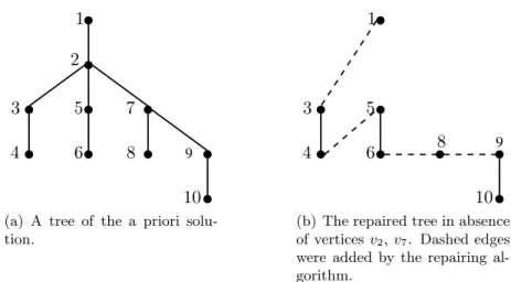
Example Fig. 1(a) depicts a tree of an a priori solution numbered according to DFS vis-itation starting from a leaf-vertex. The corresponding ordered list produced in this way is L = {1, 2, 3, 4, 2, 5, 6, 2, 7, 8, 7, 9, 10}. Assuming that vertices 2 and 7 are absent from the vertex set of the actually materialized subgraph, all occurences of these vertices are dropped from L and L" _{= {1, 3, 4, 5, 6, 8, 9, 10} emerges. The repairing agorithm scans L}" _{in order and}

adds edges (1, 3), (4, 5), (6, 8), (8, 9), so as to reconnect the remainders of the a priori tree, as shown in fig. 1(b).

We prove the following:

Proposition 1 The repairing algorithm produces a connected tree T1,l out of tree T0,l of the

9 1 2 3 4 5 6 7 8 10

(a) A tree of the a priori solu-tion. 9 1 3 4 5 6 8 10

(b) The repaired tree in absence of vertices v2, v7. Dashed edges

were added by the repairing al-gorithm.

Figure 1: Functionality of the repairing algorithm over a particular tree of an a priori forest. Proof. For every vertex vj in L" there is an appearance of vj in L" after a vertex vi with

i < j, so that vj is connected to vi by the end of the repairing algorithm. This holds for all

vertices, apart from the one appearing first in L"_{. This implies that all vertices are connected}

into one component by the end of execution of the repairing algorithm for T0,l. Furthermore

the emerging construction cannot contain cycles for two reasons: T0,l did not have cycles

and in order for a cycle to occur in the repaired solution T1,l, insertion of at least one edge

(vi, vj) is required while its endpoints have been already connected. This cannot happen by

functionality of the repairing algorithm. ! Since the repairing algorithm reconnects on G1 every single tree of the a priori solution

that was disconnected, the union of all such repaired trees along with trees that survived unaffected on G1 yields a feasible Steiner Forest on G1. These trees remain pairwise

vertex-disjoint as they were in the a priori solution, because the repairing algorithm uses only edges to reconnect trees and no such edge connects vertices belonging in different trees. Thus f0= f1 is guaranteed.

The complexity of the repairing algorithm is almost linear in the number of vertices of G0. Indeed, a DFS over a tree T0,l is of O(|T0,l|) time, while by using UNION-FIND

disjoint sets representation for maintaining connected components during the scan of L"_{, an}

O(_|T0,l|α(|T0,l|)) time is spent. Summing over all trees of the a priori forest F0, and because

|T0,l| = O(n), we obtain O(nα(n)) total time for producing the final feasible forest F1.

Theorem 1 Given an arbitrary feasible a priori solution F0, the expected cost of a repaired

solution F1 is: E[c(F1)] = f1 ! l=1 " ! (vi,vj)∈T0,l pipjc(vi, vj) + ! (vi,vj)∈E(V (T0,l))\T0,l c(vi, vj)pipj× # vl∈[vi,vj ]Ll : i<j ,_{vi,vj "∈[vi,vj ]Ll}

(1 − pl)

$

where V (T0,l) is the set of vertices incident to edges of T0,l, and E(V (T0,l)) is the set of all

edges induced by vertices in V (T0,l). Furthermore, Ll is the ordered list for tree T0,l and

[vi, vj]Ll the sublist of Ll starting at vi and ending in vj not including these two vertices. For

Proof. Each individual expression summed for tree T0,l consists of two terms, the first

one expressing the expected cost of surviving edges in the materialized subgraph (that is the expected cost of T"

0,l), while the second expresses the expected cost of edges added to T0,l" by

the repairing algorithm, so that T"

0,l is augmented into a feasible tree T1,l. The first term is

justified by the fact that (vi, vj) ∈ T0,lsurvives in T0,l" if and only if both its endpoints survive.

This happens with probability pipj, since these two events are independent.

The second term emerges by inspection of the functionality of the repairing algorithm. When G1materializes, missing vertices (in V0\V1) are dropped from the ordered list encoding

Ll and the modified list L"l emerges. The repairing algorithm scans L"l and for every pair of

consecutive vertices vi, vj it connects them using an edge (vi, vj) if and only if i < j and vi

is not connected to vj already.

Vertices vi, vj ∈ L both survive in L"l with probability pipj. Vertices vi and vj are not

connected to each other if all vertices between vi and vj in Ll are missing from L"_l, and this

happens with probability %_{vl∈[vi,vj]L}(1 − pl). Furthermore, neither vi nor vj should appear as

intermediates in the sublist [vi, vj]Ll, otherwise they should also be missing, and would not

be encountered by the repairing algorithm. Finally, the sublist [vi, vj]Ll should not be empty,

otherwise a surviving edge (vi, vj) is implied, rendering vj connected to vi. !

Clearly the expression given in theorem 1 is computable in polynomial-time. Thus:

Corrolary 1 The problem of a priori optimizing the steiner forest problem on stochastic metric graphs, for the proposed repairing algorithm, belongs to the class NP O.

The problem is NP -hard: setting all survival probabilities of vertices of G0equal to 1, yields a

deterministic steiner forest instance. Results of section 3 imply existence of a polynomial-time 4-approximation algorithm for a priori optimization of the expression of theorem 1.

3

Approximation

In this section we carry out appropriate analysis so as to show that the Steiner Forest problem over a stochastic metric graph can be approximated efficiently within a constant factor, by the repairing algorithm. The heart of our results is the following theorem:

Theorem 2 If F1 is a repaired feasible solution produced by the proposed repairing algorithm

for the Steiner Forest problem on a stochastic metric graph, given an a priori feasible solution F0, then c(F1) ≤ 2c(F0).

The proof of this result is carried out by an analysis of the algorithm over each tree T0,l

separately. The result emerges by summing over the trees of F1. In the following we denote

by Tr,l the subset of edges added by the repairing algorithm to T0,l" . We prove first some

lemmas that will be combined towards the proof of the theorem.

Lemma 1 For every edge (vi, vj) ∈ Tr,l we have c(vi, vj) ≤ c([vi. . . vj]T0,l).

Proof. Immediate by the triangle inequality holding for the cost function c : E0 → ++. !

According to lemma 1 we can express the cost of the repaired tree T1,l as follows:

c(T1,l) = c(T0,l" ) + c(Tr,l) ≤ ! e∈T" c(e) + ! (vi,vj)∈Tr,l c([vi. . . vj]T0,l) (1)

vi vj vs vt vi vj vs vt vi vj vs vt

Figure 2: Three cases that may happen for edge (vs, vt) with respect to vi, vj (proof of

lemma 2).

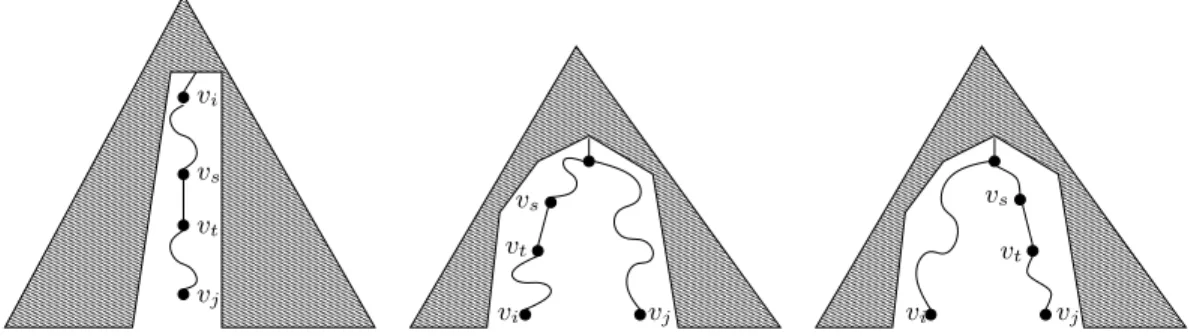
Lemma 2 For every three distinct edges (vi, vj), (vk, vl), (vq, vr) in Tr,lthe paths [vi· · · vj]T0,l,

[vk· · · vl]T0,l, [vq· · · vr]T0,l, do not share an edge in common.

Proof. By functionality of the repairing algorithm we have that i < j, k < l, q < r. Furthermore, if we assume without loss of generality that the vertex pairs were encountered in the order "i, j#, "k, l#, "q, r# during scanning of L"_{, then we deduce that j < l < r. If}

the paths intersect in some common edge (vs, vt), then it must be s, t ≤ j (fig. 2 depicts all

possible cases), thus s, t < l and s, t < r. In this case edge (vs, vt) must have been scanned

at least three times during DFS: once before visitation of each of the vertices vj, vl, vr. But

this contradicts the fact that a DFS scans each edge of a graph exactly twice. ! The following lemma will help us to complete the proof of the theorem:

Lemma 3 Consider two edges (vi, vj), (vk, vl) in Tr,l. For every edge (vs, vt) with (vs, vt) ∈

[vi· · · vj]T0,l ∩ [vk· · · vl]T0,l it holds (vs, vt) -∈ T0,l" .

Proof. The proof is by contradiction. Suppose that (vs, vt) ∈ [vi· · · vj]T0,l∩ [vk· · · vl]T0,l and

(vs, vt) ∈ T0,l" . Without loss of generality we assume that the repairing algorithm encountered

first the pair "vi, vj# and afterwards the pair "vk, vl# in L". It must be i < j, k < l and j < l

(vj may coincide with vk). Since (vs, vt) ∈ [vi· · · vj]T0,l ∩ [vk· · · vl]T0,l, then we must have

s, t≤ j and, consequently, s, t < l. Furthermore, it must hold either that (i) s, t > k or that (ii) s, t > i, otherwise it should be s, t < i and, given that s, t ≤ j also, we would deduce that (vs, vt) would have been scanned twice during DFS, once before visitation of vi and once

before visitation of vj. In this case it could not have been scanned again right before visitation

of vl. Now (i) cannot hold because k ≥ j and s, t < j. If (ii) holds, i.e. s, t > i, it is implied

that the repairing algorithm did not encounter in L" _{vertices v}

k, vl and vi, vj consecutively

(fig. 3), which is a contradiction. !

The proof of theorem 2 can now be completed as follows: Proof. Relation (1) can be written:

c(T1,l) ≤ ! e∈T" 0,l c(e) + ! (vi,vj)∈Tr,l c([vi. . . vj]T0,l) = ! e∈T" 0,l c(e) + ! (vi,vj)∈Tr,l ! e∈[vi...vj]_T0,l c(e)_⇒ c(T1,l) ≤ ! e∈T" 0,l c(e) + ! (vi,vj)∈Tr,l " ! e∈[vi...vj]_T0,l:e∈T0,l" c(e) + ! e∈[vi...vj]_T0,l:e$∈T0,l" c(e)$ (2)

vi vj vs vt vk vl

Figure 3: Case s, t > i examined in the proof of lemma 3: (vs, vt) ∈ [vi· · · vj]T0,l∩ [vk· · · vl]T0,l

and suppose that (vs, vt) ∈ T0,l" . Then obviously vs, vt survive in L" and appear as

interme-diates in the two pairs "vi, vj# and "vk, vl#.

By lemmas 2 and 3 the following are implied:

! (vi,vj)∈Tr,l ! e∈[vi...vj]_T0,l:e∈T_0,l" c(e)≤ ! e∈T" 0,l c(e) (3) ! (vi,vj)∈Tr,l ! e∈[vi...vj]_T0,l:e$∈T_0,l" c(e)_{≤ 2} ! e∈T0,l\T_0,l" c(e) (4)

By replacing the relations (3) and (4) in the expression (2) we obtain: c(T1,l) ≤ 2 ! e∈T" 0,l c(e) + 2 ! e∈T0,l\T0,l" c(e)_{≤ 2c(T}0,l) (5)

Summing over all trees, since f0 = f1, we obtain that c(F1) ≤ 2c(F0). !

Now we can state our main approximation result:

Theorem 3 There is an almost linear time repairing algorithm for Steiner Forest problem on stochastic metric graphs that, when applied to an α-approximate a priori feasible solution, produces feasible solutions that are 2α-approximate to the optimum expected cost.

Proof. By theorem 2 c(F1) ≤ 2c(F0). Let OP T (G0) and OP T (G1) be the costs of an

optimum Steiner forest on G0 and G1 respectively for the given source-destination pairs, and

c(F0) ≤ αOP T (G0). It is OP T (G0) ≤ OP T (G1) for every possible subgraph G1 of G0,

because every feasible solution for G1 is also feasible for G0. Thus c(F1) ≤ 2αOP T (G1).

Taking expectation over all possible subgraphs G1 yields E[c(F1)] ≤ 2αE[OP T (G1)]. !

Corrolary 2 There is an O(nα(n)) time repairing algorithm for the Steiner Forest problem on stochastic metric graphs, that can be supported by a polynomial-time algorithm for taking a priori decisions [1, 8], so as to yield factor 4 approximation of the optimum expected cost. The repairing algorithm is 2-approximate given an a priori optimum feasible solution. We note that in both cases mentioned in the corollary, the proposed repairing algorithm is faster than the algorithm used for a priori decisions, and is far more efficient than the trivial practices discussed in the introduction: in fact, any approximation algorithm used for taking a priori decisions (including the one of [1, 8]) will incur Ω(n2_{) complexity.}

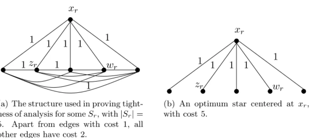
xr zr w_r 1 1 1 1 1 1 1 1

(a) The structure used in proving tight-ness of analysis for some Sr, with|Sr| =

5. Apart from edges with cost 1, all other edges have cost 2.

xr zr wr 1 1 1 1 1

(b) An optimum star centered at xr,

with cost 5.

Figure 4: Illustration of worst-case construction for showing tightness of analysis.

4

Tightness of Analysis

We show in this paragraph that the analysis of the repairing algorithm is tight for arbitrary a priori solution F0. We construct a worst-case example.

We consider a metric graph G0(V0, E0). For some fixed constant k take k sets of vertices

S1, . . . , Sk, along with a vertex xr -∈ Sr, r = 1 . . . k, per subset. Let the input metric graph

consist of the vertex set V0 = "

∪k r=1Sr

$

∪ {xr|r = 1 . . . k}. We take |Sr| = n so that

|V0| = Θ(n), because k is a fixed constant. We set c(xr, y) = 1 for each y ∈ Sr, r = 1 . . . k.

For each Sr pick two distinct arbitrary vertices wr, zr ∈ Sr and set c(zr, y) = 1 for all

y _{∈ S}r\ {wr, zr} and c(zr, wr) = 2. For all other edges of the graph we set their cost equal to

2. Fig. 4(a) shows the construction for a particular set Sr.

The Steiner Forest instance that we consider requires that each Sris connected (it is trivial

to express this requirement with source-destination pairs). We assume that the stochastic graph is defined by setting the survival probability of each xr equal to p. An optimum a

priori solution to this instance is defined as a forest consisting of an optimum connecting tree per vertex set Sr. We consider such an a priori solution that the corresponding tree for Sr is

the star Tr = {(x, y)|y ∈ Sr}. Fig. 4(b) shows the construction for a particular vertex set Sr

and the optimum star tree solution for this set.

Among the various cases that may occur in the actually materialized subgraph of G0 we

consider the one where all vertices xr, r = 1 . . . k survive, and the case where all vertices

xr are missing. For the first case the a priori optimum solution remains feasible and has an

optimum cost of &k

r=1|Sr|, while in the second case, the repairing algorithm is executed for

each tree Tr. Fig. 5 depicts the DFS numbering of a tree Tr by the repairing algorithm, and

the corresponding repaired solution. It is easy to see that such a “chain” as the one appearing in fig. 5(b), must have a cost at least 2(|Sr| − 1) − 2 = 2(|Sr| − 2), because in this chain zr

may be incident to two vertices that are connected with two edges of cost 1 to it. However, the optimum cost for the materialized subgraph occurs if we connect per set Sr its vertices to

zr, and is equal to |Sr|. Clearly the optimum expected cost is at most &kr=1|Sr| = k(n − 1),

while the solution produced by the repairing algorithm has an expected cost of value at least pk&k

r=1|Sr| + 2(1 − pk)&kr=1(|Sr| − 2) = kpk(n − 1) + 2k(1 − pk)(n − 2). Hence, the

approximation factor is asymptotically lower-bounded by: lim_n→∞ kpk_{(n−1)+2k(1−p}k_)(n−2)

k(n−1) =

xr zr wr 1 1 1 1 1 1 2 3 4 5 6

(a) DFS numbering produced by the re-pairing algorithm for star connection of Sr. zr wr 1 1 1 3 4 5 6

(b) A feasible tree produced over a dis-connected star tree, when xris missing.

Figure 5: DFS numbering and repaired tree assumed in showing tightness of analysis.

5

Conclusions

We considered the Steiner Forest problem in stochastic metric graphs, where each vertex that is not a source or destination is present with a given probability independently of all other vertices. The problem amounts to coming up with a feasible Steiner Forest for every possible materializable subgraph of the given graph, so as to minimize the expected cost of the resulting solution taken over the distribution of these subgraphs. We designed an efficient algorithm that runs in almost linear time in the number of vertices that adjusts efficiently a priori taken decisions. Given that a priori decisions constitute a feasible forest on the original metric graph we were able to derive a polynomial time computable expression for the expected cost of a Steiner Forest produced by the proposed algorithm. Furthermore, we have shown that this algorithm at most doubles the cost of the a priori solution, and this leads to 2 approximation of the optimum expected cost given an optimum a priori solution, and 4 approximation given a 2 approximate solution. Our analysis of the proposed repairing algorithm was shown to be tight.

We note that for the more special case of the Steiner Tree problem in the same model, the well-known minimum spanning tree heuristic [18] that includes only vertices requiring connection, gives a feasible and 2-approximate a priori solution that trivially remains feasible and 2-approximate for the actually materialized subgraph. As a non-trivial aspect of future work we consider extending our results to the case of complete graphs with general cost functions. Simply using shortest-path distances on these graphs does not straightforwardly lead to efficient and approximate repairing algorithms.

References

[1] A. Agrawal, P. N. Klein, and R. Ravi. When Trees Collide: An Approximation Algo-rithm for the Generalized Steiner Problem on Networks. SIAM Journal on Computing, 24(3):440–456, 1995.

[2] D. Bertsimas. Probabilistic Combinatorial Optimization. PhD thesis, 1988.

[3] D. Bertsimas. The probabilistic minimum spanning tree problem. Networks, 20:245–275, 1990.

[4] J. R. Birge and F. Louveaux. Introduction to Stochastic Programming. Springer-Verlag New York, 1997.

[5] G. W. Dantzig. Linear programming under uncertainty. Management Science, 1:197–206, 1951.

[6] K. Dhamdhere, R. Ravi, and M. Singh. On Two-Stage Stochastic Minimum Spanning Trees. In Proceedings of the International Conference on Integer Programming and Com-binatorial Optimization (IPCO), pages 321–334, 2005.

[7] L. Fleischer, J. Koenemann, S. Leonardi, and G. Schaefer. Simple cost sharing schemes for multicommodity rent-or-buy and stochastic steiner tree. In Proceedings of the ACM Symposium on Theory of Computing (STOC), pages 663–670, 2006.

[8] M. X. Goemans and D. P. Williamson. A General Approximation Technique for Con-strained Forest Problems. SIAM Journal on Computing, 24(2):296–317, 1995.

[9] A. Gupta and M. P´al. Stochastic Steiner Trees Without a Root. In Proceedings of the International Colloquium on Automata, Languages and Programming (ICALP), pages 1051–1063, 2005.

[10] A. Gupta, M. P´al, R. Ravi, and A. Sinha. What About Wednesday? Approximation Algorithms for Multistage Stochastic Optimization. In Proceedings of the International Workshop on Approximation and Randomized Algorithms (APPROX-RANDOM), pages 86–98, 2005.

[11] A. Gupta, Martin P´al, R. Ravi, and A. Sinha. Boosted sampling: approximation algo-rithms for stochastic optimization. In Proceedings of the ACM Symposium on Theory of Computing (STOC), pages 417–426, 2004.

[12] A. Gupta, R. Ravi, and A. Sinha. An Edge in Time Saves Nine: LP Rounding Ap-proximation Algorithms for Stochastic Network Design. In Proceedings of the IEEE Symposium on Foundations of Computer Science (FOCS), pages 218–227, 2004.

[13] N. Immorlica, D. R. Karger, M. Minkoff, and V. S. Mirrokni. On the costs and benefits of procrastination: approximation algorithms for stochastic combinatorial optimization problems. In Proceedings of the ACM-SIAM Symposium on Discrete Algorithms (SODA), pages 691–700, 2004.

[14] P. Jaillet. Probabilistic Traveling Salesman Problems. PhD thesis, 1985.

[15] C. Murat and V. Th. Paschos. The probabilistic longest path problem. Networks, 33(3):207–219, 1999.

[16] C. Murat and V. Th. Paschos. A priori optimization for the probabilistic maximum independent set problem. Theoretical Computer Science, 270(1–2):561–590, 2002. [17] C. Murat and V. Th. Paschos. On the probabilistic minimum coloring and minimum

k-coloring. Discrete Applied Mathematics, 154(3):564–586, 2006.