UNIVERSITÉ DE SHERBROOKE
Faculté de Lettres et de Sciences humaines
Département de Géomatique Appliquée
ACCURACY IN STARPHOTOMETRY
Liviu Ivănescu
Thesis submitted in partial fulfilment of the requirements for the
degree of philosophiæ doctor (Ph.D.) in physics of the remote sensing
April 2020
Sherbrooke, Québec, Canada
JURY
Supervisor: Prof. Norman T. O’Neill
Internal Member: Prof. Yannick Huot
Internal Member: Adj. Prof. Martin Aubé
Sommaire
La photométrie ou spectrophotométrie stellaire, est une méthode de télédétection
passive pour mesurer l’épaisseur optique spectrale de l’atmosphère. Ceci est accompli
en comparant le signal mesuré avec le rayonnement extra-atmosphérique d’une étoile
de référence. La photométrie stellaire a été introduite au début des années 1980
[
1
,
17
], en tant que contrepartie nocturne de la photométrie solaire [
6
] afin d’obtenir
une surveillance continuelle sur 24 h de l’épaisseur optique des aérosols.
Malgré
toutes les avancées technologiques, une photométrie stellaire robuste, avec exactitude
de mesure, reste un défi [
5
,
2
], qui a limité son évolution.
L’objectif général de ce travail est de susciter la confiance et l’intérêt pour la
photométrie stellaire en améliorant sa fiabilité, son exactitude de mesure et en
iden-tifiant les cas particuliers où elle surpasse la photométrie solaire (qui est en fait
une photométrie stellaire dont l’étoile est notre Soleil). Pour atteindre cet objectif,
nous devons mieux comprendre, en détails, la nature des attributs spécifiques de la
photométrie stellaire: les différentes classes spectrales des étoiles, les propriétés des
sources de référence plus faibles, les conséquences d’une plus grande ouverture de
télescope, un champ de vision (en anglais, Field Of View - FOV) moindre etc.
L’amélioration de la fiabilité de la photométrie stellaire (qui est ultimement
as-sociée à son taux de collecte de données) devrait être abordée à la fois par des
améliorations matérielles, ainsi que par des meilleures stratégies d’observation pour
atténuer les défis environnementaux. L’exactitude de mesure de l’épaisseur optique
reste critique pour certaines méthodes d’extraction de caractéristiques de
partic-ules, qui nécessitent une erreur d’épaisseur optique inférieure à 0.01 [
14
], ou une
erreur photométrique équivalente de 1%. Bien qu’une telle cible soit généralement
atteinte en photométrie solaire [
18
], elle représente toujours un défi en photométrie
Sommaire
stellaire. Afin de répondre à une telle exigence d’exactitude, il est essentiel d’identifier
toutes les principales sources d’erreurs, de faciliter la quantification de l’exactitude
et, éventuellement, d’atténuer les divers mécanismes d’erreur.
Un avantage clé de la photométrie stellaire, en plus de fournir des observations
noc-turnes en complément à la photométrie solaire, est son efficacité d’observation de 100%
en présence de ciel clair. En revanche, l’autre alternative d’observation nocturne, la
photométrie lunaire [
4
], est limitée à une efficacité de 50% (soit, entre le premier et
le dernier quart de lune). La photométrie stellaire est particulièrement pertinente
près des pôles, pendant la longue nuit polaire. Elle permet des mesures scientifiques
à partir d’une région et durant une période pour laquelle on dispose généralement de
très peu d’informations. A part cela, la disponibilité de nombreuses sources stellaires
garantit l’acquisition d’observations dans presque toutes les directions. Cela facilite
l’acquisition synergétique de données provenant d’autres instruments: les exemples
clés incluent les lidars terrestres (généralement orientés vers zénith) ([
8
], les lidars
satellitaires, tels que CALIOP pointant vers nadir, à bord du satellite CALIPSO
[
11
] et le lidar Doppler ALADIN à pointage oblique, à bord de l’ADM-Aeolus [
7
]. De
plus, étant donné que la diffusion frontale dans le cas des FOV larges des photomètres
solaires et des photomètres lunaires peut induire une sous-estimation importante de
l’épaisseur optique [
12
], les FOV significativement moindre des photomètres stellaires
garantissent un avantage distinct de la photométrie stellaire à cet égard.
Un aspect important de l’objectif du projet est d’identifier et quantifier des sources
inconnues d’erreurs d’exactitude. Un attribut particulièrement frustrant de la
pho-tométrie stellaire est que même les erreurs connues sont difficiles à estimer.
En
fait, même si elles sont estimées par comparaison avec d’autres instruments (lidars,
d’autres photomètres stellaires ou lunaires), ces erreurs peuvent également varier en
fonction de différentes conditions d’observation. Le niveau de confiance dans ces
sys-tèmes reste par conséquent faible. Si l’utilisation de masse est un avantage pour la
maturation des instruments, alors la photométrie stellaire est désavantagée: il n’y a
actuellement que 2–3 photomètres stellaires opérationnels dans le monde. En outre,
le degré plus élevé de complexité technique et le taux de panne par rapport aux
pho-tomètres solaires et lunaires, leurs exigences élevées en matière de maintenance et de
dépannage, peuvent les rendre peu attrayants pour les observatoires opérationnels.
Sommaire
En raison de la faible demande de photomètres stellaires qui en résulte, Dr. Schulz
& Partner GmbH (la seule entreprise fabriquant des photomètres stellaires en série)
a cessé ses activités avant de pouvoir résoudre correctement certains des problèmes
techniques identifiés par les utilisateurs (par exemple, surchauffe interne, revêtement
antireflet inapproprié de lentilles, accès indisponible à certains paramètres critiques
etc.). Cela conduit à un cycle de méfiance: il faut de nombreuses observations et
études pour améliorer la fiabilité et l’exactitude, alors que nous n’avons pas assez
d’instruments opérationnels en raison de leurs problèmes techniques et de leur
exac-titude discutable.
Les photomètres stellaires ont également leur lot de défis spécifiques reliés au site
d’observation. Un problème courant est le dépôt de poussière, de rosée, de givre ou de
particules de glace sur le télescope (avec des effets associés sur l’atténuation optique).
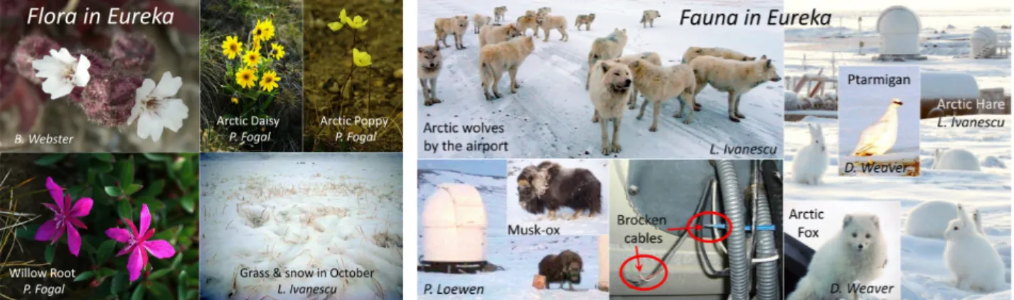
Un site polaire, comme Eureka, pose plusieurs défis supplémentaires: turbulence de
l’air plus élevée près du niveau de la mer (avec des effets sur la taille de l’image
de l’étoile), scintillation plus élevée à grande masse d’air (affectant la précision de
la mesure), température ambiante très basse (affectant le matériel, notamment les
pièces mécaniques en mouvement et le câblage électrique), le pergélisol (empêchant
une bonne mise à la terre électrique), le bien-être des instruments à proximité
(sensi-bles aux interférences électromagnétiques, ou EMI), l’emplacement en région éloignée
(ce qui signifie de longs retards dans l’expédition des pièces pour les réparations), air
très sec (dégazage de composants électroniques), assistance limitée sur le site (pour
l’opération et la maintenance), accessibilité dangereuse (environnement non-protégé
contre les animaux sauvages: loups, bœufs musqués, ours polaires), internet très lent
(pour le transfert de données ou l’opération à distance). Nos photomètres stellaires
ont subi plusieurs pannes matérielles, chaque année au cours de leurs 11 années de
fonctionnement. Cela a entraîné un risque élevé de ne pas pouvoir terminer les études
prévues en temps opportun. Nous décrivons ici nos contributions techniques et
sci-entifiques issues du projet de thèse.
Article
1
: Bien que cet article initial ait été rigoureusement examiné en vue de
publication par le comité des SPIE Proceedings, il n’était néanmoins pas ciblé comme
un article scientifique évalué par les pairs, mais plutôt comme une introduction à
la photométrie stellaire arctique et à ses défis techniques.
Il décrit en détail les
Sommaire
développements que nous avons faits pour surmonter les principaux problèmes
tech-niques et logistiques liés à l’exploitation d’un photomètre stellaire dans un endroit
éloigné et à environnement hostile, tel qu’Eureka. Réussir dans ce cas extrême
pour-rait, espérons-le, fournir la confiance nécessaire dans la fiabilité de la photométrie
stellaire. Ces travaux ont notamment identifié: les problèmes de mise à la terre
élec-trique dus au pergélisol, le dégazage dû à l’air sec, les problèmes de débit optique
dus au revêtement des lentilles, le problème majeur du dépôt de cristaux omniprésent
sur le télescope et la nécessité d’une opération à distance. Pour plus d’informations,
l’article est présenté au Chapitre
1
.
Article
2
: Le deuxième article est le principal travail scientifique de télédétection
de la thèse, dans la mesure où ils partagent le même titre. Dans le Chapitre
2
,
il développe en détail le cadre théorique de la photométrie stellaire, conduisant à
l’identification de tous les paramètres susceptibles d’induire des erreurs importantes.
Il identifie en particulier l’avantage d’effectuer un étalonnage indépendant de l’étoile,
mais néanmoins dépendant de l’instrument. Ensuite, il explore en profondeur et,
espérons-le, identifie les principales sources d’erreurs d’exactitude spécifiques à la
photométrie stellaire et fournit des solutions d’atténuation. Une investigation aussi
approfondie, particulièrement impliquant un site éloigné de l’Arctique, nécessitait
beaucoup de ressources matérielles et intellectuelles. Bien que j’aie effectué tout le
travail décrit dans l’article, au-delà des précieuses contributions de mes collègues
coauteurs, les conseils constants, les contre-vérifications scientifiques rigoureuses et la
vérification approfondie du texte par mon superviseur ont été déterminants. Enfin, la
disponibilité constante pour assurer la maintenance, par les fabricants du photomètre
stellaire, du dôme et de la monture de télescope, a été primordiale.
Article
3
: Alors que nous travaillons simultanément sur une analyse complète des
procédures d’étalonnage, la courte communication présentée au Chapitre
3
vise à
at-teindre plus rapidement la communauté scientifique en soulignant qu’un étalonnage
multi-étoiles, indépendant d’étoile, peut être effectué sur place, même près du niveau
de la mer. On y commence par présenter statistiquement les périodes de ciel clair
typiques pour Eureka. Ensuite, on souligne la rapidité de l’étalonnage multi-étoiles,
évitant des variations importantes de transparence du ciel et lissant certaines des
inexactitudes du catalogue extra-atmosphérique de magnitudes d’étoiles. La
Sommaire
bilité d’un tel étalonnage multi-étoiles n’apparaît qu’à la suite de l’accent mis sur
l’utilisation d’un étalonnage indépendant d’étoile dans l’article
2
. De plus, il est
démontré qu’une méthode d’étalonnage particulière, appelée « inverse », réduit
da-vantage les erreurs d’étalonnage, approchant notre cible d’exactitude. Cet objectif
principal est confirmé par une analyse de répétabilité.
Bien que d’importants développements en photométrie stellaire aient été réalisés
au cours de la dernière décennie, principalement par Perez-Ramirez [
16
,
15
], une
anal-yse complète des erreurs d’exactitude n’a pas été effectuée depuis les travaux de Young
[
19
] dans les années 1970, dans le contexte de l’astronomie professionnelle. Notre
tra-vail le met à jour et le complète avec la réalité technologique actuelle et la spécificité
de la photométrie stellaire pour la télédétection atmosphérique. Cela nous a permis
d’évaluer quantitativement les principales sources d’erreurs et de songer comment y
remédier. Parmi nos trouvailles originales sont les lignes gênantes d’absorption d’O
4,
jusqu’à présent non considérées dans le contexte de la photométrie stellaire. Elles
em-pêchent une élimination exacte de la bande d’ozone, conduisant à une distorsion du
spectre d’aérosol déduit. Nous avons identifié un FOV de 45
00, optimisé pour une
util-isation en photométrie stellaire, comme compromis pour préserver le débit optique,
ainsi que limiter les erreurs de diffusion frontale lors de l’observation des nuages. On
a également identifié pour la première fois l’avantage de la photométrie stellaire par
rapport à la photométrie solaire dans un tel contexte. Nous avons souligné pour la
première fois l’importance de l’utilisation de classes spectrales des étoiles froides (par
exemple, la classe F) lors de l’observation des nuages, et généralement l’utilisation des
étoiles B précoces ou A tardives quand une meilleure exactitude est requise. Le dépôt
de cristaux sur la fenêtre d’entrée du télescope dans l’Arctique a longtemps semblé
être un gros et insurmontable problème. Après plusieurs essais, nous avons identifié
l’utilisation d’une bande chauffante autour du télescope, en tant que solution efficace
dans la plupart des situations environnementales. Toutes ces améliorations suggèrent
que l’atteinte de la cible d’exactitude de 1% pourrait devenir enfin possible. De plus,
notre mise en œuvre de l’opération et de la maintenance à distance, pouvant être
effectuée même à partir d’un téléphone intelligent, c’est-à-dire à tout moment et de
n’importe où dans le monde, est unique au moins dans la communauté de photométrie
stellaire. Cela ouvre enfin, pour la première fois, la possibilité de gagner la confiance
Sommaire
dans ce type d’instruments.
Une telle analyse approfondie aurait plutôt dû être élaborée par des efforts
con-certés de la communauté scientifique, sur plusieurs sites. La disponibilité limitée de
photomètres stellaires opérationnels et la nécessité aiguë de briser le cercle de
méfi-ance nous ont amenés à y faire face dans toute sa complexité. Cependant, le fait que
nous ayons principalement basé notre analyse sur un seul type de photomètres
stel-laires et principalement sur la spécificité d’un seul observatoire au niveau de la mer
en Arctique, peut conduire à passer à côté de certaines sources potentielles d’erreurs
spécifiques à d’autres sites. On peut supposer, par exemple, des problèmes liés à
l’humidité dans les tropiques, le dépôt de poussière dans les environnements arides
ou l’estimation erronée de la brillance de fond de ciel dans les sites fortement pollués
par la lumière, comme les villes. Au-delà de celles-ci, il est également possible que
nous ayons négligé certaines erreurs importantes, car nous avons continuellement,
et parfois de manière inattendue dans des situations spécifiques, révélé leur grande
ampleur. Nous recommandons alors que, pour valider les résultats identifiés ici, on
devrait régulièrement participer à des campagnes d’observation sur d’autres sites et
comparer l’exactitude attendue avec d’autres instruments colocalisés.
En plus de ce travail, nous sommes également très avancés dans la finalisation
d’une analyse complète des erreurs de photométrie stellaire non systématiques, de
précision. Ces résultats servent ensuite à développer une analyse complète des
méth-odes d’étalonnage (ultimement, affectant l’exactitude aussi), qui est également à un
niveau avancé de développement. Nous construisons actuellement un nouveau
cat-alogue spectrophotométrique extra-atmosphérique d’étoiles, basé sur les mesures du
satellite GOMOS, qui est essentiellement un photomètre stellaire spatial. De plus,
nous essayons de construire un modèle de luminosité du ciel, basé sur les positions
du soleil et de la lune, de l’épaisseur optique atmosphérique et des mesures de fond
de ciel du photomètre stellaire. De manière inattendue, cela semble conduire à une
autre façon de mesurer l’épaisseur optique dans des conditions de ciel brillant, offrant
un moyen de quantifier toute dégradation du débit optique du photomètre stellaire,
par exemple en raison du dépôt de cristaux.
Mots-clés: photométrie stellaire, justesse de mesure, étalonnage, aérosols, Arctique.
Acknowledgments
Since the start of my PhD project, several unforeseen challenges appeared:
contin-uous hardware failures, starphotometer manufacturer closing business, main funding
sources not being extended, hostile environments and, not less important, a new
baby. However, the support of my supervisor, Norm O’Neill, remained unshakeable.
He didn’t hesitate to get deeply involved in a humongous effort of analysing every
single bit of my results. He also knows how to build and maintain student confidence
and motivation, by continuously giving credit for the smallest achievement. Actually,
we appeared to be in a colleague-colleague, rather than a professor-student
relation-ship. Looking back, I would say that a good scientific supervisor should share a lot
with a tennis coach, sport that both of us enjoy watching: hard worker and fine
psy-chologist. In addition, I was lucky enough to have not only one good supervisor, but
unofficially two, since my MSc supervisor, Jean-Pierre Blanchet, was always ready
to help, scientifically, logistically, and even financially. I’m grateful to both of them
for their support, for believing in me and for always encouraging me to create and
develop new ideas.
Finishing up this PhD project from the family perspective looked like a far fetched
endeavour, while other down to Earth family needs have to be fulfilled with priority.
Obviously, this would have not been even possible to start without the unconditional
support of my wife Letit
,ia - my friend, my confidant and my love. I’m grateful to her
and I consider it to be a truly family project. Lastly, it would have been the honour
of my life to invite my parents to my PhD defence. For such an accomplishment my
father would have been overjoyed and my mother would have mention it for years.
Unfortunately they left us too soon for a better world. I miss them very much and
I’m grateful to them for what I am today.
to my beloved wife, Letit
,ia
Contents
Sommaire
i
Acknowledgments
vii
Contents
ix
Framework
1
0.1
Starphotometry
. . . .
1
0.2
Observing challenges
. . . .
2
0.3
Data collection
. . . .
3
0.4
Main results
. . . .
5
0.4.1
Article 1
. . . .
5
0.4.2
Article 2
. . . .
6
0.4.3
Article 3
. . . .
8
0.5
Originality
. . . .
8
0.6
Conclusion
. . . .
9
0.7
Other published work
. . . .
10
1
Challenges in operating an Arctic telescope
12
2
Accuracy in starphotometry
34
3
Multi-star calibration in starphotometry
67
Framework
0.1
Starphotometry
Starphotometry, or stellar spectrophotometry, is a passive remote sensing method
for retrieving the spectral optical depth of the atmosphere. This is accomplished by
comparing the measured signal with the extra-atmospheric radiance of a reference
star. Starphotometry was introduced in the early 1980’s [
1
,
17
] as a night
counter-part to sunphotometry [
6
] in order to obtain continuous 24 h aerosol optical depth
monitoring coverage. Despite all the technological advances, robust and accurate
starphotometry remains a challenge [
5
,
2
] that has limited its evolution.
The general objective in this work is to inspire trust and interest in starphotometry
by improving its reliability, its measurement accuracy and by identifying particular
cases where it outperforms sunphotometry (which is in fact starphotometry with
the star being our Sun). In order to achieve such an objective we need to better
understand the detailed nature of specific starphotometry attributes: the different
spectral classes of stars, the properties of weaker reference sources, the consequences
of a larger telescope aperture, a smaller Field of View (FOV) etc.
Improving starphotometry reliability (which is associated with its data collection
rate) should be addressed through both, hardware improvements and better observing
strategies for mitigating environmental challenges. The accuracy of optical depth
retrieval remains critical for particle feature extraction methods which require sub
0.01 optical depth error [
14
], or equivalently, 1% photometric accuracy. While this
target is generally achieved in sunphotometry [
18
], it still represents a challenge in
starphotometry. In order to fulfill such an accuracy requirement, it is essential to
identify all the major sources of errors, facilitate the quantification of measurement
0.2. Observing challenges
accuracy and, eventually, mitigate the diverse error mechanisms.
One key advantage of starphotometry, aside from providing nighttime observations
to complement sunphotometry, is its 100% duty cycle in the presence of clear skies.
In contrast, the other nighttime alternative, moonphotometry [
4
], is limited to a 50%
duty cycle, (i.e. between the first and last quarters of the moon). Starphotometry is
particularly relevant near the poles, during the long polar night. It enables remote
sensing measurements from a region and period for which one generally has very
lit-tle information. Beyond that, the availability of numerous stellar sources ensures the
acquisition of observations in almost any direction. This facilitates the synergistic
acquisition of data from other instruments: key examples include (generally
zenith-pointing) ground-based lidars ([
8
], satellite-based lidars, such as the nadir-pointing
CALIOP onboard the CALIPSO satellite [
11
] and the slant-path-looking ALADIN
Doppler lidar onboard ADM-Aeolus [
7
]. In addition, because forward scattering into
the broad FOVs of sunphotometers and moonphotometers can induce significant
op-tical depth underestimation [
12
], the much smaller FOVs of starphotometers ensure
a distinct advantage of starphotometry in this regard.
0.2
Observing challenges
An important aspect of the project was to identify and quantify unknown sources
of accuracy errors. A particularly frustrating attribute of starphotometry is that
even the known error types are difficult to estimate. Even if assessed by comparison
with other instruments (lidars, other starphotometers, moonphotometers), those
er-rors may also vary as a function of different observing conditions. The level of trust
in such systems consequently remains low. If mass usage is a benefit to instrument
maturation then starphotometry is at a disadvantage : there are currently only 2–3
operational starphotometers worldwide. In addition, the higher degree of technical
complexity and failure rate relative to sunphotometers and moonphotometers, their
high maintenance and troubleshooting requirements, can make them unattractive for
operational observatories. As a consequence of the attendant low demand for
starpho-tometers, Dr. Schulz & Partner GmbH (the only company fabricating
starphotome-ters as a serial product) went out of business before being able to properly fix some
0.3. Data collection
of the technical issues identified by current users (e.g. internal overheating,
inappro-priate lens coating, missing access to some critical parameters etc). This leads to a
cycle of mistrust: one needs many observations and studies to improve reliability and
accuracy, while we don’t have enough operational instruments due to their technical
issues and their debatable accuracy.
Starphotometers also have their share of specific challenges related to the observing
site. One common problem is the deposition of dust, dew, frost, or ice particles on
the telescope (with attendant effects on its optical throughput). A polar site, such as
Eureka, poses several additional challenges: greater near sea-level air turbulence (with
effects on the star spot size), higher scintillation induced variations at large airmasses
(affecting the measurement precision), very low ambient temperature (affecting the
hardware, notably the mechanical moving parts and electrical wiring), permafrost
(preventing a good electrical grounding), the impact on nearby instruments (sensitive
to electromagnetic interference, or EMI), the remote location (meaning long delays
in shipping of parts for repairs), very dry air (outgassing of electronic components),
limited on-site support (for operation and maintenance), dangerous accessibility (open
surroundings with risks of frostbite and extreme wind chill, not mention the dangers
of wild animals: wolves, muskoxen, polar bears), very slow internet (for data transfer
or remote control). Our starphotometers have undergone numerous hardware failures,
every year of their 11 years of operation. This led to a high risk of not being able to
complete the planned studies in a timely manner.
0.3
Data collection
Due to the aforementioned technical issues and challenges, data collection in
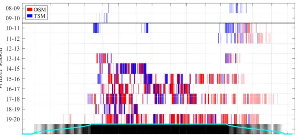
Eu-reka (our only operational site) has, as made evident in Figure
1
, sustained frequent
gaps throughout the 11 years of operation at that site. On that figure, OSM and
TSM represent One-Star Measurement and Two-Star Measurement operating modes,
respectively. The OSM mode is principally used under cloudy skies to capture their
higher temporal optical depth variability or over a longer unsupervised period of clear
and/or partially cloudy conditions by observing Vega (a high star allowing more
ro-bust observations in the case of high optical depth). The TSM mode is principally
0.3. Data collection
Figure 1 – Starphotometer data collection duty cycle. OSM and TSM stand for
One-Star Measurement (red vertical bars) and Two-Star Measurement (blue vertical
bars) operating modes, respectively. The width of the black vertical bars represent
the nighttime duration from sunset to sunrise (they merge into a single black mass
during the polar night), while the height of the cyan curve is indicative of nighttime
duration (see text for details on the nighttime duration).
used in clear sky conditions (for calibration check), or during aerosol events. The
bottom dark bands of Figure
1
represent the nighttime from sunset to sunrise, i.e. up
to 50
0below the horizon (a number that accounts for the refractive bending of the
solar disk). The height of thee cyan curve represents the nighttime duration where
the end of the night is marked by the sun being 6
◦below the horizon rather than the
refractive horizon (6
◦below the horizon being the start of the civil twilight period
for which one generally cannot make observations). More details on the observation
modes are presented in the second article of the thesis.
The first two winter measurement seasons (2008-2010), during which we worked
with older versions of the starphotometer and mount/dome, were carried out on a
campaign basis. This was principally because the telescope mount and dome were
not ruggedized for continuous Arctic operation, and because of the limited
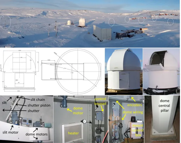
availabil-ity of supervised operation. Starting in 2010 we installed the latest starphotometer
version and a specially built dome along with a mount for Arctic conditions (see
0.4. Main results
details in the first article). During the first four winter observing seasons we had
several concurrent hardware failures and had to deal with the frustrating impact of
starphotometer EMI emissions on nearby meteor radar measurements along with the
data collection compromises that had to be implemented to temporarily sidestep the
issue. After mitigating the EMI issue by relocating the compromised meteor radar
array, the data collection rate improved. A starphotometer overheating issue, once
identified, was worked around simply by implementing another layer of protection:
an analogue thermostat that turns off the internal computer when the software-based
internal temperature control fails. In order to limit such abrupt observation
shut-downs, we also reverse engineered the main electronic control board since the original
design was no longer available (we re-designed it in India and manufactured it in
Romania). This led to a significant improvement in data collection (starting with the
2015-2016 season). Another issue occurred however in the second half of the
2016-2017 season, by the filling up of the small amount of space initially allocated to the
starphotometer operating system (the problem was fixed the following summer in an
UQAM laboratory). Another notable issue in the second half of the 2018-2019 season
was a damaged telescope-mount OS card (replaced by the manufacturer with a more
robust OS card).
0.4
Main results
Our technical and scientific contributions resulting from the PhD project are
de-scribed in the following three articles.
0.4.1
Article 1
While this initial article was refereed according to the proceedings standards of
SPIE Proceedings board, it was nevertheless not targeted as a peer reviewed
scien-tific paper, but rather as an introduction to Arctic starphotometry and its technical
challenges. It describes in detail, the challenges we had to overcome in addressing the
technical and logistical issues related to operating a star-photometer in a remote and
environmentally hostile location such as Eureka. The success that we achieved in this
0.4. Main results
extreme environment should, we hope, inspire trust in the reliability of
starphotome-try in general. In this paper we addressed a number of important problems: electrical
grounding issues due to permafrost, outgassing due to dry air, optical throughput
is-sues due to the lens coating, the major issue of the omnipresent crystal deposition on
the telescope and the necessity for remote operation. For more detailed information,
the article is presented in Chapter
1
.
0.4.2
Article 2
The second article (Chapter
2
), of the same title as this thesis, contains the
principal remote sensing research results of the PhD project. It elaborates on the
theoretical starphotometry framework and identifies the parameters susceptible to
inducing significant errors. It notably identifies the advantage of performing a star
independent (instrument dependent) calibration. Most major sources of accuracy
errors specific to starphotometry are identified and analyzed with a view to providing
mitigation avenues. A singular emphasis was placed on achieving an optical depth
error of less than 0.01. The main contributions are summarized below:
• The inaccuracies of star catalogs (absolute reference sources) was determined to
be a major problem, particularly in the case of bandwidth mismatch between the
catalog and the instrument. One way of avoiding star catalogs is to frequently
calibrate a given instrument relative to a given star (or stars) at a high altitude
observatory: this is, however, impractical due to technical challenges related
to, for example, frequent installation, de-installation and transport impacts on
instrument stability and the availability of the same stars at the home and
calibration sites. A more practical solution is to build a more accurate high
resolution spectrophotometric catalog for bright stars that would enable a star
independent calibration (a catalog whose member magnitudes would preferably
be measured from space). Such flexibility would enable on-site calibration.
• Detector spectral drift may generate major accuracy errors related to the large
slope of the stellar spectra. On-site spectral calibration can be frequently
per-formed by taking advantage of stellar and telluric (atmospheric trace gas)
ab-sorption lines.
0.4. Main results
• The spectral location of the standard starphotometer channels must avoid the
deep stellar and telluric absorption lines. This is more critical for some
spec-tral classes of stars (B4 to A6) with deeper absorption lines. In this context,
we notably identified problematic O
4telluric absorption lines and proposed an
optimised channel allocation.
• Airmass inaccuracy may become important at large airmasses, if they are
cal-culated from time stamp data, so it requires accurate GPS time recording. In
this context we demonstrated the advantage of acquiring data from a higher
altitude site.
• The forward scattering error is a major issue when observing through
semi-transparent clouds. We demonstrated that our starphotometers readily attained
the 0.01 error target with the exception of certain large-particle ice clouds. This
result underscored the distinct advantage of starphotometry over large-FOV sun
or moonphotometry.
• The high brightness and associated variability of the near infrared spectrum of
the sky background may be a limitation for accurate identification and
param-eterization of coarse mode particles such as coarse mode aerosols and clouds.
The problem may be mitigated with a colder F class star such as Procyon which
is brighter in the near infrared (the spectral class essentially being related to
the effective surface temperature of the star).
• Several issues specific to our type of starphotometers were identified and
quan-tified. These were mostly limited to optical alignment, linear detection range,
temperature control and other shortcomings that could potentially have
signif-icant impacts. In this context, we identified a minimum required FOV that
ensures the integrity of the stellar flux detection, i.e. the preservation of the
optical throughput.
• An issue of particular importance in the Arctic is the deposition of ice crystals
on the telescope. This problem significantly affects the optical throughput: it
was investigated and a mitigation solution that employed heating bands around
the telescope tube was successfully implemented.
This comprehensive investigation, involving the notable complications of a remote
7
0.5. Originality
Arctic site, necessitated the bringing to bear of considerable material and intellectual
resources. While I performed virtually all the field and lab work described in the
article, the input I received from my co-author colleagues and the constant advice,
rigorous scientific cross-checks and in-depth text proofing of my supervisor were
de-termining factors. Lastly, the constant availability of the Eureka operations staff and
the instrument manufacturers in providing maintenance assistance and advice for the
starphotometer, dome and telescope mount was paramount.
0.4.3
Article 3
While we are concomitantly working on a comprehensive analysis of the calibration
procedures, the letter presented in Chapter
3
was intended to more rapidly
commu-nicate the innovative notion that a star independent calibration may be performed
on-site (even at near sea-level elevations). The paper starts with a statistical analysis
of typical clear sky periods for Eureka. The rapidity of the multi-star calibration
and the avoidance of significant sky transparency variations is then underscored. The
possibility of such a multi-star calibration is a direct consequence of concepts
pre-sented in Article
2
on the advantages of using a star independent calibration. We
also demonstrated that a particular "Reversed" calibration method further reduced
the calibration errors to values approaching the 0.01 accuracy target of Article
2
. The
achievement of this target was confirmed by means of a repeatability analysis.
0.5
Originality
While important starphotometry advances were achieved over the last decade,
notably by Perez-Ramirez [
16
,
15
], a comprehensive analysis of accuracy errors has
not been carried out since the astronomy studies of Young [
19
] in the 1970’s. Our
work updates and complements those investigations to the current technological
re-ality and specificity of starphotometry for atmospheric remote sensing. This allowed
us to quantitatively asses the main sources of errors and how to address them. We
identified the contaminating effects of the O
4absorption lines, an artefact that has
not been reported in the starphotometry literature. These features inhibit accurate
0.6. Conclusion
ozone optical depth removal and accordingly lead to a distortion of the retrieved
aerosol spectrum. We identified an optimised 45
00FOV for use in starphotometry:
this number represented a compromise between preserving the optical throughput
and limiting the forward scattering errors when observing clouds. We also identified,
for the first time, the starphotometry advantage over sunphotometry in the context
of the forward scattering errors. Another original contribution was to promote the
importance of employing the cold star spectral class (e.g. F class) when observing
clouds and generally the use of early B stars or late A stars if better accuracy is
required. The crystal deposition on the telescope entry window seemed, for a long
time, to be an impossible issue to solve. After several trials, we found that a
heat-ing band was a successful solution for most environmental situations. All of these
above-mentioned improvements suggested that achieving the 1% accuracy mark was
finally feasible. In addition, our implementation of remote control and maintenance
procedures that could be carried out using a smart phone (i.e. anytime and from
anywhere in the world) are unique, at least in the starphotometry community. This
finally opens up, for the first time, the possibility for building trust in this type of
instruments.
0.6
Conclusion
Such comprehensive analysis should have been supported by concerted
commu-nity efforts across several sites. The limited availability of operational
starphotome-ters and the acute necessity to mitigate the level of mistrust in these instruments,
motivated our efforts to address this problem in all its complexity. However, the fact
that we based our analysis principally on only one type of starphotometer and largely
on one Arctic sea-level observatory, may have lead to the neglect of potential errors
specific to other sites: for example, humidity related issues in the tropics, dust
de-position in arid environments, or sky background biases at sites suffering from urban
light-pollution. Beyond those examples, we may still have neglected other important
errors, as we continuously, and sometimes unexpectedly, encountered large magnitude
signal anomalies in specific situations. Accordingly, in order to validate the findings
identified here, we recommend regular participation in observing campaigns at other
0.7. Other published work
sites in order to compare and validate the expected accuracy with other collocated
instruments.
In addition to this work, we are finalising a comprehensive analysis of non-systematic
starphotometry errors (errors in precision). Those results further advance our goal
of a comprehensive analysis of calibration methods (ultimately affecting the accuracy
too). We are currently generating a new extra-atmospheric spectrophotometric star
catalog, based on measurements of the GOMOS sensor, which is basically a
space-based starphotometer. In addition, we are formulating a sky brightness model that is
based on the sun and moon positions, atmospheric optical depth and starphotometer
sky background measurements. This has tentatively lead to an alternative way of
measuring the optical depth in bright background conditions and thereby, a tool for
flagging and quantifying any starphotometer optical throughput degradation (due to
crystals deposition, for example).
0.7
Other published work
1. Ivănescu L.: Une application de la photométrie stellaire à l’observation de
nuages optiquement minces à Eureka, NU, MSc thesis, UQAM, 2015* [
8
].
- Contribution: My Masters in Science (MSc) thesis in Atmospheric Sciences (*
"An application of starphotometry to the observation of optically thin clouds
in Eureka, NU") overlapped the work of the PhD project due to a seemingly
endless stream of technical difficulties. It includes an original remote sensing
method for retrieving particle size and number concentration from the synergy
of radar and lidar profiles. In addition, it helped in understanding the optical
coherency of lidar-starphotometer measurements.
I also made contributions to and have been a co-author of several other
peer-reviewed articles during my PhD work.
2. Baibakov K., N. T. O’Neill, L. Ivănescu, T. J. Duck, C. Perro, A. Herber,
K.-H. Schulz, O. Schrems: Synchronous polar winter starphotometry and lidar
measurements at a High Arctic station, Atmospheric Measurement Techniques,
vol. 8, issue 9, 3789-3809, 2015 [
3
].
0.7. Other published work
- Contribution: It was partly based on data I acquired from Eureka, for which
I partly did data processing, as well as for the Alaska campaign. Several
theo-retical developments were inspired by my MSc thesis.
3. O’Neill N. T., K. Baibakov, S. Hesaraki, L. Ivănescu, R. V. Randall, C. Perro,
J. P. Chaubey, A. Herber, T. J. Duck: Temporal and spectral cloud screening of
polar winter aerosol optical depth (AOD): impact of homogeneous and
inhomo-geneous clouds and crystal layers on climatological-scale AODs, Atmospheric
Chemistry and Physics, vol. 16, issue 19, 12753-12765, 2016 [
13
].
- Contribution: I provided the processed starphotometer data from Eureka and
helped analysing it.
4. Libois Q., C. Proulx, L. Ivănescu, L. Coursol, L. S. Pelletier, Y. Bouzid,
F. Barbero, E. Girard, J.-P. Blanchet: A microbolometer-based far infrared
radiometer to study thin ice clouds in the Arctic, Atmospheric Measurement
Techniques, vol. 9, issue 4, 1817-1832, 2016 [
10
].
- Contribution: It was based on the development of an instrument (FIRR) that
I helped characterising through measurements in the lab and in the field.
5. Libois Q., L. Ivănescu, J.-P. Blanchet, H. Schulz, H. Bozem, W. R. Leaitch,
J. Burkart, J. P. D. Abbatt, A. B. Herber, A. A. Aliabadi, É. Girard:
Air-borne observations of far-infrared upwelling radiance in the Arctic, Atmospheric
Chemistry and Physics, vol. 16, issue 24, 15689-15707, 2016 [
9
].
- Contribution: It was based on the data acquired during my participation with
the FIRR to the pan-arctic Pamarcmip 2015 Polar 5/6 AWI/NETCARE
air-borne campaign. I also did data processing and the contextual satellite analysis.
6. Ranjbar K., N. T. O’Neill, L. Ivănescu, J. S. King, P Hayes: Remote sensing
of a high-Arctic, local dust event over Lake Hazen (Ellesmere Island, Nunavut,
Canada), Atmospheric Environment Journal of Elsevier, to be submitted in
2020.
- Contribution: I did meteorological data analysis and interpretation, based on
ground weather data, and from Polar 6 measurements during Pamarcmip 2015.
Chapter 1
Challenges in operating an Arctic
telescope
Foreword
Article published on 22 July 2014 in the Proceedings of SPIE
(So-ciety of Photo-Optical Instrumentation Engineers), Ground-based
and Airborne Telescopes V!
Challenges in operating an Arctic telescope
Liviu Iv˘
anescu
a,b, Konstantin Baibakov
a, Norman T. O’Neill
a, Jean-Pierre Blanchet
b, Yann
Blanchard
a, Auromeet Saha
a, Martin Rietze
cand Karl-Heinz Schulz
da
Centre d’applications et de recherches en t´
el´
ed´
etection (CARTEL), D´
epartement de
G´
eomatique Appliqu´
ee, Universit´
e de Sherbrooke, 2500, boul. de l’Universit´
e, QC, J1K 2R1,
Sherbrooke, Canada;
b
Department of Earth and Atmospheric Sciences, Universit´
e du Qu´
ebec `
a Montr´
eal (UQ `
AM),
Case postale 8888, Succursale Centre-ville, QC, H3C 3P8, Montr´
eal, Canada;
c
Baader Planetarium GmbH, 82291, Mammendorf, Germany;
d
Dr. Schulz & Partner GmbH, Falkenberger Str. 36, 15848, Buckow, Germany
ABSTRACT
We describe our seven year experience and the specific technical and environmental challenges we had to overcome while operating a telescope in the High Arctic, at the Eureka Weather Station, during the polar winter. The facility and the solutions implemented for remote control and maintenance are presented. We also summarize the observational challenges encountered in making precise and reliable star-photometric observations at sea-level. Keywords: star-photometry, Arctic, telescope, operation, site testing, astronomy, remote sensing, atmosphere.
1. INTRODUCTION
The utilization of optical telescopes in the polar environment has been explored for several decades, particularly for astronomical observations and the remote sensing of the Earth’s atmosphere. In Antarctica, the concept of stellar observations at visible wavelengths, was declared in 1987 as being impractical1.2 After finding in 1999
that the observing conditions are actually greatly improved beyond the first tens of meters above the ground,3
the quest for astronomy in Antarctica gained a new momentum.4 Aiming at more ambitious facilities on top
of 20-30 m towers,5 small optical telescopes are currently providing6 some insight into operational challenges
particular to Antarctica.7
The Arctic was perceived as being less amenable to astronomical observations, based mainly on Low Arctic (< 75◦N) Inuit knowledge,8 or the weather reports of summertime ships.9 Starting in 1993, the first sea-level,
wintertime, visible starlight observations, were in fact dedicated to atmospheric remote sensing10.11 Assessments
of the Arctic as being also appropriate for astronomy came only after 20021213,14based on satellite or radiosonde
data. Site testing in the High Canadian Arctic, based on ground observations, confirmed its excellent potential15
at high elevations.16
Optical stellar observations at ice-level in Antarctica, or at sea-level in the Arctic, are especially difficult. Drawbacks of particular note are the air turbulence and the almost omnipresent ice crystals. In spite of these factors, there is a strong scientific motivation for the investigation of low altitude atmospheric constituents, such as the low to mid-tropospheric aerosols of the Arctic haze. We report the challenges encountered in operating a sea-level optical telescope in the High Arctic, at the Eureka Weather Station (80◦N, 86◦W). The objective of this instrument was to perform accurate star pointing and photometry for remote sensing applications. A similar facility is located in Ny-Alesund, Spitsbergen (79◦N, 12◦E),17 while a third site, planned for Dome C in
Antarctica, is currently on hold.7 The challenges uncovered here may hopefully lead to the development of more Further author information:
Send correspondence to Liviu Iv˘anescu: E-mail: [email protected], Telephone: +1 514 779 2708.
robust pointing and measurement techniques for future telescopes that will eventually be deployed at higher elevations.
In the context of atmospheric science, star-photometry is commonly known as the only current nighttime remote sensing approach for directly measuring the optical depth (OD) of the Earth’s atmosphere. By measur-ing the starlight attenuation, it provides multi-wavelength OD from the near-UV to the near-IR. This allows for the investigation of the optical properties of atmospheric particles, notably aerosols and clouds. Aerosol and cloud optical depth represents the largest source of uncertainty in the assessment of the global radiation budget,18 with consequences in terms of the North-South atmospheric balance. Radiation budget considerations
are critical during the Polar winter when monitoring capabilities are severely constrained. This reality renders star-photometry all the more important as a remote sensing methodology.
2. SITE CHALLENGES
2.1 Accessibility and facilities
The Eureka Weather Station (79◦590N, 85◦560W), which has been operated by Environment Canada (EC) since 1948, is the northernmost year round civilian facility (Fig. 1). It is located on the Foshiem Peninsula, Ellesmere Island, Qikiqtaaluk Region, on the north shore of the Slidre Fjord, which connects with the Eureka Sound to the west. Access is allowed only after obtaining a visitor permit from EC, or being part of a research team from CANDAC (Canadian Network for Detection of Atmospheric Change), which has a partnership with EC. For other researchers, the NRCan Polar Continental Shelf Program (PCSP), which maintains a large scale facility at Resolute Bay, usually provides accessibility support anywhere in the High Arctic, including Eureka.
The Eureka station is accessible all year round. Most of the Inuit communities located on the flight paths from the south, currently have modern and well maintained airports that serve as transit points and refueling depots. There are two main routes for traveling to Eureka by air. The first, 4 200 km long, is from Montreal or Ottawa, via Iqaluit (the Nunavut capital), all the way to Resolute with commercial scheduled flights (Fig. 1), at a cost of about 6 000 $/person for a round trip. From Resolute to Eureka one has to rent a private charter, usually Kenn Borek Air, located in Resolute. As there is only one commercial flight from Iqaluit to Resolute every few days, there are two main drawbacks with this trip option. One concerns the eventual loss of luggage, which may arrive in Resolute a few days later, with the next scheduled flight. Secondly, if the weather is bad in Eureka, one might have to stay several days in Resolute, as the Eureka airport doesn’t have radar for non-visual landings.
The second option, 3 200 km long, is from Edmonton or Calgary, to Yellowknife, followed by a rented charter all the way to Eureka (Fig. 1). The flight has to make a stop or two, depending on the payload weight, for refueling. Most of the Arctic airports are not equipped for non-visual landings. Starting from Yellowknife, the first stop is usually not a problem, as there are alternative locations for avoiding the bad weather. The flight departure is then scheduled mostly as a function of the second stop local weather, usually Resolute Bay. With respect to the drawbacks of the Iqaluit flight option, this is more reliable and probably cheaper, even for people coming from Eastern Canada. There are several regular flights per day to Yellowknife and one can wait there at a moderately priced hotel, in case the weather is not appropriate for flying. There are also several competing charter companies in Yellowknife (Summit Air, Air Tindi etc.), from which one can rent a Twin-Otter (or a bigger charter, if necessary). A Twin-Otter can carry about 2 tones of load and about 10 people, is reliable for Arctic operations and can land on shorter runaways. Two round trips to Eureka (one for bringing people in, and one for taking them out) cost around 15 000 $/person.
Yellowknife is a modern, fast developing city, which benefits from an increasing Arctic mining activity, partic-ularly in the diamond industry. One can find there all major North-American tools and equipment providers. If something is forgotten or broken in Eureka, it can be easily ordered and shipped with the next available charter. In addition, as is the case for CANDAC, local companies can provide logistical support, i.e. holding shippings and bringing them to the charter hangar etc.
During the charter part of the trip, from September to May, people must wear an Arctic gear, in case of an emergency landing in a remote area. The Eureka airport, at 78 m elevation and about 3 km inland from the residences, is even able to accommodate the landing of a Boeing 747. The station was recently upgraded with
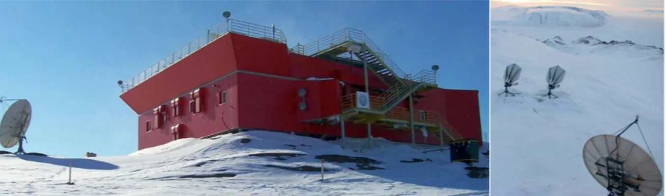
Figure 1: Accessibility map to Eureka (map credit: Northern Transportation Company Limited).
Figure 2: Eureka Weather Station (80◦N, 86◦W), emphasizing the star-photometer facility, near 0PAL Lab.
a modern residence capable of hosting about 50 people (Fig. 2). The cost of services provided by Eureka, as of April 2010,19 are: bed 250 $/day, three meals (professional cook, two choices) 230 $/day, electricity 1.143 $/kWh, workshop labor 150 $/h, small vehicle with driver 150 $/h, airport fees to land/takeoff a small aircraft 140 $. The land on which one wants to install any equipment is also an object of negotiation with EC and the station.
Electricity is currently provided by three 410 kWh Cummings diesel generators. Blackouts, during which, heating is cut off, can occur several times per year. In winter this is a life threatening event and, if longer than 12 h, the manager is compelled to order an evacuation, which in fact never happened. The fuel used by vehicles and generators is −40◦C rated, but it seems to work just fine down to −50◦C, which is about the lowest ground temperature. The station is serviced all year round by air, once a month, with food and other necessities. Taking advantage of being on the shore of the Slidre Fjord, the station is re-supplied almost every summer by an ice-breaker with construction materials, fuel, vehicles and other heavy items. Arrangements have to be made several months in advance in order to use this service. Depending on weight, the shipping of a sea container from Montreal to Eureka could cost a few thousands dollars. Eureka is also the last re-supplying point for North Pole expeditions, usually starting from the summertime-only research station on Ward Hunt Island,
Figure 3: PEARL Ridge Lab & C-band antenna (left, credit J. Drummond); 2 Ka- & C-band antennae (right).
at the northernmost tip of Canada (83◦060N, 74◦100W).20
Our organization, CANDAC, was formed in 2005 as a network of Canadian university and government researchers for investigating and monitoring the Arctic atmosphere. It currently operates PEARL (Polar Envi-ronment Atmospheric Research Laboratory), a complex of three facilities in the Eureka area: the Zero Altitude PEARL Auxilary Laboratory (0PAL) (Fig. 2), the PEARL Ridge Lab (Fig. 3, left) and the Surface and At-mospheric Flux, Irradiance and Radiation Extension (SAFIRE) laboratory. The PEARL ridge lab, formerly EC’s Arctic Stratospheric Ozone Observatory (Astro), is located 14 km from Eureka, at the summit of a 610 meter high ridge. The 0PAL site is located near the EC meteorological station while the SAFIRE station, which includes a 10 m measurement tower, is located near the airport. There are currently more than 25 CANDAC instruments in operation. Among them, the star-photometer facility is just near the 0PAL laboratory (Fig. 2), at 15 m elevation.
Until March 2012, CANDAC was operational all year long, with a permanent, on-site operator for maintaining all instruments. After this date, funding issues required that operations be limited to controlling instruments remotely (for those instruments that could be controlled remotely) accompanied by servicing missions (usually in October) and financed field campaigns (Polar sunrise campaign in the February to March period). Most recently, a moderate increase in operations funding has meant that a part time on-site operator could be employed and that measurement rates could be improved (the funding shortfall after March 2012 had a severe impact on measurement duty cycle).
In order to have adequate control of its instruments, CANDAC developed its own communication system, providing the most northern high speed internet connection. Actually, Eureka is about the northernmost location from where one can still see a geosynchronous satellite, which will be just few degrees over the horizon. Two connections are currently used: a C-band (4-8 GHz) link, at a cost of about 6 000 $/month for a ”high speed” traffic (∼380 kb/s) and several Ka-band (27-40 GHz) ”low speed” links for non real-time traffic, like data transfer. Until March 2014 the Ka-band links were provided for free by the Canadian Space Agency under the Government of Canada Capacity initiative. Having two connection options is useful for the reliability of the link (and the security of the equipment). There are problems during the summer months, especially in the high frequency band (Ka),21 when the air moisture and cloudiness increase. As the antennae are pointed close to the horizon,
the signals traverse a very long atmospheric path and are susceptible to absorption and scattering.
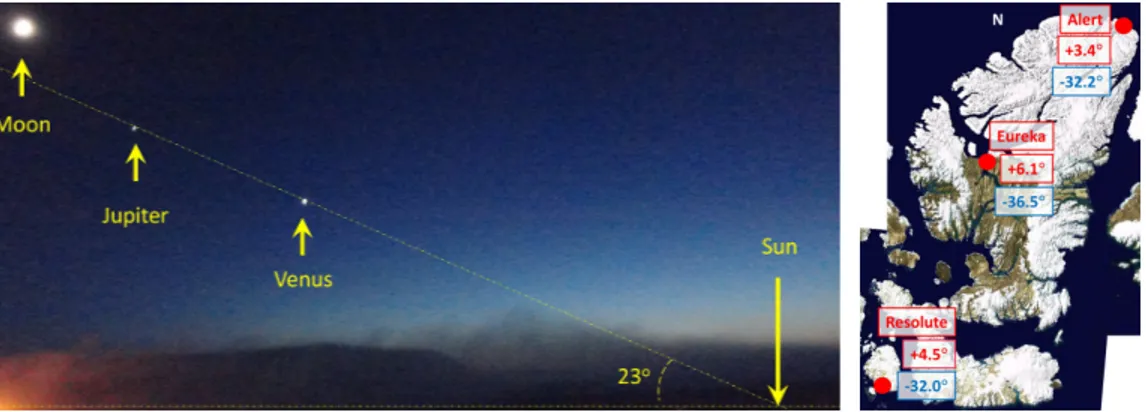
2.2 Observing conditions
Being near the North Pole, the night sky is characterized by particular conditions that affect measurement strategies inasmuch as the sun is never too far from the horizon. The position of the sun and the planets on or near the ecliptic plane means they share a common constrained geometry (Fig. 4, left) and motion in the sky. The moon is also never too high in the sky, as its orbiting plane is only 5◦off the ecliptic. Probably here, more than anywhere on Earth, it would have been easer for our ancestors to figure out the heliocentric system. The Polaris star is near the zenith, meaning that all the main solar system objects and most of the stars never rise or
Figure 4: Left: Sun, Moon and stars quasi-aligned on the ecliptic plane; fog on the fjord triggered by diesel generators exhaust. Right: July (red) & January (blue) daily mean surface temperature around Ellesmere Island.
set, rather they move almost parallel to the horizon. The site is also located near the magnetic North Pole, being practically in the center of the auroral oval. This means that auroras are very rarely seen on the horizon, so their contribution to the sky background brightness is not a significant issue in terms of star signal contamination.
The physical environment of Eureka results in anomalously colder winters and warmer summers in comparison with the rest of the Arctic. Fig. 4, right, shows the July (red) and January (blue) daily mean surface temperatures at Eureka and the two nearest stations. One could argue that the reason for this anomaly is a combination of the greater heat capacity of the sea (affecting more the coastal stations in summertime) and the caldera shape of the landscape around Eureka (a topographical condition that is suggested by the general features in the satellite image of Fig. 4). This would arguably allow for the accumulation of heat during the summer and prevent the mixing of the atmospheric boundary layer during the winter. Such a cold environment might help to lower the infrared sky brightness and open up new spectral windows for observing the stars.
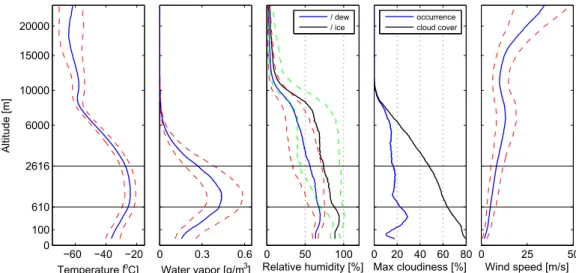
The wintertime (December, January, February) upper air radiosonde climatology (1994-2007) above Eureka is depicted in Fig. 5 & Fig. 6. The vertical scale is the square root of the altitude, which emphasizes parametric variations at both, low and high altitudes. The median (50% percentile) profiles, over the whole period, are represented with continuous lines (blue or black), while the 1st (25%) and 3rd (75%) percentiles are shown with dashed lines (red or green). Cloud occurrence (the blue curve of the Max cloudiness graph of Fig. 5) is computed only as an upper limit, inasmuch as the ice nucleation was considered here to start at 100% relative humidity over ice (RHi). In reality, due to aerosol acidification,22 cloud formation may be limited to values
higher than 150% RHi.23 The relative humidity over dew (RHd) is almost never 100% and pure water droplet
clouds are accordingly rare. Therefore, we express the cloud occurrence profile as the percentage of time one has ice nucleation at RHi >100%. The cloud cover profile (the solid black curve of the Max cloudiness graph
of Fig. 5) is computed then as the percentage of time one has any cloud occurrence above the current altitude. Cloud identification from the ground, based on an empirical OD threshold as low as 0.03, found 55% wintertime cloud cover at Eureka,24 so about 2/3 of our upper limit of 80% (Fig. 5). As an initial estimation, one may
then extrapolate such a 2/3 correction factor for the whole profile, which actually agrees very well with the observations.25
In order to better compare Eureka observing conditions with other astronomical sites, or the South Pole (as a reference for Antarctica, at 2 835 m elevation), we have also indicated two significant altitudes on the profiles of the Fig. 5 and Fig. 6: the PEARL Ridge Lab (610 m), near Eureka, and the highest peak on the Ellesmere Island (Barbeau, 2 616 m). This shows that the Ridge Lab is almost on top of the thermal inversion (Fig. 5, Temperature) and above the largest values of cloud occurrence (Fig. 5, Max cloudiness). On the other hand, Barbeau peak is above most of the moisture (Fig. 5, Water vapor). In addition, applying the 2/3 correction factor to the upper limit of 47% cloud cover, one may expect about 70% clear (photometric) sky in Barbeau, which is about what one finds at the best astronomical sites.26
The wind speed is generally very low, from almost negligible at sea level, to up to few m/s at the elevation
−60 −40 −20 0 100 610 2616 6000 10000 15000 20000 Temperature [oC] Altitude [m] 0 0.3 0.6
Water vapor [g/m3] Relative humidity [%]0 50 100 / dew / ice 0 20 40 60 80 Max cloudiness [%] occurrence cloud cover 0 25 50 Wind speed [m/s]
Figure 5: Radiosonde profiles above Eureka: winter median (DJF), 1994-2007; dashed lines: 1st& 3rdpercentiles.
0 2 4 6 8 10 12
10−1
100 101
Median year 1994−2007 (dots: 1st & 3rd perc.)
PWV (mm) Months SP 2835 m EU 2616 m EU 610 m EU 20 m
Figure 6: Radiosonde measurements above Eureka: wintertime (DJF) wind direction occurrences over a period extending from 1994 to 2007 (left); vertical integration of Precipitable Water Vapor (PWV): median for the same period (right). EU & SP stand for Eureka & South Pole, respectively.
of the Ridge Lab and Barbeau peak (Fig. 5, Wind speed). The air circulation above Eureka is presented in the left-hand chart (65 × 65 pixels) of Fig. 6. The color scale shows the percentage of radiosonde samples when the wind, of any speed, arrives from the directions and altitudes covered by a pixel (∼ 6◦/pixel). In order to emphasize the main air circulation pattern, one also limits our analysis to the high speed winds (>10 m/s). Their 50% occurrence (from all the radiosonde samples) are enclosed within the black contours.
One can then identify stable, high speed, northwesterly winds in the stratosphere, most probably part of the polar vortex, at altitudes higher than about 10 000 m. From polar (Hadley) cell air circulation considerations, one should expect upper tropospheric southerlies and lower tropospheric northesterlies. While one can identify northesterlies in the whole troposphere, down to the Ridge Lab elevation (wind direction at ∼ 45◦ in the chart of Fig. 6), the high altitude southerlies are less obvious. On the other hand, one can observe evident high speed southerlies (enclosed in the black contours) below the Ridge Lab elevation. It may mean that Eureka is too close to the pole for experiencing the expected air circulation pattern, or so close to the pole that one might have an additional inverted polar cell. On the other hand, upper tropospheric northesterlies (instead of southerlies) may also be due to local semi-permanent synoptic features, like the cyclones traveling north along the Baffin Bay, between Canada and Greenland, and east of Eureka.27 Bellow the Ridge Lab elevation, those northeasterlies
are quenching down, having a less stable direction, most probably due to the landscape, inasmuch as Eureka is downhill and south of the Ridge Lab. In addition, the low elevation southerlies tend to turn left, to become
Figure 7: Events of typical cloudy filaments in Eureka coming from the south: every picture is a different event, both raws show similar time of day, while left to right show various times from morning to after-noon (views from south-east to south-west).
easterlies, when approaching sea level. According to the Ekman theory, this means that they are associated with occasional low pressure systems west of Eureka and above the Canadian archipelago, where one usually finds the highest presence of high pressure systems during the winter.27 From our experience, wintertime cloudy events are generally also from the south (Fig. 7), probably due to such systems. The generally calm atmosphere of the winter is abruptly changed in spring, usually during the month of March, by northwesterly blizzards of more than 10 m/s wind speed at the surface.
The vertically integrated water content, expressed as Precipitable Water Vapor (PWV) in the right-handed graph of Fig. 6, emphasizes a very dry winter atmosphere. This is computed from the twice daily radiosonde measurements, as a 30 day running median, so occasional high frequency events of short duration and high moisture content are likely filtered out. At an altitude comparable with other astronomical sites, one finds values of PWV ∼0.4 mm for Barbeau peak. This is comparable with the South Pole (0.1-0.2 mm) and drier than the current estimation for Summit, Greenland (0.9 mm).28 Even the Ridge Lab, at 1.5 − 2 mm, is comparable with
the best astronomical sites in their dry season29.30
Semi-transparent ice clouds, mainly found at mid-latitudes as high altitude cirrus, are often neglected in cloud cover calculations. They are actually present more than 40% of the time.31 During the polar night they have a pan-polar presence 50-60% of the time and occur at any altitude, including ground level.22 Such optically thin ice clouds (TIC), OD < 3, are a major motivation for star-photometry observations at Eureka. From our experience, TICs usually originate in the south, probably driven by low pressure systems west of Eureka (Fig. 7 shows their South-North filamentary pattern). As shown in Fig. 5, one also has an increased cloud occurrence near sea level. Low laying TICs, or occasional supercooled liquid fog, are mostly found along the fjords (Fig. 8, a), but the northeasterly winds may sometimes advect them uphill to the Ridge Lab.
While being vital for the station, the diesel generators also vent exhaust fumes into the air. The exhaust triggers cloud nucleation and can produce fog just above the station (Fig. 8, b), particularly at very low temper-atures (< −40◦C), a phenomenon that occurs often during the polar winter at Eureka. The lowest temperatures
occur during clear sky scenes, with northeasterly winds moving the fog southwest, towards the fjord. A lesser exhaust, produced by the generators at the airport, also moves above the station and star-photometer, towards the fjord, at a higher elevation (∼ 100 m). Beyond adding an unwanted contribution to the optical depth, such fog also backscatters the streetlight, contributing therefore to the sky background pollution. Fig. 8 (b) shows the Eureka complex light pollution, below −40◦C. Some of the clear sky scenes, appropriate for aerosol observations, are accordingly affected by the local pollution.
Snow cover is basically everywhere on the ground, generally being dry (no mixed phase), made up of small crystals, with the consistency of a powder (Fig. 8, c). This means that even the mildest air currents can induce blowing crystals. For this reason, the ground snow preserves a fresh consistency, which could be an explanation of the high albedo. Actually the albedo is so high, that even starlight is sufficiently bright to visually perceive the