Pépite | Méthode d'élément composite pour la modélisation de l'écoulement transitoire des eaux souterraines dans les milieux fracturés et son application au problème de stabilité de la pente

Texte intégral

(1)Thèse de Xiaoping Hou, Lille 1, 2017. N° d’ordre:. Année 2017. UniversitéLille 1 Sciences et Technologies Laboratoire Génie Civil et géo-Environnement Ecole doctorale Sciences Pour l’Ingénieur. THÈSE Pour l’obtention du grade de Docteur de L’Université des Sciences et Technologies de Lille Discipline: Génie Civil Sous le titre de:. Composite Element Method for Modelling Transient Groundwater Flow in Fractured Media and its Application to Slope Stability Problem par. Xiaoping HOU Présentée et soutenue publiquement le 29 Juin 2017 Devant le jury constituéde: SHAHROUR Isam. Professeur, UniversitéLille 1. Directeur de thèse. CHEN Shenghong. Professeur, Wuhan University. Directeur de thèse. AL HEIB Marwan. Professeur, Ecole des Mines Nancy. Rapporteur. WU Aiqing. Professeur, Yangtze River Scientific Rapporteur Research Institute. ABBAS Oras. Docteur, A+Métrologie -groupe Apave Examinateur. FU Shaojun. Professeur, Wuhan University. © 2017 Tous droits réservés.. Examinateur. lilliad.univ-lille.fr.

(2) Thèse de Xiaoping Hou, Lille 1, 2017. © 2017 Tous droits réservés.. lilliad.univ-lille.fr.

(3) Thèse de Xiaoping Hou, Lille 1, 2017. Résumé Ce travail de thèse propose un modèle numérique complet pour l'écoulement transitoire des eaux souterraines dans les milieux poreux et fracturés et son application sur l’analyse de la stabilité des pentes sous l’effet d’une diminution du niveau de l’eau dans un réservoir. L’écouement de l’eau dans les milieux fracturés est complexe, en raison de la présence d'un grand nombre de fractures et de fortes variations dans les propriétés géométriques et hydrauliques de ces milieux. La thèse est organisée en six chapitres. Le premier chapitre pésente les problèmes abordés et les objectifs de la thèse. Le 2nd chapitre présente une synthèse des analyses numériques de l'écoulement dans les milieux fracturés et de ses effets sur la stabilitédes pentes. Le 3ème chapitre présente le développment d’un modèle numérique d'écoulement transitoire saturédans des milieux fracturés avec une surface libre en utilisant la méthode des éléments composites (CEM). Le 4ème chapitre présente un modèle numérique d'écoulement transitoire àsaturation variable, dans les milieux fracturés àl'aide du CEM. Le 5ème chapitre présente une étude de la stabilitédes pentes sous l’effet de variation des paramètres hydrauliques et de résistance des sols, et da géométrie des pentes. Le 6ème chapitre présente une étude paramétrique de l'influence des caractéristiques de fracture sur l'écoulement transitoire et la stabilité d’une pente soumise àdes conditions de diminution. Mots-clés: écoulement des eaux souterraines; milieux fracturés; écoulement àsaturation variable; surface libre; méthode élément composite; stabilité de la pente; méthode d'équilibre limite; vidange rapide. I © 2017 Tous droits réservés.. lilliad.univ-lille.fr.

(4) Thèse de Xiaoping Hou, Lille 1, 2017. Abstract This thesis presents a comprehensive numerical method for analyzing transient groundwater flow in porous and fractured media and its application to the analysis of the stability of soil and rock slopes subjected to transient groundwater flow induced by reservoir drawdown conditions. Compared to that of porous media, the analysis of flow in fractured media is relatively complex, due to the presence of a large number of fractures and strong variations in geometric and hydraulic properties. The thesis is organized in six chapters. Chapter 1 presents the issues to be addressed and the thesis objectives. Chapter 2 discusses basic theories related to the numerical analysis of groundwater flow in fractured media and its effects on slope stability. Chapter 3 develops the numerical model of transient, saturated flow in fractured media with a free surface using the composite element method (CEM). Chapter 4 presents the numerical model of transient, variably-saturated flow in fractured media using the CEM. Chapter 5 includes an investigation of the stability of homogeneous soil slopes under drawdown conditions, depending on the drawdown rate, hydraulic and strength parameters of soils, and slope geometry. The last chapter presents a parametric study on the influence of fracture characteristics on transient flow and stability of layered rock slope subjected to drawdown conditions. Keywords: groundwater flow; fractured media; variably-saturated flow; free surface; composite element method; slope stability; limit equilibrium method; rapid drawdown. II © 2017 Tous droits réservés.. lilliad.univ-lille.fr.

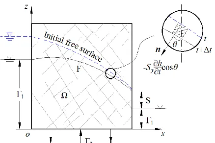
(5) Thèse de Xiaoping Hou, Lille 1, 2017. Summary The study of groundwater flow in fractured media can be distinct from that of flow in porous media due to the complex geologic configurations of fractured media. In modelling study of flow in fractured media, the discrete fracture approach is a preferable approach because it has the potentiality to describe the fractures in more detail. However, the difficulty of using this approach is the explicit representation of the geometry of fractured media, which, in numerical modelling, refers to the discretization of the fractured media into computational meshes. The composite element method (CEM) has a prominent advantage on the discretization, so it is quite suited for developing the numerical model of groundwater flow in fractured media, which is the first task of this work. The analysis of groundwater flow often plays an important role in the solution of slope stability problems. The drawdown condition is a common scenario in slope stability. However, the current investigations for the drawdown condition are not deep enough. One of the main reasons is that the pore-water pressures within the slopes during drawdown are not accurately estimated. The second task of this work is to use the developed numerical model to obtain accurate pore-water pressures and then to make reasonable evaluation for the stability of slopes subjected to drawdown conditions. The above contents are presented in Chapter 1. In Chapter 2, some basic problems involved in the numerical analyses of groundwater flow in fractured media and its effects on slope stability are considered. In the aspect of the groundwater flow in fractured media, the basic law of single fracture flow, the modelling approaches for flow in fractured media, the composite element method for analyzing discretely-fractured media, and the flow characteristics of variably-saturated system, are respectively discussed. The problems existing in the previous modelling studies of flow in fractured media are pointed out, as well as the capability of the CEM in solving these problems. Then, the research progress of the CEM in analyzing the fractured media is given a certain introduction. In the aspect of the effects of groundwater flow on slope stability, three actions of groundwater on slope stability are described, and the limit equilibrium and the numerical methods for stability analysis are summarized. Particular mention is made of the importance of the reservoir’s rapid drawdown to slope stability analysis. The discussion of these problems provides theoretical bases for subsequent studies. In Chapter 3, a three-dimensional numerical model for simulating transient, saturated. III © 2017 Tous droits réservés.. lilliad.univ-lille.fr.

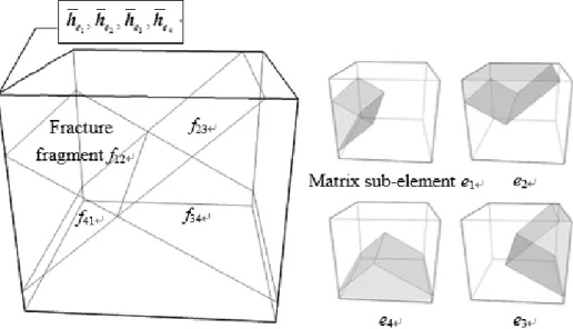
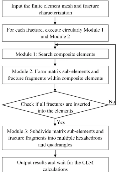
(6) Thèse de Xiaoping Hou, Lille 1, 2017. flow in fractured media with a free surface is constructed using the CEM. The model does not require generation of specific elements for representing fractures, but, instead, inserts the fractures into the elements so as to form the composite elements. The governing equation for the composite element containing both fractures and matrix is derived by using the variational principle. It provides accurate descriptions of fracture flow, matrix flow and exchange of water between fractures and matrix. The relevant solution algorithms are presented, including those of CEM pre-processing, numerical integral calculation, treatment of boundary conditions and solving large, sparse, symmetric system of equations. In particular, an iterative scheme for locating the shifting free surface is introduced. The validity and reliability of the model are verified by a synthetic example. The capability of the model is demonstrated by simulations of the flow problems in complicated fractured aquifers. In Chapter 4, the CEM is used to further develop the numerical model for simulating transient, variably-saturated flow in fractured media. Since the constitutive relations (saturation‒pressure head and relative permeability‒saturation relations) for fractures may be highly linear and different than those for matrix, a fast and stable iterative scheme using under-relaxation technique is implemented to solve the variably-saturated flow equations. The techniques of mass matrix lumping and adaptive time stepping are used to further enhance accuracy and efficiency. The effectiveness of the developed model is verified by simulations of one-dimensional infiltration into dry soils and the synthetic example which was discussed in Chapter 3 and simulated by assuming water flowing only in the saturated zone with a shifting free surface. The simulation results are compared with the semianalytical solution and those obtained from a commercial software COMSOL. Several illustrative problems that demonstrate the complexity of variably-saturated flow in fractured aquifers are presented in the end of this chapter. In Chapter 5, the stability of homogeneous soil slopes under reservoir drawdown conditions is studied. The composite element modelling of transient, saturated flow with a free surface (assuming non-deforming slope media) is used to calculate the transient free surfaces and pore-water pressure distributions in the slopes during reservoir drawdown. Using the calculated pore-water pressure distributions, the limit equilibrium analyses are then conducted to derive the variations of the safety factor of homogeneous soil slopes during drawdown. It has been found from the theoretical analyses of transient flow and slope stability that the variation of safety factor of the slopes during drawdown depends on the. IV © 2017 Tous droits réservés.. lilliad.univ-lille.fr.

(7) Thèse de Xiaoping Hou, Lille 1, 2017. hydraulic index k/(Syv) and the strength index c’/(γHtanφ’). Therefore, these two indexes are employed in systematically investigating the influence of various drawdown rates and material parameters on transient flow and stability of homogeneous soil slopes. These investigation results serve for the formulation of criteria for judging rapid drawdown conditions. In this criteria, the rapid drawdown is defined as the one which results in more than 4% reduction in the safety factor of homogeneous soil slopes during reservoir drawdown. Hopefully, this criteria can be adopted in engineering practice. In Chapter 6, the stability of layered rock slopes under reservoir drawdown conditions is studied. These slopes are assumed to contain one group of evenly spaced, parallel and persistent fractures (inter-layers). Due to the presence of the fractures, the transient flow processes in the slopes under drawdown conditions are different from those in the homogenous soil slopes studied in Chapter 5. This chapter conducts a parametric study using the CEM, to specially investigate the influence of various geometric characteristics of the fracture group on transient flow in the layered rock slopes during drawdown. These characteristics include fracture aperture, spacing, and dip angle. Then, the pore-water pressures obtained by transient flow simulations are used as groundwater conditions for slope stability analyses to obtain the variation of the safety factor of the layered rock slopes during drawdown. The investigation results provide quantitative verification of the impact of the reservoir drawdown on the stability of rock slopes with certain geological structure features. Since there are a large number of factors that may control groundwater flow in rock slopes, it is only possible in this work to study one of the simplest rock slope types (i.e., layered rock slope with persistent fractures), and to give a small amount of quantitative verification. However, the methodologies, including the CEM and the combined CEM-LEM analysis approach, are available for further investigations of the stability of complex rock slopes that suffer from the reservoir drawdown conditions.. V © 2017 Tous droits réservés.. lilliad.univ-lille.fr.

(8) Thèse de Xiaoping Hou, Lille 1, 2017. Table of Contents Résumé.............................................................................................................................................. I Abstract ............................................................................................................................................ II Summary ......................................................................................................................................... III Table of Contents ............................................................................................................................VI List of Tables .................................................................................................................................... X List of Figures .................................................................................................................................XI Chapter 1 Introduction ...................................................................................................................... 1 1.1 Introduction and motivation ................................................................................................ 1 1.2 Objectives and scope ........................................................................................................... 4 1.3 Outline of thesis .................................................................................................................. 5 References ................................................................................................................................. 7 Chapter 2 Basic Considerations ...................................................................................................... 10 2.1 Introduction ....................................................................................................................... 10 2.2 Flow through single fractures............................................................................................ 10 2.2.1 Classical cubic law ................................................................................................. 10 2.2.2 Correction of the cubic law .................................................................................... 11 2.3 Flow in fractured media .................................................................................................... 13 2.3.1 From single fractures to fractured media ............................................................... 13 2.3.2 Modelling approaches for flow in fractured media ................................................ 13 2.3.3 The use and weakness of discrete fracture network model .................................... 14 2.4 Composite element method ............................................................................................... 16 2.4.1 Basic principle of the CEM .................................................................................... 16 2.4.2 Research progress of the CEM ............................................................................... 18 2.5 Flow in variably-saturated systems ................................................................................... 18 2.6 Effects of groundwater on slope stability .......................................................................... 20 2.6.1 Mechanical action of groundwater ......................................................................... 20 2.6.2 Softening and erosion actions of groundwater ....................................................... 20 2.6.3 Rapid reservoir drawdown ..................................................................................... 20 2.7 Stability analysis methods ................................................................................................. 21. VI © 2017 Tous droits réservés.. lilliad.univ-lille.fr.

(9) Thèse de Xiaoping Hou, Lille 1, 2017. 2.7.1 Limit equilibrium methods ..................................................................................... 21 2.7.2 Numerical methods ................................................................................................ 22 2.8 Conclusions ....................................................................................................................... 23 References ............................................................................................................................... 25 Chapter 3 Composite Element Method for Modelling Transient, Saturated Flow in Fractured Media with a Free Surface ................................................................................................................................. 30 3.1 Introduction ....................................................................................................................... 30 3.2 Mathematical descriptions of transient, saturated flow problem....................................... 32 3.3 Composite element model construction ............................................................................ 34 3.3.1 Hydraulic head within composite element ............................................................. 34 3.3.2 Composite element formulation ............................................................................. 35 3.4 Relevant solution algorithms ............................................................................................. 38 3.4.1 CEM pre-processing............................................................................................... 38 3.4.2 Numerical integral calculation ............................................................................... 39 3.4.3 Treatment of boundary conditions.......................................................................... 41 3.4.4 Solving large sparse symmetric equations ............................................................. 42 3.5 Verification example ......................................................................................................... 42 3.5.1 Flow in a synthetic fractured rock mass ................................................................. 42 3.6 Simulations of flow problems in complicated, saturated fractured aquifers ..................... 48 3.6.1 Flow in a 2D fractured network ............................................................................. 48 3.6.2 Transient groundwater flow in a rock slope following reservoir rapid impounding ................................................................................................................................................. 50 3.7 Conclusions ....................................................................................................................... 52 References ............................................................................................................................... 56 Chapter 4 Composite Element Method for Modelling Transient, Variably-Saturated Flow in Fractured Media ...................................................................................................................................... 58 4.1 Introduction ....................................................................................................................... 58 4.2 Mathematical descriptions of transient, variably-saturated flow problem ........................ 59 4.3 Composite element model development ........................................................................... 60 4.3.1 Constitutive relations for matrix and fractures ....................................................... 60 4.3.2 Fracture-matrix interaction area factor ................................................................... 62. VII © 2017 Tous droits réservés.. lilliad.univ-lille.fr.

(10) Thèse de Xiaoping Hou, Lille 1, 2017. 4.3.3 Composite element formulation ............................................................................. 62 4.4 Key techniques for improving numerical accuracy and efficiency ................................... 64 4.4.1 Under-relaxation iteration ...................................................................................... 64 4.4.2 Mass matrix lumping.............................................................................................. 65 4.4.3 Adaptive time stepping ........................................................................................... 65 4.5 Verification examples ........................................................................................................ 66 4.5.1 1D infiltration into dry soil..................................................................................... 66 4.5.2 Flow in a synthetic fractured rock mass ................................................................. 67 4.5.3 Vertical drainage of a fractured tuff column ........................................................... 67 4.6 Simulation of flow problem in complicated, variably-saturated fractured aquifer ........... 72 4.6.1 Transient flow in an aquitard-aquifer system under recharge and pumping .......... 72 4.7 Conclusions ....................................................................................................................... 77 References ............................................................................................................................... 80 Chapter 5 Investigation of Stability of Homogeneous Soil Slopes Under Drawdown Conditions . 83 5.1 Introduction ....................................................................................................................... 83 5.2 Theories and approaches used for this investigation ......................................................... 85 5.2.1 Analysis of transient flow in a 2D slope................................................................. 85 5.2.2 Analysis of slope stability with respect to circular sliding ..................................... 86 5.2.3 Design specifications for allowable SF and acceptable reduction in SF ................ 88 5.3 Investigation of drawdown in homogeneous soil slopes ................................................... 89 5.3.1 The decline of the free surface within slopes during drawdown ............................ 90 5.3.2 The variation in SF of slopes during drawdown .................................................... 92 5.3.3 Comparisons between old and new criteria for judging rapid drawdown .............. 93 5.4 Charts for quick judgment of rapid drawdown in homogeneous soil slopes..................... 95 5.5 Conclusions ....................................................................................................................... 99 References ............................................................................................................................. 101 Chapter 6 Investigation of Stability of Layered Rock Slopes Under Drawdown Conditions ....... 102 6.1 Introduction ..................................................................................................................... 102 6.2 Analysis of slope stability with respect to planar sliding ................................................ 103 6.3 Investigation of drawdown in layered rock slopes .......................................................... 104 6.3.1 Parameters influencing transient flow in layered rock slopes .............................. 105. VIII © 2017 Tous droits réservés.. lilliad.univ-lille.fr.

(11) Thèse de Xiaoping Hou, Lille 1, 2017. 6.3.2 Parameter setting and analysis protocols.............................................................. 106 6.3.3 Sensitivity analyses of fracture characteristics ..................................................... 107 6.4 Conclusions ..................................................................................................................... 112 References ............................................................................................................................. 114 Chapter 7 Conclusions and Recommendations ............................................................................. 115 7.1 Conclusions ..................................................................................................................... 115 7.2 Recommendations for future research............................................................................. 116. IX © 2017 Tous droits réservés.. lilliad.univ-lille.fr.

(12) Thèse de Xiaoping Hou, Lille 1, 2017. List of Tables Table 2.1 Some expressions of C and bc ......................................................................................... 12 Table 2.2 Advantages and disadvantages of each modelling approach for flow in fractured media (refer to [National Research Council,1996] and [Cook, 2003]) .............................................. 15 Table 2.3 Equilibrium conditions required for each limit equilibrium method [Chen, 2015] ......... 22 Table 2.4 Inter-slice force characteristics and relationships for each limit equilibrium method [Chen, 2015] ....................................................................................................................................... 22 Table 3.1 Parameters of four groups of fractures and their probability models .............................. 51 Table 4.1 Parameters of three groups of fractures and their probability models ............................. 74 Table 4.2 Tabular data describing the saturation‒pressure head and relative permeability‒saturation relations ................................................................................................................................... 75 Table 5.1 Allowable safety factors for slopes at reservoir area [National Development and Reform Commission of P.R. China, 2006] ........................................................................................... 89 Table 5.2 Input parameters for drawdown analyses of homogeneous soil slopes shown in Figures 5.3 and 5.5 ............................................................................................................................... 90 Table 5.3 Values of k/(Syv) and c’/(γHtanφ’) for quick judgment of rapid and slow drawdown in homogeneous soil slopes with different geometrical features ................................................. 97 Table 6.1 Classification of layered rock mass and associated failure mode (referring to [Chen, 2015], and slightly modified) ........................................................................................................... 103 Table 6.2 Input parameters for parametric analyses of fracture characteristics shown in Figure 6.36.7.......................................................................................................................................... 107. X © 2017 Tous droits réservés.. lilliad.univ-lille.fr.

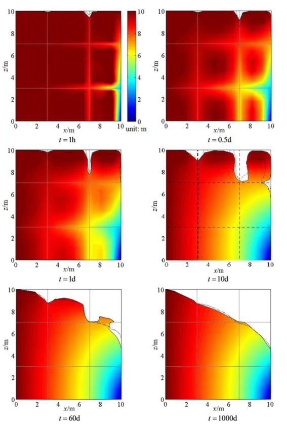
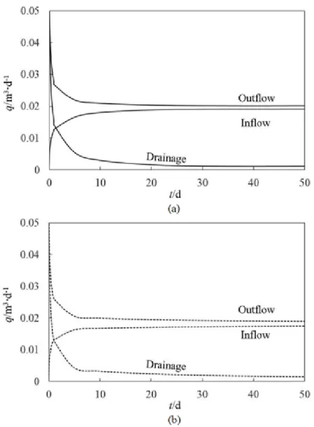
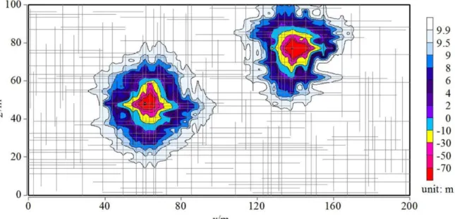
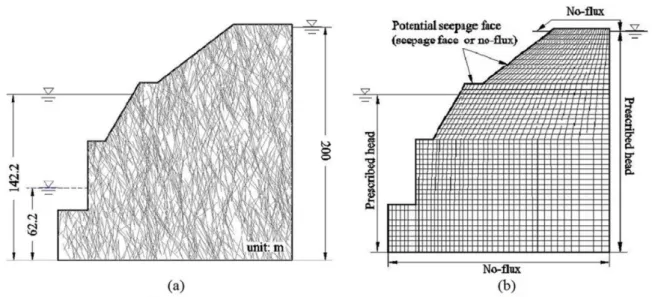
(13) Thèse de Xiaoping Hou, Lille 1, 2017. List of Figures Figure 2.1 Conceptual models of a single fracture: (a) a pair of smooth, parallel plates; and (b) a pair of rough-walled surfaces [Brush, 2001] .......................................................................... 11 Figure 2.2 Two types of composite elements and their internal sub-elements ................................ 17 Figure 3.1 Cross section of an unconfined fractured aquifer with four types of boundaries: the prescribed head boundary Γ1, the prescribed flux boundary Γ2, free surface F and seepage face S .............................................................................................................................................. 33 Figure 3.2 A composite element containing four matrix sub-elements and four fracture fragments ................................................................................................................................................. 34 Figure 3.3 Workflow of the pre-processor to insert the fracture surfaces into the generated mesh 39 Figure 3.4 Synthetic fractured rock mass ........................................................................................ 43 Figure 3.5 Two computational meshes respectively used in (a) composite element model, and (b) COMSOL ................................................................................................................................ 43 Figure 3.6 Evolution of the hydraulic head on the profile y=5 m using composite element model in case 1 ....................................................................................................................................... 45 Figure 3.7 Comparisons of the hydraulic head distributions along the centerline at different times obtained with (a) composite element model, and (b) COMSOL in case 1 .............................. 46 Figure 3.8 Evolution of the hydraulic head on the profile y=5 m using composite element model in case 2 ....................................................................................................................................... 47 Figure 3.9 Comparisons of inflow, outflow and drainage fluxes in the domain obtained with (a) composite element model, and (b) COMSOL in case 2 .......................................................... 48 Figure 3.10 Hydraulic head distribution in the domain after three-year pumping obtained with the composite element model ........................................................................................................ 50 Figure 3.11 Fractured rock slope: (a) geometry, and (b) computational mesh ................................ 51 Figure 3.12 Evolution of the hydraulic head in the fractured rock slope using the composite element model....................................................................................................................................... 53 Figure 3.13 Groundwater velocity vectors in the fractured rock slope obtained with the composite element model ......................................................................................................................... 54 Figure 4.1 Distributions of the pressure head along depth at t=6 h................................................. 68 Figure 4.2 Number of iterations in each time step required to achieve convergence...................... 68. XI © 2017 Tous droits réservés.. lilliad.univ-lille.fr.

(14) Thèse de Xiaoping Hou, Lille 1, 2017. Figure 4.3 Evolution of the hydraulic head on the profile y=5 m using composite element model in case 2 (recalculated by simulating transient, variably-saturated flow) ................................... 69 Figure 4.4 Comparisons of inflow, outflow and drainage fluxes in the domain obtained with the two composite element models respectively developed in Chapter 3 and in Chapter 4 and COMSOL ................................................................................................................................................. 70 Figure 4.5 A fractured tuff column .................................................................................................. 70 Figure 4.6 Relations between (a) saturation, (b) relative permeability, and (c) effective area factor and pressure head .................................................................................................................... 71 Figure 4.7 Variations of the pressure head with time at four given points in (a) case 1, and (b) case 2............................................................................................................................................... 73 Figure 4.8 A aquitard-aquifer system .............................................................................................. 74 Figure 4.9 Contours of the hydraulic head at y=45 m (a) initially, and (b) after 500 d pumping .... 77 Figure 4.10 Location of the free surface after 500 d pumping ........................................................ 78 Figure 5.1 Forces acting on a slice through the sliding mass enclosed by a circular slip surface ... 87 Figure 5.2 A drawdown problem in a homogenous soil slope ........................................................ 89 Figure 5.3 The calculated free surfaces at different drawdown levels HD/H under conditions of k/(Syv)=0.1, 1, 10, 100 and 1000 ............................................................................................. 91 Figure 5.4 Relation between k/(Syv) and (HD-ΔHD)/HD at end of drawdown.................................. 91 Figure 5.5 Variations of the computed SF/tanφ’ with HD/H, under conditions of k/(Syv)=0.1, 1, 10, 100 and 1000, when c’/(γHtanφ’)=0.137 ................................................................................ 93 Figure 5.6 Relation between k/(Syv) and relative reduction in minimum SF caused by drawdown 94 Figure 5.7 Conditions for rapid and slow drawdown in homogeneous soil slopes with L/H=1.2 and m=2 ......................................................................................................................................... 94 Figure 5.8 Charts for quick judgment of rapid and slow drawdown in homogeneous soil slopes with different geometrical features.................................................................................................. 97 Figure 6.1 Forces acting on a sliding mass enclosed by a planar slip surface .............................. 104 Figure 6.2 A drawdown problem in a layered rock slope containing one group of fractures dipping away the slope ....................................................................................................................... 105 Figure 6.3 Free surfaces and contours of the hydraulic head at end of drawdown in the layered rock slopes with different fracture apertures: (a) b=12.1 μm; (b) b=26.1 μm; (c) b=56.1 μm; and (d) b=121.0 μm ........................................................................................................................... 108. XII © 2017 Tous droits réservés.. lilliad.univ-lille.fr.

(15) Thèse de Xiaoping Hou, Lille 1, 2017. Figure 6.4 Variations of the computed SF/tanφ’ with HD/H for the layered rock slopes with different fracture apertures: (a) b=12.1 μm; (b) b=26.1 μm; (c) b=56.1 μm; and (d) b=121.0 μm ...... 109 Figure 6.5 Free surfaces and contours of the hydraulic head at end of drawdown in the layered rock slopes with different fracture spacings: (a) d=1.0 m; (b) d=2.5 m; (c) d=5.0 m; and (d) d=10.0 m ........................................................................................................................................... 110 Figure 6.6 Variations of the computed SF/tanφ’ with HD/H for the layered rock slopes with different fracture spacings: (a) d=1.0 m; (b) d=2.5 m; (c) d=5.0 m; and (d) d=10.0 m ....................... 111 Figure 6.7 Free surfaces and contours of the hydraulic head at end of drawdown in the layered rock slopes with different fracture dip angles: (a) ψ=30°; (b) ψ=40°; (c) ψ=50°; and (d) ψ=60°. 111. XIII © 2017 Tous droits réservés.. lilliad.univ-lille.fr.

(16) Thèse de Xiaoping Hou, Lille 1, 2017. Chapter 1 Introduction 1.1 Introduction and motivation Groundwater flow is a ubiquitous phenomenon in the Earth’s crust, and the analysis of this phenomenon plays an important role in solution of many geotechnical problems, especially those concerning the stability analyses of slopes. Compared to that in porous media, flow of groundwater in rocky media (which are usually fractured) is relatively complex. The complexity is mainly resulted from the presence of a large number of fractures and the strong variations in geometric and hydraulic properties, such as fracture aperture, shape, orientation, position, and hydraulic conductivity. Thus, different—though in many cases complementary—theories and methods must be considered. This thesis is aimed at developing a comprehensive numerical method for analyzing groundwater flow in porous media and fractured media. Then, the method is applied to the problem of the stability analyses of soil and rock slopes subjected to groundwater flow, which is the second aim of this thesis. The modelling is a significant component for understanding the hydraulic behavior of the media. The finite element method (FEM) [Zienkiewicz et al., 1966] is the most commonly used method for flow analysis. According to different ways of fracture simulation, the existing numerical models for solution of flow in fractured media can be grouped into two categories: one is the implicit (continuum) model which takes the impact of fractures into the hydraulic properties of equivalent porous media but ignores their exact positions (e.g. [Barenblatt et al., 1960; Warren and Root, 1963; Snow, 1969; Duiguid and Lee, 1977; Long et al., 1982; Peters and Klavetter, 1988; Narasimhan and Pruess, 1988; Carrera et al., 1990]); the other is the explicit (discrete fracture) model which uses special elements to exactly simulate the geometric and hydraulic properties of fractures (e.g. [Louis, 1972; Schwartz et al., 1983; Andersson et al., 1984; Andersson and Dverstorp, 1987; Cacas et al., 1990; Hyman et al., 2015]). The former can be applied into large-scale engineering problems with a large number of fractures, whereas the latter has the potentiality to describe the fractures in more detail and hence gives more accurate solution. From the practitioner’s point of view, the main difficulty in the explicit simulation of fractures is to generate finite element meshes representing the heterogeneous media, which are used to solve various engineering problems based on the FEM. This arises from two aspects: 1 © 2017 Tous droits réservés.. lilliad.univ-lille.fr.

(17) Thèse de Xiaoping Hou, Lille 1, 2017. . On the one hand, there are a large number of fractures with different sizes and that are interlaced mutually.. . On the other hand, the specific elements representing fractures have definite nodes in their location, and some of these nodes should be the common ones of the surrounding rock elements.. The difficulty, along with complex configuration of geotechnical structures such as dam foundation, rock slope and underground cavern, leads to time-consuming and tedious preprocessing work. The composite element method (CEM) [Chen et al., 2002] has been proposed to solve the difficulty discussed above, and has been implemented for rock fractures, rock bolts, drainage holes and cooling pipes [Chen and Qiang, 2004; Chen et al., 2004a, 2004b, 2011; Chen and Feng, 2006; Hou et al., 2015]. A prominent feature of the CEM is to place the fractures, or bolts, or drainage holes, or cooling pipes inside the elements. In this way less restraint is imposed on the mesh generation for complicated geotechnical structures with considerable amount of fractures, bolts, drainage holes and cooling pipes. The first task of this work is to use the CEM to develop numerical model of groundwater flow in complex fractured media. This model can be placed into a category of the explicit model, because the fractures are explicitly simulated within the composite elements. If there are no fractures, the CEM can be automatically degenerated into the FEM, which is another prominent feature of the CEM, and then, the model can be used to solve flow problems in porous media. It has been widely recognized that groundwater flow—or specifically speaking, its resulting actions—have a significant effect on the stability of slopes [Hodge and Freeze, 1977]. The pore-water pressure undermines the stability by diminishing the shear strength on the potential slip surface. The pore-water pressure in tension cracks or nearly vertical fissures also reduces the stability by additional slip driving forces. In general, the vast majority of natural slopes have stabilized after long-term geological effects (including longterm steady flow of groundwater). However, when slopes are subjected to surrounding environmental changes, such as rainfall infiltration or reservoir level fluctuation, the porewater pressures in the slopes will change, thus changing the original balance situation. For a slope originally approaching or being in a limit stability state, this change may cause the instability of the slope. Estimation of pore-water pressures plays an important role in the slope stability analysis. Landslide induced by rapid drawdown of reservoir is one of the common geological hazards. When the reservoir level is high, the hydrostatic pressures help to stabilize the slope 2 © 2017 Tous droits réservés.. lilliad.univ-lille.fr.

(18) Thèse de Xiaoping Hou, Lille 1, 2017. adjacent to the reservoir. A reduction of the reservoir level has two effects: a decrease in the external stabilizing hydrostatic pressures and a modification of the internal pore-water pressures. If the reservoir level is lowered rapidly, the pore water within the slope cannot drain in time so that the pore-water pressures in the slope still remain high values. This may lead to the temporarily increased hydraulic gradients and cause that the stability of the slope cannot be sustained. Eventually a failure occurs. Stability analysis of the slope subjected to reservoir’s rapid drawdown condition has become one of the most important considerations in the design of embankment dam and the stabilization of reservoir bank slope [National Development and Reform Commission of P.R. China, 2006; U.S. Army Corps of Engineers, 2003]. However, the current stability computations for rapid drawdown condition are mostly based on certain assumptions, thus resulting in insufficient understanding of the impact of reservoir drawdown on the slope stability. The main assumptions and the resulting insufficiency are as follows: . Firstly, the concept of “sudden drawdown” (or “fully rapid drawdown”) is widely used for slopes with various hydrogeological, and soil and rock conditions [Wright and Duncan, 1987]. The so-called “sudden drawdown” refers to the change in reservoir level happening without allowing the time needed for drainage of slope soils or rocks, and thus the groundwater level or the free surface in the slope maintains the original position. However, the rate of drainage is actually related to the slope material type and the drawdown rate. If the material is a clayed soil with weak permeability or the drawdown rate is relatively fast, the “sudden drawdown” condition will be easy to reach because of poor drainage condition. On the contrary, if the medium is a sandy soil or highly fractured rock with strong permeability or the drawdown rate is relatively slow, the water can readily drain and thus the “sudden drawdown” will not occur. In either cases, the assumption of “sudden drawdown” can lead to conservative evaluation of the stability of slope, which will result in project waste.. . Secondly, even considering the change of the groundwater level in slope during reservoir drawdown, most prior studies simply substitute a hydrostatic distribution of pore-water pressures derived by the groundwater level for a hydrodynamic distribution of pore-water pressures [Rinaldi et al., 2004]. The empirical method [U.S. Army Corps of Engineers, 1970] approximates the height of the free surface by the values of the material hydraulic conductivity, porosity and the drawdown rate. The approximated free surface is then used for constructing the “static” flow 3. © 2017 Tous droits réservés.. lilliad.univ-lille.fr.

(19) Thèse de Xiaoping Hou, Lille 1, 2017. nets and estimating the pore-water pressures. These pore-water pressures may be inaccurate, given that they are changing with the time factor. Moreover, if the hydraulic conductivity of slope material exhibits anisotropy or heterogeneity, this approximation for the free surface as well as the construction for the flow nets would produce bigger error. . Thirdly, in examining rock slopes containing fractures, the rock masses are frequently assumed as continua similar to the soils, and the flow and stability analysis methods used for soil slopes are applied to the rock slopes. This renders that the influence of the fractures within rock slopes on groundwater flow and the slope stability cannot be reasonably estimated, thus affecting the final evaluation results for the stability.. Based on these considerations, the second task of this work is to use the developed numerical model of groundwater flow to accurately estimate the pore-water pressures in soil and rock slopes during reservoir drawdown and thus to make more reasonable evaluation of the stability of the slopes.. 1.2 Objectives and scope On impel of the above two motivations, the overall objectives of this work are twofold: (i) to develop the numerical model of groundwater flow in fractured media using the CEM; and (ii) to investigate the stability of soil and rock slopes under reservoir drawdown conditions. In the investigation, groundwater flow in the slopes is simulated by using the numerical model, and then stability analyses are conducted by applying the limit equilibrium method and using pore-water pressure distributions obtained by the flow simulations. It is worthwhile noting that groundwater flow within the slope subjected to reservoir drawdown condition is actually a transient process. In developing the numerical model of flow in fractured media, special consideration is given to transient groundwater flow problem. Moreover, two kinds of descriptions of transient flow problems are considered: one is of transient, saturated flow with a free surface and the other is of transient, variablysaturated flow. The difference between them is briefly stated as follow: . In modelling transient, saturated flow with a free surface, only the saturated zone is treated and the effect of the unsaturated zone on flow in the saturated zone is approximated by using the concept of delayed yield.. 4 © 2017 Tous droits réservés.. lilliad.univ-lille.fr.

(20) Thèse de Xiaoping Hou, Lille 1, 2017. . In modelling transient, variably-saturated flow, the saturated and unsaturated zones are simultaneously treated by using the variably-saturated flow equation (i.e. Richards’ equation).. Obviously, the latter has a stronger describing ability than the former. However, a common difficulty in treating both zones simultaneously is that a great deal more data, such as capillary pressure characteristics, relative permeability and initial state of saturation, are required for the unsaturated zone than are required for the saturated one. Since such data is often difficult to obtain and most of the engineering problem is primarily concerned with flow in the saturated zone, the analysis of transient, saturated flow with a free surface has obtained more application [Neuman and Withersppon, 1971]. In investigating the stability of slopes under drawdown conditions, the numerical model developed for transient, saturated flow with a free surface will be employed to estimate the free surface and porewater pressure distributions within the slopes. In addition, given that increasing attentions are focused on the unsaturated fractured rock recently from the urgent need to safely dispose of radioactive waste, several example problems involving complex fractured aquifers will also be discussed.. 1.3 Outline of thesis This work is subsequently organized as follows: Following this chapter, chapter 2 considers some basic problems involved in the numerical analyses of groundwater flow in fractured media and its effects on the slope stability. The discussion of these problems provides theoretical basis for subsequent studies. Chapter 3 develops the numerical model for simulating transient, saturated flow in fractured media with a free surface. The composite element formulation and the solution algorithms are presented. In particular, an iterative scheme is introduced to locate the transient free surface. The effectiveness of this model is verified by a synthetic example and simulations of flow in complicated, saturated fractured aquifers. Chapter 4 develops the numerical model for simulating transient, variably-saturated flow in fractured media. The constitutive relations for fractures and matrix are first discussed, as well as the fracture-matrix interaction mechanisms in the variably-saturated flow. Then, the composite element formulation are established. To solve the variablysaturated flow equations an iterative scheme is introduced. Finally, verification examples are presented, along with illustrative problems that demonstrate the complexity of variably-. 5 © 2017 Tous droits réservés.. lilliad.univ-lille.fr.

(21) Thèse de Xiaoping Hou, Lille 1, 2017. saturated flow in fractured aquifers. Chapter 5 studies the stability of homogeneous soil slopes under reservoir drawdown conditions. The numerical model for transient, saturated flow with a free surface is used to calculate the transient free surface and pore-water pressure distributions in the slopes during drawdown. Using the pore-water pressure distributions as input groundwater conditions, the stability analyses are performed to derive the variations of the safety factor of slopes. The influences of various factors, including the drawdown rate, hydraulic and strength parameters of the soils and slope geometry on transient flow and the stability of homogeneous soil slopes, are investigated in detail. As a result, quantitative relationships between the drawdown condition and its resulting slope behaviors are established. Chapter 6 studies the stability of layered rock slopes under reservoir drawdown conditions. Due to the presence of the fractures, the transient flow in the rock slopes is different from that in homogeneous soil slopes. A parametric study is conducted using the CEM in order to specially investigation the influence of fracture characteristics on transient flow processes as well as pore-water pressure distributions within the layered rock slope subjected to drawdown conditions. The stability analyses of the slopes are subsequently performed to determine the variations of the safety factor during drawdown. Finally, conclusions from the conducted studies and recommendations for future research are presented in Chapter 7.. 6 © 2017 Tous droits réservés.. lilliad.univ-lille.fr.

(22) Thèse de Xiaoping Hou, Lille 1, 2017. References 1. Andersson J, Dverstorp B. Conditional simulations of fluid flow in three-dimensional networks of discrete fractures. Water Resources Research 1987; 23(10): 1876–1886. 2. Andersson J, Shapiro AM, Bear J. A stochastic model of a fractured rock conditioned by measured information. Water Resources Research 1984; 20(1): 79–88. 3. Barenblatt GI, Zheltov IP, Kochina IN. Basic concepts in the theory of seepage of homogenous liquids in fissured rocks. Journal of Applied Mathematics and Mechanics 1960; 24(5):1286–1303. 4. Cacas MC, Ledoux E, Marsily GD, Tillie B, Barbreau A, Durand E, Feuga B, Peaudecerf P. Modeling fracture flow with a stochastic discrete fracture network: calibration and validation, 1. The flow model. Water Resources Research 1990; 26(3): 479–489. 5. Carrera J, Heredia J, Vomvoris S, Hufschmied P. Modeling of flow on a small fractured monzonitic gneiss block. Hydrogeology of Low Permeability Environments 1990; 2: 115–167. 6. Chen SH, Egger P, Migliazza R, Giani GP. Three dimensional composite element modeling of hollow bolt in rock masses. In Proceedings of the ISRM international symposium on rock engineering for mountainous regions - Eurock 2002, Gama CD, Sousa LR (eds). International Society for Rock Mechanics, 2002; 25–28. 7. Chen SH, Feng XM. Composite element model for rock mass seepage flow. Journal of Hydrodynamics 2006; 18(2): 219–224. 8. Chen SH, Qiang S. Composite element model for discontinuous rock masses. International Journal of Rock Mechanics and Mining Sciences 2004; 41(5): 865–870. 9. Chen SH, Qiang S, Chen SF, Egger P. Composite element model for the fully grouted rock bolt. Rock mechanics and rock engineering 2004a; 37(3): 193–212. 10. Chen SH, Su PF, Shahrour I. Composite element algorithm for the thermal analysis of mass concrete: simulation of cooling pipes. International Journal of Numerical Methods for Heat and Fluid Flow 2011; 21(4): 434–447. 11. Chen SH, Xu Q, Hu J. Composite element method for seepage analysis of geotechnical structures with drainage hole array. Journal of Hydrodynamics 2004b; 16(3): 260–266. 12. Duguid JO, Lee PCY. Flow in fractured porous media. Water Resources Research 1977; 13(3): 558–566. 13. Hodge RA, Freeze RA. Groundwater flow systems and slope stability. Canadian. 7 © 2017 Tous droits réservés.. lilliad.univ-lille.fr.

(23) Thèse de Xiaoping Hou, Lille 1, 2017. Geotechnical Journal 1977; 14(4): 466–476. 14. Hou XP, Xu Q, He J, Chen SH. Composite element algorithm for unsteady seepage in fractured rock masses. Chinese Journal of Rock Mechanics and Engineering 2015; 34(1): 48–56. 15. Hyman JD, Karra S, Makedonska N, Gable CW, Painter SL, Viswanathan HS. dfnWorks: A discrete fracture network framework for modeling subsurface flow and transport. Computers and Geosciences 2015; 84: 10–19. 16. Long JCS, Remer JS, Wilson CR, Witherspoon PA. Porous media equivalents for networks of discontinuous fractures. Water Resources Research 1982; 18(3): 645–658. 17. Louis C. Rock hydraulics. In Rock mechanics, Muller L (ed). Springer-Verlag: New York, 1972. 18. Narasimhan TN, Pruess K. MINC: an approach for analyzing transport in strongly heterogeneous systems. In Groundwater flow and quality modelling, Custodio E, Gurgui A, Ferreira JL (eds). D. Reidel Publishing Company: Boston, 1988. 19. National Development and Reform Commission of P.R. China. Design specification for slope of hydropower and water conservancy project, DL/T 5353-2006. China Electric Power Press: Beijing, 2006. 20. Neuman SP, Witherspoon PA. Analysis of nonsteady flow with a free surface using the finite element method. Water Resources Research 1971; 7(3): 611–623. 21. Peters R, Klavetter EA. A continuum model for water movement in an unsaturated fractured rock mass. Water Resources Research 1988; 24(3): 416–430. 22. Rinaldi M, Casagli N, Dapporto S, Gargini A. Monitoring and modelling of pore water pressure changes and riverbank stability during flow events. Earth Surface Processes and Landforms 2004; 29(2), 237–254. 23. Schwartz FW, Smith L, Crowe AS. A stochastic analysis of macroscopic dispersion in fractured media. Water Resources Research 1983; 19(5): 1253–1265. 24. Snow DT. Anisotropy permeability of fractured media. Water Resources Research 1969; 5(6): 1273–1289. 25. U.S. Army Corps of Engineers. Engineering and design stability of earth and rock-fill dams, EM 1110-2-1902. Department of the Army Corps of Engineers: Washington, 1970. 26. U.S. Army Corps of Engineers. Engineering and design slope stability, EM 1110-2-1902. Department of the Army Corps of Engineers: Washington, 2003. 27. Warren JE, Root PJ. The behavior of naturally fractured reservoirs. Society of Petroleum Engineers Journal 1963; 3(3): 245–255. 8 © 2017 Tous droits réservés.. lilliad.univ-lille.fr.

(24) Thèse de Xiaoping Hou, Lille 1, 2017. 28. Wright SG, Duncan JM. An examination of slope stability computation procedures for sudden drawdown. Waterway Experiment Station: Vicksburg, 1987. 29. Zienkiewicz OC, Mayer P, Cheung YK. Solution of anisotropic seepage by finite elements. Journal of the Engineering Mechanics Division 1966; 92(1): 111–120.. 9 © 2017 Tous droits réservés.. lilliad.univ-lille.fr.

(25) Thèse de Xiaoping Hou, Lille 1, 2017. Chapter 2 Basic Considerations 2.1 Introduction This chapter considers some basic problems involved in the analyses of groundwater flow in fractured media and its effects on slope stability. In the aspect of the groundwater flow in fractured media, four key issues are examined. They are: (i) flow through single fractures; (ii) flow in fractured media; (iii) composite element method; and (iv) flow in variably-saturated systems. In the aspect of the effect of groundwater flow on slope stability, two following issues are examined: (i) effects of groundwater on slope stability; and (ii) stability analysis methods. For each of these issues, a brief description is provided, as well as the existing research findings. In addition, at the end of the examination on each issue, it will be answered that “how this work will take into account or deal with this issue?”.. 2.2 Flow through single fractures 2.2.1 Classical cubic law A single fracture is the basic element of a fracture system, hence the analysis of flow in fractured media must begin with that of flow through a single fracture. The classical view of a single fracture considers a pair of smooth, parallel plates, as shown in Figure 2.1(a). From the Navier-Stokes equations for slow, non-turbulent flow of an incompressible Newtonian fluid, equation has been derived by Snow [1969] for the volumetric flow through unit width of the smooth, parallel-plate fracture, qf, that is:. qf .  wb 3 J 12. (2.1). where b is the fracture aperture, γw is water unit weight, μ is the viscosity of water and J is the hydraulic gradient. Equation (2.1) is referred to as the cubic law, because the volumetric flow is proportional to the cube of the fracture aperture. Clearly, the cubic law is only applicable to the case of slow laminar flow. In case that flow be non-linear or turbulent, Equation (2.1) will no longer be applicable. According to the cubic law and Darcy’s law which relates the flow rate to the hydraulic conductivity and the hydraulic gradient, the hydraulic conductivity for a single smooth, parallel-plate fracture, kf, can be given by:. 10 © 2017 Tous droits réservés.. lilliad.univ-lille.fr.

(26) Thèse de Xiaoping Hou, Lille 1, 2017.  wb 2 kf  12. (2.2). 2.2.2 Correction of the cubic law The parallel-plate model and the cubic law are attractive in predicting flow through fractures, due to the inherent simplicity. However, natural fractures often have rough walls and variable apertures that control flow and distribution of water in fracture surface, as shown in Figure 2.1(b). If the cubic law is applied to these fractures, it needs to be corrected to include the impact of the roughness. Many researchers have proposed their own corrected formulas by experimental or theoretical research [Lomize, 1951; Louis, 1969; Neuzil and Tracy, 1981; Tsang and Witherspoon, 1981, 1983; Barton et al., 1985; Brown, 1987]. In these formulas, the cubic law’s accuracy is improved by either incorporating a correction factor C or utilizing a hydraulically equivalent fracture aperture bc, as follows:.  wb 3 q fc  J 12C.  wbc 3 or q fc  J 12. (2.3). Due to the diversity of fracture rough walls and the difference between experimental conditions, the corrected formulas of the cubic law proposed are different, and they have some certain one-sidedness in analyzing flow in single rough-walled fractures. In table 1.1, there is a list of some results of C and bc expressions.. Figure 2.1 Conceptual models of a single fracture: (a) a pair of smooth, parallel plates; and (b) a pair of rough-walled surfaces [Brush, 2001] 11 © 2017 Tous droits réservés.. lilliad.univ-lille.fr.

(27) Thèse de Xiaoping Hou, Lille 1, 2017. Table 2.1 Some expressions of C and bc Author. Expression of C or bc. Lomize [1951]. C  1  6.0(e / bmax )1.5. e: absolute asperity height. Louis [1969]. C  1  8.8(e / 2bmax )1.5. bmax: maximum aperture. Neuzil and Tracy [1981]. bc3   b3 f (b)db. Tsang and Witherspoon. . 0. bc3  . bmax. 0. [1981] Brown [1987]. Barton et al. [1985]. Statement. b3 f (b)db. . bmax. 0. f(b): probability density function of f (b)db. bc  b 1  0.9exp(0.56 Cv ) bc  bm 2 JRC2.5. aperture b : mean aperture. Cv: variable coefficient of aperture bm: mechanical aperture JRC: joint roughness coefficient. Another approach to improve the cubic law’s accuracy is to consider explicitly the spatial variability in aperture that results in what is known as the local cubic law [Zimmerman et al., 1991; Nicholl et al., 1999; Wang et al., 2015]. The local cubic law represents the latest development level of investigation of flow in rough-walled fractures. From the local cubic law, the volumetric flow through a single fracture varies as the cube of the fracture aperture. It has been postulated by majority of theoretical and numerical studies of single fracture flow that local flow magnitudes are well described by the Reynolds equation [David, 1993; Unger and Mase, 1993; Brown et al., 1995; Mourzenko et al., 1995], which implies that local flow magnitudes are proportional to the cube of the local aperture; and hence the name “local cubic law”. However, several recent simulation studies have indicated that the local cubic law assumption might be wrong in many cases. Moreover, even if the local cubic law is adequate, it is not clear how the aperture to be used for this estimate should be measured [Berkowitz, 2002]. For both approaches, the measurement of the fracture aperture is necessary. For a single fracture used for experimental research, Hakami and Barton [1991], Hakami and Larsson [1996] and Detwiler et al. [1999] employed the transparent replicas of single fractures, and measured the aperture by the techniques of injection of fluorescent expoxy or transmitted light. Yet, these techniques are difficult to implement for measurement of the fracture aperture in situ.. , the concepts of mean aperture, mechanical aperture and hydraulically. equivalent aperture are proposed, as used in the corrected cubic law in Table 2.1. The laboratory or field hydraulic tests are often carried out for actual fractures. After obtaining the volumetric flow, the fracture aperture can be reversely determined according to the cubic. 12 © 2017 Tous droits réservés.. lilliad.univ-lille.fr.

(28) Thèse de Xiaoping Hou, Lille 1, 2017. law, which is considered as the hydraulically equivalent aperture. This hydraulically equivalent aperture is not the real fracture aperture, but it reflects the impact of the fracture wall roughness on the discharge capacity of single fracture at a deeper level. In this work, fracture will be treated as a medium with the hydraulic conductivity obtained by Equation (2.2), using the hydraulically equivalent aperture.. 2.3 Flow in fractured media 2.3.1 From single fractures to fractured media In Section 2.2, single fracture flow equations have been established. Consider a group of evenly spaced, parallel and identical fractures of infinite length in a matrix block. The flow magnitude though the fractured media in the direction parallel to fractures can be derived by summation of contributions from fractures and matrix (assuming that the matrix is permeable). Since the hydraulic conductivity for individual fractures is generally much higher than that for the matrix, flow through the fractured media occurs mainly along fractures. However, as the number of fractures increases and the distribution of fractures becomes irregular, zones of high and low fracture density will develop, resulting in great variation in hydraulic conductivity for the media. Such variation is due to spatial variations in fracture aperture, density, length, and fracture connectivity, and of course difference in conductivities of the fractures and the matrix. This eventually leads to a high heterogeneity, increasing difficulty of analysis of flow in fractured media. 2.3.2 Modelling approaches for flow in fractured media This section describes the main approaches used for modelling groundwater flow in fractured media. Clearly, the main issue is how to describe the heterogeneity associated with fractures. A number of modelling approaches exist, but most can be divided into three types: the equivalent porous media approach, the dual porosity approach, and the discrete fracture network approach. In the equivalent porous media approach, hydraulic properties of the fractured media are modelled using equivalent coefficients such as hydraulic conductivity and specific storage, and effective porosity to represent the volume-averaged behavior of many fractures within a rock mass. Thus, the details of individual fractures need not be known. This is in direct contrast to the discrete fracture network approach where the details of individual fractures are explicitly accounted for. In the dual porosity approach, equivalent porous media properties are separately assigned for fracture and matrix, and an exchange. 13 © 2017 Tous droits réservés.. lilliad.univ-lille.fr.

(29) Thèse de Xiaoping Hou, Lille 1, 2017. function based on a simplified fracture geometry is used for transfer of water between the two porous media. The former two approach can be placed into a category of the implicit approach because individual fractures are not explicitly treated in both approaches; in contrast, the latter can be placed into a category of the explicit approach. Table 2.2 provides a concise summary of the advantages and disadvantages of each approach. It draws on discussions presented by National Research Council [1996] and Cook [2003], both of which make more exhaustive summaries of this topic. In conclusion, each modelling approach has its own advantages and limitations. When deciding which approach to be taken, one should consider the three key factors: (i) whether the study is concerned with bulk flow; (ii) the steady or transient nature of the problem; and (iii) the scale of interest (local or regional). For flow problems concerned with bulk average volumetric behavior over larger scales, an equivalent porous media approach will usually suffice. The approach works best for steady flow systems, whereas it is inadequate for transient systems. This is because of the assumption that the flow dynamics between fractures and matrix are locally at equilibrium, and that does not match the fact that differences in the hydraulic properties of fractures and matrix can cause different response times to transient process. A dual porosity approach accounts for the disequilibrium by allowing water exchange between matrix and fracture. However, a subject of debate using this approach is how to define the exchange function representing water transfer between porous media, which strongly affects the modelling results [Huyakorn et al., 1983]. Difficulties in both the approaches can arise when working at local scales where important fractures controlling the flow system are not explicitly included in the modelling. In such cases, a discrete fracture network model may be employed as the smaller scale of the study usually permits the conducting fractures to be identified and explicitly included in the model. 2.3.3 The use and weakness of discrete fracture network model So far, the discrete fracture network model has been well developed and has gradually become an indispensable model for analyzing flow in fractured media. The discrete fracture network model can be used not only to improve our understanding of the flow dynamics in fractured media [Wang and Narasimhan, 1985], but also to derive equivalent hydraulic parameters required in continuum modelling based upon the explicit characterization of fractures [Finsterle, 2000; Wang et al., 2002; Chen et al., 2008; He et al. , 2013]. Nevertheless, the use of this model has a major weakness: it requires an accurate representation of the geometry of fractures. This weakness is particularly striking in. 14 © 2017 Tous droits réservés.. lilliad.univ-lille.fr.

(30) Thèse de Xiaoping Hou, Lille 1, 2017. Table 2.2 Advantages and disadvantages of each modelling approach for flow in fractured media (refer to [National Research Council,1996] and [Cook, 2003]) Model type. Advantages. Disadvantages. (i) Simplest approach with lowest. (i) Limited application to transient flow. data requirements; Equivalent porous media. problems; (ii) Assumes that REV† can be defined.. (ii) If desired, high fracture density zones can be simulated. Reliable predictions can only be made at. as zones with higher porosity. scales greater than or equal to the scale of. and hydraulic conductivity;. the assumed REV. Determination of the. (iii) Most suitable for large-scale. hydraulic parameters at these scales can. applications of steady flow.. be difficult. (i) Tendency to over regularize and simplify. (i) Suitable for systems where. the geometry;. matrix has high porosity and. (ii) Difficult to quantify the parameters. permeability; Dual porosity. needed as input to this model;. (ii) Allows water exchange. (iii) Needs to define an exchange function. between fractures and matrix;. accounting for water transfer between. (iii) Can account for different. porous media;. hydraulic responses in. (iv) Assumes that REV can be defined.. fractures and in matrix caused. Reliable predications can only be made at. by transient changes.. scales greater than or equal to the scale of the assumed REV.. (i) Explicit representation of individual fractures and fracture flow;. (i) Requires the most detailed field. (ii) May allow flow in matrix and Discrete fracture network. water exchange between. knowledge; (ii) Requires powerful computational power. matrix and fractures;. to analyze complex fractured media,. (iii) Good for conceptual process. including to discretize the complex. understanding;. fractured areas and to solve equations. (iv) Useful in determining. with tens to hundreds of thousands of. equivalent continuum. unknowns.. parameters based upon explicit characterizations. †REV is a contraction of representative elementary volume.. analyzing complex, irregular domains and complicated fracture networks. Different representation approaches have been used in past studies of flow in discretely-fractured. 15 © 2017 Tous droits réservés.. lilliad.univ-lille.fr.

(31) Thèse de Xiaoping Hou, Lille 1, 2017. media. A brief discussion of the existing approaches and their problems is stated in the following paragraph. The matrix is assumed to be impermeable in some studies [Cacas et al., 1990; Mustapha and Mustapha, 2007], where flow only takes place along one-dimensional (1D) intersections of two-dimensional (2D) fractures. An impermeable matrix simplifies the fracture discretization because only the 2D fractures require discretization. However, the low-permeability matrix cannot be neglected in many cases, especially for studies involving solute transport. Therrien and Sudicky [1996] introduced a discretization approach for threedimensional (3D) fractured media. The approach discretized the fractures by using 2D elements and discretized the matrix by using 3D elements. These 2D fracture element must be faces of neighboring matrix elements. This discretization is meaningful for simulation of flow in fractured media, because the common node approach ensures the continuity of hydraulic head at the fracture-matrix interface and no leakage terms are required to account for water exchange between fractures and matrix. Graf and Therrien [2008] developed a technique to realize such a discretization. With this technique, the matrix was first discretized into tetrahedrons, and then the embedded fractures were approximated by the faces of the tetrahedrons. However, this technique requires considerable transformations of the fractures in order to reduce complex configurations. Recently, a new and more efficient method to discretize 3D fractured media was proposed by Mustapha et al. [2011]. Using this method, the fractures were first discretizes into a 2D finite element mesh with triangles and then tetrahedron elements representing matrix were generated to fill the 3D domain surrounded by the faces of the fracture elements. Unfortunately, this method still could not change the fact that the complex geometry of fractures greatly limits the mesh division. For the purposes of this work, the discrete fracture network model is selected, and the composite element method that requires less restraint on the mesh generation for complex fractured media will be used to realize this model.. 2.4 Composite element method 2.4.1 Basic principle of the CEM The CEM is a new numerical method, developed from the FEM. In the FEM, each element represents only one material. For heterogeneous areas with multiple materials, the corresponding finite elements must be set on different material areas, which is inconvenient for mesh division. For example, if the rocks contain large numbers of fractures, or anchors, 16 © 2017 Tous droits réservés.. lilliad.univ-lille.fr.

(32) Thèse de Xiaoping Hou, Lille 1, 2017. or drainage holes, or cooling pipes, the difficulty of mesh dividing and the pre-processing workload will drastically increase. The CEM overcomes this inconvenience by setting the embedded sub-elements. In the CEM, a heterogeneous area is treated as a homogenous area for meshing. Then the generated mesh certainly will have a number of elements that contain multiple materials. For elements that contain only one material, they are ordinary finite elements and can also be considered as degraded composite elements. For elements that contain more than one materials, they are defined as composite elements, and each material area within the composite elements is defined as a sub-element. The composite element consists of multiple sub-elements and the interfaces between them. Figure 2.2 shows two types of composite elements. In Figure 2.2(a), a closed area contained within the element is defined as a sub-element, denoted as Sub-element 1. The area in which Sub-element 1 is removed from the element is defined as another sub-element, denoted as Sub-element 2. Two sub-elements are linked through the interface. This type element is typical of an element containing an anchor bolt, or a drainage hole, or a cooling pipe. In Figure 2.2(b), a composite element is divided into four sub-elements due to the insertion of two fractures. Four sub-elements are mutually independent, and neighboring sub-elements are linked through the fracture interfaces between them. It needs to be pointed out that these two composite elements have the same outer contours as the finite elements, but their internal sub-elements can have any shapes.. Figure 2.2 Two types of composite elements and their internal sub-elements Theoretically, the number of sub-elements in a composite element is unlimited. For a composite element containing l sub-elements, it will be assigned to l sets of nodal variables (which refer to nodal displacements in stress-strain analysis, nodal temperatures in thermal analysis, and nodal hydraulic heads in flow analysis). Variables within each sub-element are defined by interpolation, using nodal variables of the sub-element and shape function 17 © 2017 Tous droits réservés.. lilliad.univ-lille.fr.