HAL Id: inria-00350596
https://hal.inria.fr/inria-00350596
Submitted on 7 Jan 2009
HAL is a multi-disciplinary open access
archive for the deposit and dissemination of sci-entific research documents, whether they are pub-lished or not. The documents may come from teaching and research institutions in France or abroad, or from public or private research centers.
L’archive ouverte pluridisciplinaire HAL, est destinée au dépôt et à la diffusion de documents scientifiques de niveau recherche, publiés ou non, émanant des établissements d’enseignement et de recherche français ou étrangers, des laboratoires publics ou privés.
Adaptive visual servoing by simultaneous camera
calibration
J. Pomares, François Chaumette, F. Torres
To cite this version:
J. Pomares, François Chaumette, F. Torres. Adaptive visual servoing by simultaneous camera cali-bration. IEEE Int. Conf. on Robotics and Automation, ICRA’07, 2007, Rome, Italy. pp.2811-2816. �inria-00350596�
Abstract—Calibration techniques allow the estimation of the intrinsic parameters of a camera. This paper describes an adaptive visual servoing scheme which employs the visual data measured during the task to determine the camera intrinsic parameters. This approach is based on the virtual visual servoing approach. However, in order to increase the robustness of the calibration several aspects have been introduced in this approach with respect to the previous developed virtual visual servoing systems. Furthermore, the system is able to determine the value of the intrinsic parameters when they vary during the task. This approach has been tested using an eye-in-hand robotic system.1
I. INTRODUCTION
Nowadays visual servoing is a well known approach to position a robot with respect to a given object [5]. However, if the camera intrinsic parameters used in the task are different to the real ones and if the task is specified as a desired pose to reach, the final eye-in-hand camera pose will be different from the desired pose. To increase the versatility of these systems, a visual servoing system invariant to changes in camera intrinsic parameters is proposed in [7]. However, by using this approach the task has to be specified as a desired image to be observed by the camera and the intrinsic parameters during the task are not determined. Although the visual servoing systems are robust with respect to intrinsic parameters errors, a better behaviour is obtained if these parameters are well estimated (the intrinsic parameters are needed to estimate the Jacobian matrix which relates the camera velocity and the variations of the features in the invariant space). This paper describes a visual servoing system which takes advantage of the captured images during the task to determine the internal camera parameters. It allows the task to be achieved, not only without any previous camera calibration knowledge, but also when the intrinsic parameters vary during the task.
In the last decades, camera calibration methods have been largely investigated (see e.g. [11][13]). Within these methods self-calibration systems have been proposed [4]. Most of them are concerned with unknown but constant intrinsic camera parameters. In this type of systems it is
This work was partially supported by the Spanish MCYT project “Diseño, implementación y experimentación de escenarios de manipulación inteligentes para aplicaciones de ensamblado y desensamblado automático”.
J. Pomares is with the Physics, Systems Engineering and Signal Theory Department. University of Alicante. Spain. (Phone: 965903400; fax: 34-965909750; e-mail: [email protected]).
F. Chaumette is with IRISA/INRIA, Campus de Beaulieu, Rennes, France (e-mail: [email protected]).
F. Torres is with the Physics, Systems Engineering and Signal Theory Department.University of Alicante.Spain. (e-mail: [email protected]).
often complicated to obtain good results and the behaviour depends on the observed scene. The use of the image data measured during the execution of a visual servoing task to calibrate the camera is proposed in this paper. Doing so, the behaviour of the visual servoing is improved at the same time.
The virtual visual servoing systems are subject of recent researches [9]. Using this approach the camera parameters are estimated iteratively. This is done so that the extracted visual features correspond to the same features computed by the projection of the 3D model according to the current camera parameters. In [2] a markerless 3D model-based algorithm to track objects is presented. These systems are mainly used for pose estimation. The extension of these systems for the camera calibration requires additional considerations [6][8]. In our case a calibration method which is able to determine varying intrinsic parameters has been obtained. As it is shown in the paper, the proposed method presents a precision equivalent to the ones obtained using recent statical calibration methods. These require the use of a specific calibration rig while in the proposed method different kinds of image features can be employed.
This paper is organized as follow: Section II recalls the basic virtual visual servoing approach. Section III describes the visual servoing scheme that uses the camera parameters estimated by using the approach described in Section II. In Section IV, a multi-image approach is described to improve the behavior of the classical virtual visual servoing. Section V shows a method to determine the adequate number of images to obtain the calibration. In Section VI experimental results, using an eye-in-hand system, confirm the validity of the adaptive visual servoing. The final section presents the main conclusions.
II.CAMERA CALIBRATION BY VIRTUAL VISUAL SERVOING
This section describes the virtual visual servoing approach developed. The observed features in the image are denoted pd and p are the current positions of the image
features projected using the current camera intrinsic parameters ξ (principal point, focal) and the extrinsic parameters c
Mo (pose of the object frame with respect to the
camera frame). In the sequel we denote visual servoing as VS and virtual visual servoing as VVS.
Denoting prξ the perspective projection model according
to the intrinsic parameters ξ, the projection of an object point, o
P, in the image will be:
Adaptive Visual Servoing by Simultaneous Camera Calibration
p=prξ( cMooP) (1)
In order to carry out the calibration of the system, it is necessary to minimize iteratively the error between the observed data, pd, and the position of the same features p
computed using (1). Therefore the error is defined as:
e=p-pd (2)
The time derivative of e is nothing but: d d d d d ξ ξ ∂ ∂ = = + ∂ ∂ p r p e p - p r t t
& & & (3)
where r is the camera pose. Equation (3) can be rewritten as:
and:
where vϑ is the instantaneous virtual camera velocity and
p
L the interaction matrix related to p [8].
To make e decrease exponentially to 0 (e&= −λ1e) the
following control law is obtained:
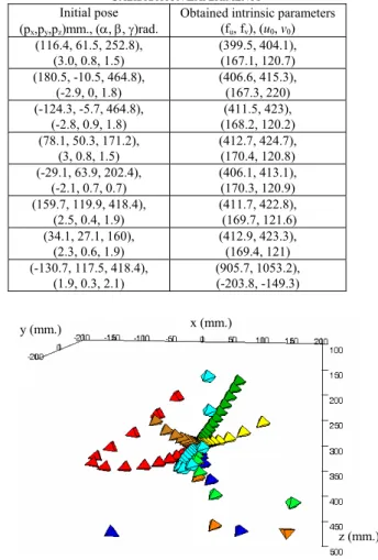
Once e = 0 the intrinsic and extrinsic parameters of the real camera are obtained. In Table I different calibration experiments using the VVS approach are shown. This table indicates the intrinsic parameters obtained (pixel coordinates of the principal point (u0, v0) and focal length in the u and v
directions (fu, fv)) from different initial positions of the
virtual camera. To develop the calibration the 3D object represented in Fig. 2 has been employed (from this object it is possible to extract 5 ellipses whose parameters have been used to define p and pd). The virtual trajectories obtained
during the different calibration experiments are represented in Fig. 1. The initial intrinsic parameters considered in the calibration are the ones provided by the manufacturer (u0,
v0) = (154, 99) and (fu, fv) = (313, 301). The real camera is
fixed at position (3.6, 39.7, 303.3) mm. and orientation in Euler angles (α, β, γ) = (2.9, 0.8, 1.5) rad. The intrinsic parameters obtained using the Zhang’s method [13] and a classical rig are (u0, v0) = (168.7, 121.5), and (fu, fv) =
(412.9, 423.7) respectively (20 images are used to do the calibration).
As is shown in Table I when VVS is employed for camera calibration, the intrinsic parameters obtained may vary depending on the initial view point. Furthermore, in Table I we can observe an experiment in which the obtained intrinsic parameters converge to wrong values due to a very bad initialization (see the last line). In order to avoid these errors the aspects described in Sections IV and V have been introduced in the basic VVS approach.
TABLE I
INTRINSIC PARAMETERS OBTAINED IN DIFFERENT MONO IMAGE
CALIBRATION EXPERIMENTS
Initial pose
(px,py,pz)mm., (α, β, γ)rad. Obtained intrinsic parameters (fu, fv), (u0, v0) (116.4, 61.5, 252.8), (3.0, 0.8, 1.5) (399.5, 404.1), (167.1, 120.7) (180.5, -10.5, 464.8), (-2.9, 0, 1.8) (406.6, 415.3), (167.3, 220) (-124.3, -5.7, 464.8), (-2.8, 0.9, 1.8) (411.5, 423), (168.2, 120.2) (78.1, 50.3, 171.2), (3, 0.8, 1.5) (412.7, 424.7), (170.4, 120.8) (-29.1, 63.9, 202.4), (-2.1, 0.7, 0.7) (406.1, 413.1), (170.3, 120.9) (159.7, 119.9, 418.4), (2.5, 0.4, 1.9) (411.7, 422.8), (169.7, 121.6) (34.1, 27.1, 160), (2.3, 0.6, 1.9) (412.9, 423.3), (169.4, 121) (-130.7, 117.5, 418.4), (1.9, 0.3, 2.1) (905.7, 1053.2), (-203.8, -149.3)
Fig. 1. 3D trajectories in different calibration experiments.
Fig. 2. 3D object employed in the camera calibration experiments.
III.COMBINING VISUAL SERVOING AND VIRTUAL VISUAL
SERVOING
In this section the main considerations and notations about the VS scheme developed jointly with VVS are detailed. A robotic task can be described by a function which must be regulated to 0. Such an error function et can
be defined as:
where s is a k x 1 vector containing k visual features corresponding to the current state, while s* denotes the
p = e& H v (4) ξϑ ⎛ ⎞ = ⎜ ⎟ ⎝ ⎠ v v & , p p ξ ⎛ ∂ ⎞ = ⎜ ∂ ⎟ ⎝ ⎠ p H L (5) 1 p λ + = v - H e (6) * t = -e s s (7) y (mm.) x (mm.) z (mm.)
visual features values in the desired state. s* depends not
only on the desired camera location,c od
M , but also on the
intrinsic parameters,ξ . A simple control law can be defined in order to fulfil the task et. By imposing an exponential
decrease of et (e&t = −λ2 te ), we obtain:
where + S ˆ
L is the pseudoinverse of an approximation of the
interaction matrix. In the estimation of the interaction matrix, ˆLs, the results of the calibration method described in the previous section are used.
Therefore, at each iteration, i, of the VS task, a complete VVS is developed. In VVS the desired features, pd, are the
ones observed at instant i (pd=s). The initial ones, p, are
computed by projection employing the extrinsic and intrinsic parameters determined at instant i-1. At each iteration of the VS task, the calibration results are used to update ˆLs and s*.
IV.MULTI-IMAGE CALIBRATION
As shown in [8] a possibility to improve the behaviour of classical VVS systems is to integrate data from several images. In this section, we present how to use different images obtained during the VS task. First we consider that the last w captured images are used. This set of w images is called calibration window. We consider that the intrinsic parameters do not vary or that in the w images the variation of the intrinsic parameters can be considered negligible.
The global matrix considered for the multi image calibration is then:
In this case, the control action and error in Equation (6) are
(
ϑ1, ϑ2, , ϑw,ξ)
=
v v v L v & , e=
(
p1−p p1d, 2−pd2, ,Lpw−pdw)
respectively. Therefore, in the minimization w virtual cameras are considered. A unique set of intrinsic parameters are computed which are the same for all the virtual cameras.
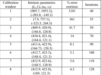
An important aspect of the multi image calibration is that it allows the convergence in situations in which mono image calibration cannot provide the correct intrinsic parameters. To demonstrate this fact, we consider the last experiment presented in Table I and the size of the calibration window is increased. Table II shows the intrinsic parameters obtained and the number of iterations required for the convergence depending on the size of the calibration window. This table also presents the percentage of error on
the extrinsic parameters obtained (this value includes the position but not the orientation). In this table we can see that the greater the calibration window the more iterations are required for the convergence, however, the calibration is more accurate. Furthermore, the use of a very high number of images for the calibration introduces delays and does not allow improvements of the value of the intrinsic parameters, when they vary during the task. From this table it is possible to conclude that it is required the size 6 of the calibration window to obtain good results.
TABLE II
EFFECT OF INCREASING THE NUMBER OF IMAGES TO DEVELOP THE
CALIBRATION Calibration window Intrinsic parameters (fu, fv), (u0, v0) % error extrinsic Iterations 1 (905.7, 1053.2), (-203.8, -149.3) 3181 40 2 (7.9, 757.1), (-523.5, 204.5) 561 55 3 (409.9, 420.9), (166.8, 120.8) 41.7 50 4 (410.4, 421.4), (164.4, 121.1) 14 70 5 (411.6, 422.9), (166.73, 120.3) 8.1 90 6 (412.7, 423.3), (168.4, 121.3) 3.1 100 7 (412.9, 423.6), (168.5, 120.9) 3.6 110 8 (412.9, 423.8), (169, 121.5) 4.2 120
V.CALIBRATION USING A VARIABLE NUMBER OF IMAGES
In this section a method to automatically determine the size of the calibration window is described. During the VS task a low number of images is adequate to reduce the required time processing. However, the use of a very small number of images could produce abrupt changes in the intrinsic parameters. Therefore, a variable number of images is the more adequate approach during the task. During the VS task different estimations of the intrinsic parameters are obtained. A Kalman filter is applied in order to estimate the correct value of the calibration parameters. The vector state
xk is composed by the intrinsic parameters, ξ, the extrinsic
parameters ( c o
M also represented here as r ) and its k
velocity r& . The process and measurement model are: k k +1 = k+ k
x Fx Gv (10)
k = k+ k
z Hx w (11)
where vk is a zero-mean white acceleration sequence and k
w is the measurement noise. Considering the velocity
model defined in (8), Equation (10) is given by:
(
)
2 k k +1 * k +1 2 s k k +1 k t 1 t 0 2 ˆ 0 1 0 λ t 0 0 1 0 ξ ξ ⎡Δ ⎤ ⎢ ⎥ ⎡ ⎤ Δ ⎡ ⎤ ⎡ ⎤ ⎢ ⎥ ⎢ ⎥ ⎢ ⎥ ⎢= ⎥ − − + Δ⎢ ⎥ ⎢ ⎥ ⎢ ⎥ ⎢ ⎥ ⎢ ⎥ ⎢ ⎥ ⎢ ⎥ ⎢ ⎥ ⎣ ⎦ ⎣ ⎦ ⎣ ⎦ ⎢ ⎥ ⎢ ⎥ ⎣ ⎦ + r r r& L s s v (12)(
*)
c= λ− 2ˆs − + v L s s (8) 1 p1 2 p2 p w pw 0 0 0 0 0 0 ξ ξ ξ ⎛ ∂ ⎞ ⎜ ∂ ⎟ ⎜ ⎟ ⎜ ∂ ⎟ ⎜ ⎟ =⎜ ∂ ⎟ ⎜ ⎟ ⎜ ⎟ ⎜ ∂ ⎟ ⎜ ∂ ⎟ ⎝ ⎠ p L p L H p L L L M M M L (9)and: 1 0 0 0 0 1 ⎡ ⎤ = ⎢ ⎥ ⎣ ⎦ H (13)
We have then considered the Generalized Likelihood Ratio (GLR) [12] to detect variations in the intrinsic parameters. To update the estimation of the state vector the following compensation equation is used:
(
)
(
) (
)
k +1 k +1 k +1 k +1 k +1 n k +1 o k;θ k;θ k;θ ξ ξ ⎡ ⎤ ⎡ ⎤ ⎢ ⎥ =⎢ ⎥ + ⋅ ⋅ ⎢ ⎥ ⎢ ⎥ ⎢ ⎥ ⎢ ⎥ ⎣ ⎦ ⎣ ⎦ r r r& r& a F -a j (14)where the sub-index n and o refers to the new and original state vectors, a
(
k;θ)
is the amplitude of the step obtained using the GLR algorithm, F is defined in (10) and(
k;θ) (
⋅ k;θ)
a j is the effect (on the value of the estimation
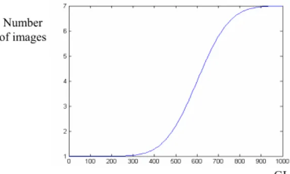
of the state vector measured at the iteration k) of the step that is produced at the iteration θ. This method is applied to detect changes in the camera intrinsic parameters. Therefore, only the last component of the vector state is updated in (14). Details of the implementation of the GLR can be seen in [10]. On the one hand, when GLR increases, the size of the calibration window is also increased in order to correctly estimate the value of the intrinsic parameters. On the other hand, if the GLR decreases, we consider that the system has correctly converged to the real intrinsic parameters and we decrease the size of the calibration window in order to improve the behaviour of the system (reducing delays).In order to implement this algorithm, the function represented in Fig. 3 has been defined to obtain the number of images of the calibration window depending on the value of the GLR.
VI.RESULTS
In this section, different tests that show the behaviour of the proposed adaptive VS system are described.
A. Problems in mono image calibration
With respect to the calibration convergence, VVS is able to converge when very large errors appear in the initialization. However, the obtained intrinsic parameters may be wrong depending on the initial extrinsic parameters due to local minima (see Table I). Considering the last experiment in Table I, once the VVS task ends, the obtained intrinsic parameters are: (u0, v0) = (-203.8, -149.3) and (fu,
fv) = (905.7, 1053.2). The extrinsic parameters obtained are:
position (-307.2 -250.7 -800.5)mm. and orientation in Euler angles (α, β, γ) = (2.9, 0.4, -1.8) rad. These values are far from the real intrinsic and extrinsic parameters (see Section II). In Fig. 4 and Fig. 5 the evolution of the mean error and intrinsic parameters is represented. In these figures we can see that aberrant values are obtained during the VVS task (see e.g. intrinsic parameters at iteration 7). At this moment the VVS should stop on a failure. However, in order to show the intrinsic parameters obtained during this experiment, more iterations are represented. This convergence problem
also appears in classical image-based visual servoing systems due to the camera retreat problem or local minima (see [1]). The camera trajectory during the task is also represented in Fig. 6.
Fig. 3. Function used to determine the number of images from the GLR.
Fig. 4. Mean error in pixel. Test 1.
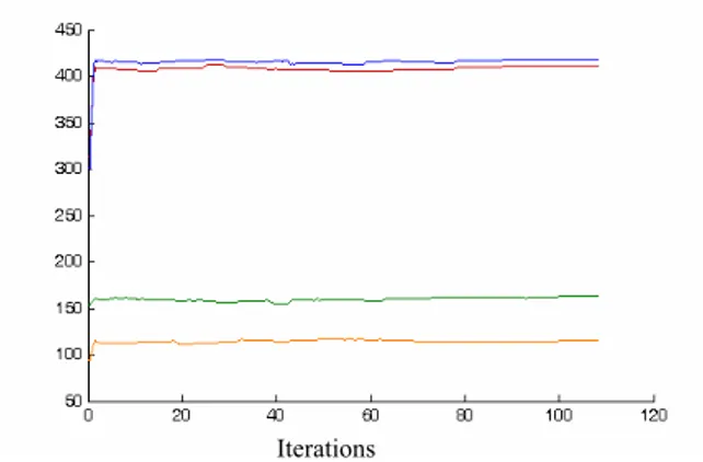
Fig. 5. Evolution of the intrinsic parameters. Test 1.
Fig. 6. Camera trajectory. Test 1.
B. Multi-image Calibration.
In order to illustrate the correct convergence of the multi image calibration in situations in which the mono image does not work correctly a detail of the convergence with 6 images is presented (see Table II). In this experiment the initial extrinsic and intrinsic parameters employed in test
Iterations Mean error (pix) Iterations x (mm.) y (mm.) z (mm.) Number of images GLR
1 are used. We have obtained the error and intrinsic parameters evolution shown in Fig. 7 and Fig. 8 respectively. The obtained intrinsic parameters are: (u0, v0) =
(168.4, 121.3) and the focal length equal to (412.7, 423.3). These values are very close to the ones obtained using previous existing methods (see camera calibration using the Zhang’s method in Section II). However, the convergence velocity has been decreased. The virtual camera trajectory during the task is also represented in Fig. 9.
Fig. 7. Mean error in pixel. Test 2.
Fig. 8. Evolution of the intrinsic parameters. Test 2.
Fig. 9. Camera trajectory. Test 2.
C. Adaptive Visual Servoing. Variable Number of Images.
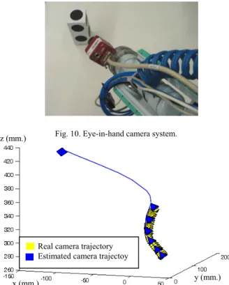
Now, we consider again the same initial intrinsic and extrinsic parameters but the eye-in-hand camera is tracking the trajectory shown in Fig. 11 during the VS task (real camera trajectory). To do so, the camera is mounted at the end-effector of a Mitsubishi PA-10 robot (see Fig. 10). At
each iteration of the VS task a complete convergence of the VVS is applied. Doing so, Fig. 11 represents a sampling of the estimated camera trajectory. Fig. 12 and Fig. 13 show the evolution of the error and intrinsic parameters when variable number of images is considered in the multi image calibration. The obtained intrinsic parameters are: (u0, v0) =
(168.8, 121.5) and the focal length equal to (413, 423.9). Once the VS is achieved we have obtained a mean error of 0,4mm in the determination of the extrinsic parameters (the real extrinsic parameters are the ones obtained using a classical camera calibration method executed at the final pose of the desired trajectory [13]). With respect to the previous test we can observe that a more accurate calibration is obtained. At each iteration of the VS task a complete convergence of the VVS is developed, therefore, at each iteration a more accurate calibration is obtained. During the first iterations the calibration window is progressively increased. From the fourth iteration the system obtains intrinsic parameters near to the real ones (see Figure 13). At this moment, the calibration window is quickly reduced to 1.
Fig. 10. Eye-in-hand camera system.
Fig. 11. Camera trajectory during the VS task. Test 3.
Fig. 12. Mean error in pixel. Test 3. Iterations
Mean error (pix) Iterations
Iterations Mean error (pix)
x (mm.) y (mm.) z (mm.)
z (mm.)
x (mm.) y (mm.)
Real camera trajectory Estimated camera trajectoy
Fig. 13. Evolution of the intrinsic parameters. Test 3.
D. Visual Servoing using varying intrinsic parameters.
Finally an experiment in which the intrinsic parameters vary during the task is presented. In this case, the robot is carrying out the VS task described is previous section. However, during the task the camera zoom varies. A camera calibration has been performed using the Zhang’s method [13] obtaining: (u0, v0) = (156, 124.8) and (fu, fv) = (526.5,
539.8). These values are the initial ones considered by the VVS. In Fig. 14 and Fig. 15 the intrinsic parameters and the size of the calibration window evolution is represented. Once the VS task ends the intrinsic parameters obtained are: (u0, v0) = (155.5, 125) and (fu, fv) = (944.9, 966.8)
(calibrating the camera at the end of the VS task using the Zhang’s method, the intrinsic parameters obtained are: (u0,
v0) = (156.2, 124.7) and (fu, fv) = (945.4, 967.3)). The
system is thus able to correctly determine the value of the focal length when it varies during the task.
Fig. 14. Evolution of the intrinsic parameters. Test 4.
Fig. 15. Evolution of the size of the calibration window. Test 4.
VII.CONCLUSIONS
We have presented in this paper a method to estimate the camera calibration parameters during a visual servoing task. With only one image, the calibration parameters estimated may differ depending on the initial extrinsic parameters and may be far from the real ones. Multi image calibration increases the robustness of the system. However, in this last approach an important issue is the determination of the size of the calibration window. Greater the calibration window is, more accurate the calibration will be. However, more iterations are required for the convergence of the system. In order to automatically determine the size of the calibration windows an approach based on the GLR has been proposed. It allows the correct convergence of the system with less iterations, and with a less oscillating behaviour.
This type of adaptive VS systems has been validated in situations in which the intrinsic parameters vary during the task. Furthermore, at each moment, the system is also able to estimate the camera pose.
REFERENCES
[1] F. Chaumette. “Potential problems of stability and convergence in image-based and position-based visual servoing”. In The Confluence
of Vision and Control, D. Kriegman, G . Hager, A.S. Morse (eds.),
LNCIS Series, No 237, pp. 66-78, Springer-Verlag, 1998.
[2] A.I. Comport, E. Marchand, M. Pressigout, and F. Chaumette. “Real-time markerless tracking for augmented reality: the virtual visual servoing framework,” IEEE Trans. on Visualization and Computer
Graphics, vol. 12, no. 4, pp. 615-628, July 2006.
[3] B. Espiau, F. Chaumette, and P. Rives, “A new approach to VS in robotics,” IEEE Trans. on Robotics and Automation, vol. 8, no 6, pp. 313-326. June 1992.
[4] E. E. Hemayed. “A survey of camera self-calibration,” in Proc. IEEE
Conference on Advanced Video and Signal Based Surveillance,
Miami, USA, 2003, pp. 351 – 357.
[5] S. Hutchinson, G. D. Hager, and P. I. Corke, “A tutorial on visual servo control”, IEEE Trans. Robotics and Automation, vol. 12, no. 5, pp. 651-670, Oct. 1996.
[6] K. Kinoshita, K. Deguschi, “Simultaneous determination of camera pose and intrinsic parameters by visual servoing”, in Proc. 12th International Conference on Pattern Recognition, Jerusalem, Israel, vol. A, 1994, pp. 285-289.
[7] E. Malis “Visual servoing invariant to changes in camera intrinsic parameters,” IEEE Transaction on Robotics and Automation, vol. 20, no. 1, pp. 72-81, Feb. 2004.
[8] E. Marchand and F. Chaumette. “A new formulation for non-linear camera calibration using VVS”. Publication Interne 1366. IRISA. Rennes, France. 2001.
[9] E. Marchand and F. Chaumette. “Virtual visual servoing: a framework for real-time augmented reality”, in Proc. Eurographics 2002, Saarebrücken, Germany, 2002, vol. 21, no. 3, pp. 289-298.
[10] J. Pomares and F. Torres, “Movement-flow based visual servoing and force control fusion for manipulation tasks in unstructured environments,” IEEE Transactions on Systems, Man, and
Cybernetics—Part C, vol. 35, no. 1, pp. 4 – 15. Jan. 2005.
[11] R. Y. Tsai, “A versatile camera calibration technique for high accuracy 3D machine vision metrology using off-the-shelf TV cameras and lenses,” IEEE J. Robotics Automat., vol. RA-3, no. 4, pp. 323-344, 1987.
[12] A. S. Willsky and H. L. Jones. “A generalized likelihood ratio approach to the detection and estimation of jumps in linear systems,”
IEEE Trans. Automat. Contr., vol. 21, no. 1, pp. 108-112. 1976.
[13] Z. Zhang. “Flexible camera calibration by viewing a plane from unknown orientations,” in International Conference on Computer
Vision, Corfu, Greece, 1999, pp. 666-673.
Iterations Iterations Iterations Number of images