D7.3 Report on simulator test results and driver acceptance of PROSPECT functions

HAL Id: hal-02264013

https://hal.archives-ouvertes.fr/hal-02264013

HAL is a multi-disciplinary open access

archive for the deposit and dissemination of sci-entific research documents, whether they are pub-lished or not. The documents may come from teaching and research institutions in France or abroad, or from public or private research centers.

L’archive ouverte pluridisciplinaire HAL, est destinée au dépôt et à la diffusion de documents scientifiques de niveau recherche, publiés ou non, émanant des établissements d’enseignement et de recherche français ou étrangers, des laboratoires publics ou privés.

Niklas Strand, Bruno Augusto, Irene Gohl, Johann Stoll, Pablo Puente

Guillen, Marie-Pierre Bruyas, Marie Jaussein, Evan Gallouin, Klaus Perlet,

Mats Petersson, et al.

To cite this version:

Niklas Strand, Bruno Augusto, Irene Gohl, Johann Stoll, Pablo Puente Guillen, et al.. D7.3 Report on simulator test results and driver acceptance of PROSPECT functions. [Research Report] IFSTTAR - Institut Français des Sciences et Technologies des Transports, de l’Aménagement et des Réseaux. 2018, 99 p. �hal-02264013�

EUROPEAN COMMISSION

EIGHTH FRAMEWORK PROGRAMME

HORIZON 2020

Page | 1 out of 98 The research leading to the results of this work has received funding from the European Community's Eighth Framework Program (Horizon2020) under grant agreement n° 634149.

Deliverable No. D7.3

Deliverable Title Report on simulator test results and driver acceptance of PROSPECT functions

Dissemination level Public Dd/mm/yyyy

Written by

Strand, Niklas VTI

Augusto, Bruno VTI

Gohl, Irene AUDI AG

Stoll, Johann AUDI AG

Puente Guillen, Pablo TME

Bruyas, Marie-Pierre IFSTTAR

Jaussein, Marie IFSTTAR

Gallouin, Evan IFSTTAR

Perlet, Klaus BMW

Petersson, Mats VCC

Johansson, Regina VCC

Meltzer, Elin VCC

Ljung Aust, Mikael VCC

Braeutigam, Julia BAST

Large, David University of Nottingham

Checked by Last Name, Name Organisation Dd/mm/yyyy

Bánfi Miklós Gábor BME

Approved by Last Name, Name Organisation Dd/mm/yyyy

Page | 2 out of 98

E

The process of developing new automotive systems includes various testing cycles to assure a save operation in traffic. Physical system testing on test tracks is very important for this purpose, but rather expensive and might only become possible in later stages of the development process. Using a virtual simulation environment offers a safe possibility of testing new systems in early stages of development. Aditionally, driver-in-the-loop tests at test track and in a virtual simulator make it possible to evaluate driver reaction and potential acceptance by the future users of those systems. Within PROSPECT the new functions are investigated under various aspects in several simulator studies and test track studies.

This deliverable D7.3 gives detailed information of conduction and results of the each study. Three studies focus exclusively on the for Vulnerable Road Users (VRUs) specifically dangerous urban intersection scenarios. The first of those studies examines the driver behaviour in a turning situation when a byciclist might be crossing. The described phenomena are looked-but-failed-to-see and failed-to-look. The second study, which provides an initial step in this line of research, analyzed the acceptance of issued forward collision warning times. The positioning of the potential accident opponent and the subjective feeling towards the criticality of the situation by the driver were key parameters taken into account. Last, but not least the acceptance of an intersection assist autonomous emergency braking systems was tested regarding the acceptance of potential buyers. The study was run for five days in a row for each participant to be able to judge the behaviour in a comuting situation. Two studies focused on longitudinal scenarios. Both studies followed the same design, but one was conducted on a test track and the other one in a simulator. The main objective was to investigate drivers reactions to FCW warnings and Active Steering interventions in critical VRU scenarios in case of a distraction of the driver. Additionally, the test track study was used to validate the results from the simulator study.

The results of those studies are the basis for a wide acceptance evaluation of the systems. No system is an asset in increasing road safety if it is not accepted by the user and therefore turned off, if it is not required the system to be default on in consumer tests. Complemented by an additional acceptance study where the participants had to give their opinion of those systems after they watched videos of dangerous situations, the acceptance was analyzed based on questionnaires developed in PROSPECT and reported in Deliverable 7.2. This wholistic approach allows an expert discussion on the potentials of the PROSPECT functions in the future.

Page | 3 out of 98

C

3 Experiment #1 “Audi experiment t 7.2” ... 10

3.1 Theoretical background and focus of the study ...10

3.2 method ...13

3.2.1 Experimental design and driving tasks ... 13

3.2.2 Participants ... 15

3.2.3 Equipment and recorded data ... 15

3.2.4 Procedure ... 17 3.3 Results ...18 3.3.1 Data analysis ... 18 3.3.2 Subjective results ... 18 3.3.3 Objective results ... 21 3.4 Conclusions ...22

4 Experiment #2 “ Drivers’ Acceptance towards warnings based on driver models” ... 24

4.1 Methods ...24

4.1.1 Methodology ... 24

4.1.2 Test setup ... 24

4.1.3 Research design and scenario ... 25

4.1.4 Procedure ... 26

4.1.5 Participants ... 27

4.2 Results ...27

4.2.1 Brake onset after warning ... 27

4.2.2 Acceptance questionnaire ... 28

4.2.3 Correlation ... 31

4.3 Conclusions ...31

5 Experiment #3 “University of Nottingham Acceptance testing” ... 33

5.1 Overview ...33

5.1.1 Methodology ... 33

Page | 4 out of 98

5.2 Results ...36

5.2.1 Defining Criticality of Situation ... 36

5.2.2 Assessment of System Acceptability ... 36

5.2.3 Assessment of System Trust ... 37

5.2.4 Intention to Activate/Use Warning Function ... 38

5.2.5 Intention to Activate/Use Braking Function ... 38

5.2.6 Willingness to Buy A PROSPECT-Like System ... 39

5.3 Analysis ...40

5.4 Conclusions ...40

6 EXPERIMENT #4“DRIVER REACTION TO FCW WARNING AND AUTOMATIC STEERING INTERVENTION IN CRITICAL VRU SCENARIOS” ... 41

6.1 METHOD FOR SIMULATOR EXPERIMENT ...41

6.1.1 Research design ... 41 6.1.2 Participants ... 41 6.1.3 Materials ... 42 6.1.4 Performance indicators ... 45 6.1.5 Procedure ... 45 6.1.6 Analysis ... 46

6.2 METHOD FOR THE TEST TRACK EXPERIMENT ...46

6.2.1 Research Design ... 46

6.2.2 Participants ... 46

6.2.3 Equipment ... 47

6.2.4 Procedure ... 48

6.3 DATA ANALYSIS ...49

6.4 DIFFERENCES IN METHOD BETWEEN SIMULATOR AND TEST TRACK EXPERIMENTS ...50

6.4.1 Research Design ... 50

6.4.2 Methods ... 51

6.4.3 Procedure ... 51

6.5 RESULTS FROM PEDESTRIAN TESTS WITH FCW ONLY AT TEST TRACK AND IN SIMULATOR INCLUDING VALIDATION ...51

6.5.1 Gaze Reaction Times from Test Track ... 52

6.5.2 Reaction Types ... 52

6.5.3 Steering Reaction Times from Test Track and Sim IV ... 52

6.5.4 Braking in Sim IV and Test Track ... 53

6.5.5 Distance to Conflict Object in Sim IV and on Test Track ... 55

6.5.6 Collisions in Sim IV and on Test Track ... 58

6.6 RESULTS FROM PEDESTRIAN TESTS WITH FCW W/WO AUTOMATIC STEERING INTERVENTION AT TRACK TESTING ...58

6.6.1 Reaction Types ... 58

6.6.2 Steering Behaviour ... 59

6.6.3 Lateral Distance ... 60

6.7 RESULTS FROM CYCLIST TESTS WITH FCW W/WO AUTOMATIC STEERING INTERVENTION IN DRIVING SIMULATOR ...63

6.7.1 Steering behaviour ... 63

6.7.2 Severity ... 67

6.7.3 Acceptance evaluation ... 67

6.8 CONCLUSIONS ...71

Page | 5 out of 98

7.1 Global research design ...72

7.2 Participants ...72 7.3 Focus groups ...73 7.3.1 Procedure ... 73 7.3.2 Materials ... 74 7.3.3 Results ... 76 7.4 Video-based experiment ...80 7.4.1 Procedure ... 81 7.4.2 Materials ... 81 7.4.3 Results ... 83 7.5 Conclusions ...91

8 Discussion and Comparison of results ... 94

8.1 Method related aspects ...94

8.2 Overall Acceptability Evaluation ...94

9 References ... 96

Page | 6 out of 98

1 I

1.1 BACKGROUND

To test safety measures in real traffic may induce risks for drivers and therefore it is important to provide safe test environments with the human-in-the-loop, especially for early stage prototype systems. Such test environments can be set up in driving simulators or test tracks. A key to successful evaluation of active safety systems is to include the driver reaction and response to the system intervention to assure that the system itself does not impose any additional risks for the driver. Another important aspect for the evaluation is user acceptance. Without user acceptance the success of any active safety system is challenged. A low acceptance towards the system may lead to deactivating the system or not buying the system. Within PROSPECT, an acceptance methodology that can be used while evaluating active safety has been developed and used in the studies reported here.

1.1.1 Prospect

Recently active pedestrian safety systems with the capability of autonomous emergency braking (AEB-PED) in specific critical situations have been introduced to the market. Proactive Safety for Pedestrian and Cyclists (PROSPECT) is an EU funded project set out to improve the effectiveness of active safety systems targeting vulnerable road users (VRU). In PROSPECT there are two main targets to achieve this, namely: (1) by expanding the scope of the addressed scenarios, and (2) through improved overall system performance.

1.1.2 Deliverable outline

This deliverable addresses results from acceptance testing and testing of active safety measures on test tracks and in driving simulators. In the first chapter the background providing the rationale for conducting the tests are introduced followed by a brief introduction to the PROSPECT project and the objectives. In the second chapter the general methodology describing driving simulators, test tracks, and acceptance testing is described. Thereafter, each test and experiment is described in detail in their own chapters respectively. Following the chapters on each experiment, a chapter providing a discussion and a comparison of results is provided. In the last chapter of the deliverable the overall conclusions are provided.

Page | 7 out of 98

2 G

2.1 USE CASES

Twelve use cases have been identified within WP2 and WP3 to be implemented in the demonstrators: 9 for cyclists and 3 for pedestrians (Figure 1). Even reduced, this number still addresses around 80% of all cyclist accidents investigated in WP3. Behaviours such as the velocity, distance and offset of the vehicle and VRUs (cyclists and pedestrians) are defined in Deliverable D7.2 (Report on methodology for balancing user acceptance, robustness and performance). Scenarios can then be realized on the test tracks or in simulator environments. For each use case, storyboards describe what the demonstrators intend to do based on the situation analysis and the risk assessment. To do so, each use case is divided into three distinct scenario groups: Safe Scenario (S), Critical Scenario (C) and Possible Critical Scenario (PC). Information is provided in Deliverable D7.2 (Report on methodology for balancing user acceptance, robustness and performance).

UC with cyclists

UC with pedestrians

Figure 1: The 12 Demonstrator Use Cases defined within WP2 and WP3

A set of tests and experiments described in the current deliverable have been designed within T7.2 and T7.3 in order to evaluate the different PROSPECT systems. These tests were carried out in various contexts with the aim of covering most of the demonstrator use cases (Table 1) including pedestrians and cyclists and all functionalities of the PROSPECT systems.

Page | 8 out of 98 Table 1: Experiments carried out within T7.2 and T7.3.

2.2 DRIVING SIMULATORS

In PROSPECT driving simulator studies were used to identify and tune the user acceptance of proactive safety systems for vulnerable road users, as well as to test active safety functions in a controlled and repeatable environment. Furthermore, driving simulators provided a testbed to provide replicable human-in-the-loop tests of active safety systems with active braking and steering capacity at varying stages of system development. The use and value of driving simulators as a tool for development of active safety functions was thoroughly described by for instance Fischer, et al. (2011). Simulated mock-ups of active safety systems—including the human machine interface—resembling PROSPECT features were therefore implemented in different driving simulators across partners throughout Europe.

2.3 ACCEPTANCE METHODOLOGY

Acceptance testing is an important part of the project since it provides knowledge on the user perception of the proactive systems developed within PROSPECT. It is crucial for the success of such active safety systems that they are acceptable for the drivers (e.g. judged useful and trusted). If not, they could be permanently turned off and would then have no effect on traffic safety. Moreover, interventions of active systems being rare, they may lead to unpredictable reactions from non-aware drivers being potentially frightened or startled when activated.

Warning Braking Steering Possible critical scenario Critical scenario True positive False positive Audi /TME 5, 3 Cyclist X X X X X

VIL methodology & simulator expe.

UoN 2 Cyclist

Reversed (driving on the left)

X X X X X X Simulator experiment VTI /Volvo 12 Cyclist/ Pedestrian X X X X

Test track & Simulator expe.

2,4 Cyclist X X X X 10, 11 Pedestrian X X X X X Lab. expe. Focus groups Video IFSTTAR Activation Added description Partner UC N° VRU Use case pictogram

Page | 9 out of 98 In this context, a specific acceptance methodology was developed within Task 7.3. This methodology is described in Deliverable D7.2 (Report on methodology for balancing user acceptance, robustness and performance). It integrates acceptance of false positive (warnings and/or interventions occurring at inappropriate times) and false negatives (no warning or activation when needed) and evaluates their influence on the drivers’ acceptance.

Questionnaires are generally used to evaluate subjective components of constructs, such as acceptance and trust. The methodology is then based on existing questionnaires to be administered in tests and experiments that evaluate PROSPECT systems. By using common questionnaires, this work aims to enable an overall evaluation of the acceptance of the developed functions. Collecting them in such a way will ensure data is acquired in the same format and thus can easily be compared.

In the literature, acceptability is generally distinguished from acceptance. Acceptability is measured when the person has no experience of the system, as an “a priori measure of the extent to which a person thinks they will accept and use a system. Acceptance, on the other side, is determined after use and is a measure of how much a person actually uses a technology and the satisfaction with this experience”.

Three questionnaires are completed at different times of the tests:

- Before running the test/experiment: questionnaire 1 (participant information) and 3 (global expected acceptance of the system or a priori acceptability, based on the “Perceived usefulness”, and “Perceived satisfaction” questionnaire of Van der Laan et al. (1997) and the Trust questionnaire of Jian et al. (2000)).

- During the test/experiment: questionnaire 2 (feedback on each situation the participants are being faced with, based on the Risk Awareness measurement developed by Bellet and Banet, (2012)).

- After the test/experiment: questionnaire 3 (global acceptance of the system after having experienced it)

Before distributing the first questionnaire, the experimenter must give sufficient information about the functioning of the system to the participants. This information will allow the driver to gain some familiarity with the system and to create a mental model of what will be tested. The second acceptance questionnaire allows for measuring changes in acceptance as a result of the system experience.

The questionnaires have been developed with the objective to make acceptance evaluation not too invasive during the tests, and to disturb the test participants as little as possible. For that reason, the questionnaire completed during the experiment is very short. The two other questionnaires used before and after experiments could be longer as they do not interfere with the experiment.

Page | 10 out of 98

3 E

#1

“A

7.2”

3.1 THEORETICAL BACKGROUND AND FOCUS OF THE STUDY

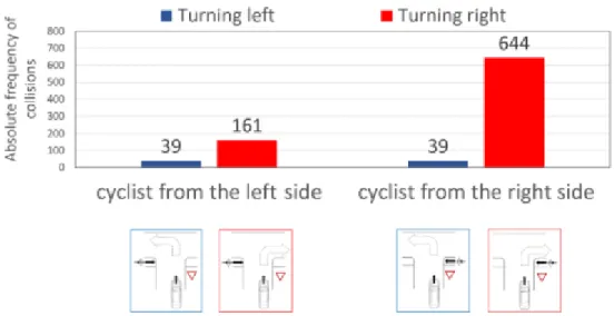
The output from task T2 defined the most relevant car-to-cyclist accident scenarios that should be addressed by next-generation VRU systems. Based on the results, the most relevant car-to-cyclist scenario is a driver approaching a non-signalized intersection or a T-junction and a cyclist crossing from a bicycle lane. In such situations the frequency to collide with a cyclist crossing from the right side is three times higher than with a cyclist crossing from the left side (Gohl, Schneider, Stoll, Wisch, & Nitsch, 2016). Furthermore, the frequency of collisions with a cyclist crossing from the right side as well as from the left side decreases when the driver’s maneuver intentions are taken into account. Figure 2 shows that left-turning drivers collided less frequently than right-turning drivers, irrespective of the orientation of the cyclist.

Figure 2: Absolute frequency of collisions depending on driver’s task and the crossing direction of the cyclist.

A general explanation why drivers turning right fail to manage situations with a cyclist from the right more often than drivers turning left is the drivers’ improper attention allocation strategies, as demonstrated by Summala et al. (1996). In unobtrusive field observations at T-junctions, Summala et al. (1996) studied drivers’ visual scanning strategy at left and right turns. The results showed that drivers‘ visual scanning patterns differentiate according to their task goals: drivers turning left tended to look in both directions, whereas drivers turning right rather continued to look left. According to the authors, these different scanning patterns implied an attentional bias towards conflicting motor vehicles due to drivers’ erroneous expectations. These expectations are formed by drivers’ practice, integrating the perceived environmental cues in a certain context and task into hierarchically organized schemata including both what potential hazards may occur and where they may appear (Engström, 2011). This knowledge-driven processes, called “top-down processes”, may lead to critical situations if the drivers‘ expectation does not match the actual situation. As a result, drivers turning right selectively looking for cars approaching from the left will

Page | 11 out of 98 probably fail to notice the cyclist coming from the right. In addition, the probability to notice the cyclist coming from the right is decreased for right-turning drivers when the traffic density from the left is high, as demonstrated by Werneke and Vollrath (2012). In contrast, drivers turning left have to yield for cars from both sides. Even if the left-turning driver did not account for cyclists from the right, the chance of the cyclist being able to attract attentional focus through reflexive bottom-up processes is higher than for right-turning drivers since the cyclist appeared within the drivers’ field of view (Summala & Räsänen, 2000).

Moreover, the latter provides an explanation why drivers turning right fail to manage situations with a cyclist from the right more often than with a cyclist from the left. As pointed out above, drivers turning right may fail to look in the direction of the cyclist crossing from the right, thus the cyclist appears entirely outside the drivers’ field of view. If the cyclist appears within the field of view (e.g. cyclist crossing from the left), bottom-up selection may prevent drivers from colliding with that cyclist and thus reduce the overall frequency of collisions.

However, drivers turning right still collide quite frequently with cyclists from the left (see ¡Error! No se encuentra el origen de la referencia.), though the chance of the cyclist being able to capture the driver’s attention is increased due to the bottom-up selection. One contributing factor to the reduced ability of cyclists to capture the drivers’ bottom-up processes within the drivers field of view is their poor sensory conspicuity, i.e. the degree of difficulty to perceive an object from its environment due to its physical characteristics such as size, brightness, illumination, color and movement (see e.g., Rogé, Ndiaye, Aillerie, Aillerie, Navarro, & Vienne, 2017; Tin Tin, Woodward, & Ameratunga, 2015). The results gained from task T2.1 support the hypothesis that poor sensory conspicuity may play a critical role in crash causation in such situations, as over a quarter of these accidents happened during nighttime or dawn (Gohl, Schneider, Stoll, Wisch, & Nitsch, 2016).

However, since most of these accidents happened during daytime, it may be assumed that drivers looked but failed to see the salient cyclist coming from the left appearing within their field of view. In the field of perceptual psychology this phenomenon is known as inattentional blindness (e.g., Mack and Rock, 1998; Simons and Chabris, 1999) and “refers to the inability to detect salient stimuli appearing in the field of view if attention is allocated elsewhere” (Engström, 2011, p.14). For instance, Simons and Chabris (1999) demonstrated in an experiment that this phenomenon is truly existing. While participants had to count the number of passes between basketball teams in a video clip, a person dressed as a black gorilla walked through the mass of players. After the study, about 30-70% of the participants (White and Caird, 2010) reported that they did not notice this very salient object in their direct field of view. In recent years, many studies including in-depth accident analyses, self-reported near accidents and experimental studies conducted in simulators investigated the looked-but-failed-to-see error in the driving context (e.g., Brown, 2005; Herslund & Jorgensen, 2003; Koustanai et al., 2008; Clarke et al., 2004; Mitsopoulos-Rubens and Lenné, 2012; Roge, 2011; Roge, 2017). The general consensus of these studies is that the looked-but-failed-to-see phenomenon may

Page | 12 out of 98 arise from the observers erroneous expectations of what they are likely to see, and as a consequence they might unintentionally filter out the unexpected or infrequent objects without perceiving them. As a result, the looked-but-failed-to-see error could be less pronounced for drivers who cycle regularly themselves, compared to drivers who never cycle, since the former are more aware of the presence of cyclists. In fact, as demonstrated recently by Roge et al. (2017), cyclists’ visibility depends on their cognitive conspicuity for car drivers rather than their sensory conspicuity. The authors concluded that attentional selection of a cyclist in the road environment during car driving depends mainly on top-down processing. But, as mentioned above, the results from T2.1 indicate that sensory conspicuity may be a contributing factor in such situations, in which a driver intends to turn right at a T-junction and a cyclist is crossing from the left. Top-down processes in terms of erroneous expectations of what kind of potential hazards may occur solely cannot explain the higher proportion of accidents that happened during nighttime or dawn.

Indeed, in natural driving situations, attention selection is typically the result of a dynamic interaction between both top-down and bottom-up selection. However, very little is known about this interaction and especially how and in which situations drivers bottom-up processes prevent them from colliding with cyclists when turning right at T-junctions even if drivers do not account for cyclists at all. Based on the literature above, it may be assumed that erroneous expectations will decrease drivers’ ability to detect cyclists from both sides. If the visibility of cyclists depends on their cognitive conspicuity for car drivers, the car drivers who are aware of cyclists would avoid more collisions and would detect cyclists earlier than car drivers who do not account for cyclists. Since it was shown that drivers erroneous expectations lead to an attentional bias towards car objects (Summala, Pasanen, Räsänen, & Sievänen, 1996) resulting in a visual scanning behaviour biased to the left leg of the intersection, the probability to detect the cyclists from the left is higher than cyclists from the right, irrespective of the sensory conspicuity.

Moreover, if drivers’ visual behaviour when turning right is biased towards car objects from the left, then cyclists who are coming from the right side will not be able to attract the drivers attention even if the cyclists sensory conspicuity is high. Therefore, drivers would show an equal detection performance of cyclists from the right side, regardless of the cyclists sensory conspicuity. In contrast, the results from T2.1 indicate that the ability to interrupt the drivers biased visual behaviour towards cyclists crossing from the left side depends on their sensory conspicuity. Therefore, it is hypothesized that drivers would show a better detection performance of cyclists from the left side with high sensory conspicuity compared to those with lower sensory conspicuity.

In addition, as demonstrated by Werneke et al. (2012), the extent of attentional bias towards the left side depends on traffic density from the left side. As a result, it may be assumed that in situations where no other objects (e.g. cars) from the left side appear, drivers would show a better detection performance of cyclists.

Page | 13 out of 98

3.2 METHOD

3.2.1 Experimental design and driving tasks

In order to examine how and in which situations the drivers bottom-up processes prevent them from colliding with cyclists when turning right at T-junctions - especially if drivers do not account for cyclists - three situational factors were varied.

At first, two T-junction scenarios were randomized with either crossing traffic or without crossing traffic. Both T-junctions presented a yield sign indicating that the drivers had to give way. In the scenario with crossing traffic, one black and one red car were placed on the left side of the main road of the T-junction at a distance of 72 m and 30 m, respectively. When participants approached the T-junction, the red car started to cross the intersection with a mean velocity of 50 km/h from the left to the right once the relative temporal distance fell below 10 seconds. In contrast, the black car remained in its initial position. Both cars indicated to the participants that there would be some traffic at this T-junction. At the second T-junction there was no crossing or parked traffic at all.

Moreover, the crossing direction of the cyclist was varied between crossing from the left and crossing from the right side. Every cyclist was positioned at a distance of 53 m from the middle of the T-junction. When participants approached the T-junction, the cyclist started to cross the intersection with a mean velocity of 20 km/h once the participant reached a distance of 75 meters from the middle of the T-junction. To obtain comparable results, both T-junctions had the same geometry, so that the cyclist becomes visible at the same time, regardless of his crossing direction.

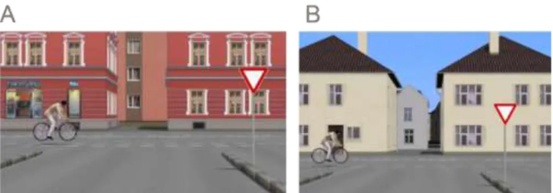
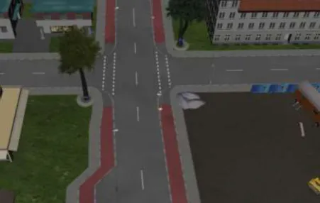
Since bottom-up processes are directly affected by the sensory conspicuity of an object, two different levels of cyclist’s sensory conspicuity were selected as independent variable: low and high sensory conspicuity. In the high sensory conspicuity scenario, the cyclist was dressed in white and appeared against a colored background (see Figure 3 A). In contrast, in the low sensory conspicuity scenario the cyclist was also dressed in white but appeared against a similarly colored background (see Figure 3 B).

Figure 3: Levels of cyclist’s sensory conspicuity varied within the study: high (A) and low (B) sensory conspicuity.

Page | 14 out of 98 Since it is known that erroneous expectations will influence drivers’ gaze and driving behaviourbehaviour which decreases the drivers ability to detect cyclists, several rounds without crossing cyclists were needed to build up erroneous expectations of what potential hazards may occur, i.e. decrease the participants expectation of a cyclist crossing. In order to compare drivers’ gaze behaviourbehaviour with and without additional crossing traffic in non-critical situations (baseline-condition), each participant was confronted with both T-junctions, the one with the additional crossing traffic and the one without additional crossing traffic (within-subject design). Once participants completed two trials without crossing cyclists, they were confronted with a crossing cyclist at the next T-junction in a third trial. It may be assumed that this unexpected encounter with a cyclist will sensitize the participants to the presence of cyclists, resulting in a more alert gaze and driving behaviourbehaviour. To ensure that participants are unaware of cyclists in all encounters, each participant can be tested only once in a critical incident. As a result, for all three situational factors varied within this experiment a between-subjects design in encounter situations was used (see Figure 4).

Figure 4: The resulting experimental design in encounter situations.

Although it is known that erroneous expectations will decrease the driver’s ability to detect cyclists, the inverse conclusion is uncertain. Therefore, the hypothesis of whether or not expectations which take cyclists into account will increase the drivers ability to detect cyclists (regardless of the cyclists sensory conspicuity, crossing direction and the presence/absence of additional crossing traffic) will be tested. For this purpose, each participant was faced a second time with a crossing cyclist at the second T-junction.

Page | 15 out of 98 Furthermore, the drivers’ gaze behaviourbehaviour was recorded with a head-mounted eye-tracking system (Eye Tracking Glasses 2 from SMI) in order to assess the drivers detection performance. As a result of using a head-mounted eye-tracking system, participants are fully aware that their eye movements will be recorded. This knowledge may unconsciously bias the participants gaze behaviourbehaviour. To dissuade participants from thinking that they have to behave in an exemplary manner (as obtaining their driver’s license), a cover story was constructed. The participants were instructed that the aim of the study was to examine which gaze parameters are suitable to predict the state of “mind wandering”. In order to ensure that all participants understand the term in the same way, the following definition was introduced: “Mind wandering is a state where the thought processes that occupy the mind are on topics that are unrelated to the task(s) at hand” (Yanko & Spalek, 2013, p. 81) [and are often experienced by drivers that after these periods] “they can hardly remember any of specifics associated with the drive” (Yanko & Spalek, 2013, p. 81). Consequently, the main driving task of the participants was to drive a defined route several times and whenever they experienced mind wandering, they had to flash the vehicle headlight.

3.2.2 Participants

The study consisted of a sample of 92 participants, of whom 31 were female and 61 male. The participants’ ages ranged from 19 to 56 years, with a mean age of M=29.5 years (SD=8.5 years). On average, participants obtained their driving license 12.2 years ago (SD=10.8 years). All participants requiring visual aid had to wear corrective contact lenses during the study in order to avoid interferences with the eyetracking system from SMI (Eye Tracking Glasses 2). The assignment of the participants to one out of eight groups was performed on the basis of their age, gender and average mileage per year.

3.2.3 Equipment and recorded data

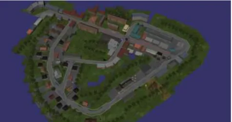
The test was performed in the driving simulator described in section 2.1. The simulated environment was created using the tool-chain VTD for driving simulation applications. The road environment included houses, stores, signs, sidewalks, cycle paths and oncoming car traffic besides the two junctions of interest. Two T-junctions and five intersections are embedded within this environment and are located as shown in Figure 5

Page | 16 out of 98 For each of the eight experimental design groups (see ¡Error! No se encuentra el origen de la referencia.), three driving scenarios were created (24 driving scenarios in total). The first scenario was used to become familiar with the simulator and the route. During this scenario the investigator was seated in the rear seat and pointed the way. The second scenario was identical to the first and was used to build up erroneous expectations of potential hazards. In contrast to the first, the investigator was sitting outside the car this time. The third scenario included the crossing cyclist at both T-junctions. Each of the three driving scenarios took 8-10 minutes to complete.

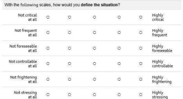
In this study, driving data, gaze behaviour and subjective data were recorded. Driving data, speed, longitudinal acceleration, actuation of the turn indicator, remaining distance to both T-junctions and a binary variable, which displays whether or not the driver collided with the cyclist in the last driving scenario, were recorded by the ADTF software. Besides the driving data, eye-tracking information was collected with Eye Tracking Glasses 2 from SMI. The gaze information was recorded at a 60 Hz rate. Both datasets, vehicle and eye-tracking data, were synchronized based on a time marker (participant activating the turn indicator while directing the gaze in the same direction). Regarding subjective data, participants received three questionnaires within this study. The first was used to collect general information about the participants such as age, driving experience (mean mileage per year, years of possession of driver’s license) and driving habits (frequency of car use, percentage distribution of driving time per road type including highway, rural and urban road). In the second questionnaire participants evaluated their perception of the driving situation after the first encounter with a crossing cyclist using the dimensions of the second questionnaire proposed in Deliverable D7.2. But instead of the continuous scales, participants had to indicate their level of agreement on 5-point Likert scales (see Figure 6).

Page | 17 out of 98 Figure 6: Evaluation of participants’ perception of the driving situation after the first encounter with a crossing cyclist.

Moreover, some questions were added concerning whether or not the driver has seen the cyclist in time and whether or not the driver has foreseen that a cyclist would cross at this T-junction. The third questionnaire was administered to measure changes in the drivers perception of the driving situation as a result of the increased awareness of cyclists. In addition, the participants were queried on a 5-point Likert scale whether they would like a driver assistance system in these situations. Finally, participants received some questions concerning their cycling habits (frequency of cycle use, usage of the cycle path against driving direction).

3.2.4 Procedure

After reading the brief instructions, the participants filled out the first questionnaire concerning their demographic characteristics and driving experience. Based on their age and mileages per year, participants were assigned to one of the eight experimental groups. Once the participants adjusted the seat and steering wheel of the car, the eye-tracking system was put on and the calibration was carried out. Subsequently, the participants were driving the first two driving scenarios without a crossing cyclist. There was a short break after both driving scenarios. After the second break, they drove the scenario a third time, but this time there was a crossing cyclist at both T-junctions. Between the two encounter situations the participants had to evaluate the situation with the second questionnaire. Shortly after the second encounter, they stopped a last time and filled out the third questionnaire. The procedure is summarized in Figure 7. The whole experiment for each participant lasted about 45 minutes.

Page | 18 out of 98 Figure 7: Experimental procedure in the driving simulator study.

3.3 RESULTS

3.3.1 Data analysis

The results presented here focus on the participants subjective perception of the driving situation as well as the participants objective detection performance in the first critical encounter with a crossing cyclist.

For data analysis the statistical software SPSS 24 was used. In order to describe the influence of the cyclists sensory conspicuity, the cyclists crossing direction and the presence or absence of additional crossing traffic on the evaluation of driver’s perception of the driving situation with a crossing cyclist, a 2 (cyclist’s sensory conspicuity) x 2 (cyclist’s crossing direction) x 2 (additional crossing traffic) univariate ANOVA was conducted for each scale.

With regard to the analysis of driver’s objective detection performance, a measurable parameter for the drivers detection performance needs to be defined. Therefore, in a first step for each driver, the moment at which s/he moves her/his gaze towards the cyclist was identified. This moment can be expressed in meters and represents the relative distance that is left before the bicycle path is reached. In order to account for different approaching velocities, the subject’s relative distance was then divided by his/her velocity at this moment and represents the time left to react to the cyclist. Finally, a 2x2x2 univariate ANOVA was performed.

3.3.2 Subjective results

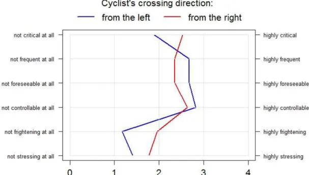
With regard to the criticality scale, the 2x2x2 ANOVA revealed a significant main effect only on the cyclists crossing direction (F(1,87)=6.284, p=.014, ηp²=.067). The effect of cyclist’s sensory conspicuity, additional crossing traffic and the interaction effects were not significant. As Figure 8 shows, the participants experienced the driving situation with a crossing cyclist from the right (M=1.89, SE=.179) as more critical than the driving situation with a crossing cyclist from the left (M=2.52, SE=.176).

With regard to driver’s perception of the frequency of the experienced driving situation in real world, the ANOVA showed no significant main or interaction effects. Nevertheless, there is a marginal significant main effect of cyclist’s crossing direction (F(1,87)=3.481, p=.065, ηp²=.038). Participants reported that they experienced the driving situation with a crossing cyclist from the left (M=2.69, SE=.144) more

Page | 19 out of 98 frequently than the driving situation with a crossing cyclist from the right (M=2.31, SE=.142) (see Figure 8).

Figure 8: Participants’ evaluation of the driving situation depending on cyclist’s crossing direction.

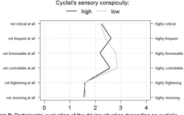
With regard to the foreseeability of a driving situation, the ANOVA showed a significant main effect of the cyclists sensory conspicuity (F(1,87)=11.036, p=.001, ηp²=.113). Interestingly, as shown in ¡Error! No se encuentra el origen de la referencia., participants reported that the driving situation with a crossing cyclist of low conspicuity (M=2.77, SE=.127) is more foreseeable than the driving situation with a crossing cyclist of high conspicuity (M=2.16, SE=.132). The remaining effects were not significant.

Page | 20 out of 98

Figure 9: Participants’ evaluation of the driving situation depending on cyclist’s

sensory conspicuity.

Regarding the controllability of a driving situation, the ANOVA revealed no significant main or interaction effect. However, there is a marginal interaction effect between the cyclists crossing direction and additional traffic (F(1,87)=2.911, p=.092, ηp²=.032). As shown in Table 2, participants rated the driving situation with a crossing cyclist from the right more controllable when there was no additional traffic from the left side as compared to that with additional traffic. For driving situations with a crossing cyclist from the left, the opposite effect was found. Participants perceived this situation more controllable when there was additional traffic from the left side as compared to the driving situation without additional traffic.

Table 2: Perceived controllability of the driving situation depending on cyclist’s crossing direction and additional traffic.

Cyclist’s crossing direction from the left from the right Additional traffic

from the left side

yes 2.913s ( SE=.216) 2.417s ( SE=.211) no 2.689s ( SE=.212) 2.917s ( SE=.211) With regard to the participants evaluation of how frightening the driving situation was, the ANOVA showed a significant main effect of the cyclists crossing direction (F(1,87)=11.269, p=.001, ηp²=.115). With a mean value of 1.19 (SE=.172), participants reported a lower fright when the cyclist is crossing from the left side

Page | 21 out of 98 compared to when the cyclist is crossing from the right side (M=2.000, SE=.169) (see Figure 8). The remaining effects were not significant.

Finally, regarding the stress scale, no significant main or interaction effects were found.

3.3.3 Objective results

With regard to the drivers detection performance, the 2x2x2 ANOVA showed two significant main effects (cyclist’s crossing direction: (F(1,84)=11.023, p=.001, ηp²=.116; cyclist’s sensory conspicuity: F(1,84)=4.023, p=.048, ηp²=.046), but no significant influence of additional crossing traffic (F(1,84)=2.060, p=.155). Although there were no significant interaction effects found, the interaction between cyclist’s crossing direction and cyclist’s conspicuity was marginally significant (F(1,84)=3.481, p=.066, ηp²=.040).

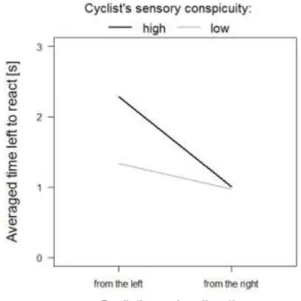
Figure 10: Drivers’ averaged time left to react differed statistically significant dependening on cyclist’s crossing direction (left) and cyclist’s sensory conspicuity (right).

¡Error! No se encuentra el origen de la referencia. (left) shows that drivers had significantly more time left to react to the cyclist coming from the left side (M=1.810s, SE=.176s) compared to the cyclist coming from the right side (M=.993s, SE=.172s). With regard to the main effect of the cyclists sensory conspicuity (see ¡Error! No se encuentra el origen de la referencia., right), drivers had significantly more time left to react on the cyclist with high sensory conspicuity (M=1.648s, SE=.178s) as compared to the cyclist with low sensory conspicuity(M=1.154s, SE=.170s). However, as indicated by the interaction between cyclist’s crossing direction and cyclist’s sensory conspicuity (see Figure 11), the effect of the cyclists crossing direction on driver’s detection performance depends on the state of the cyclists sensory conspicuity. Whereas the average drivers’ detection performance is almost the same for high and low cyclist’s sensory conspicuity when the cyclist is crossing from the right side (low sensory conspicuity: M=.975s, SE=.240s; high sensory conspicuity: M=1.010s, SE=.246s), it is significantly different when the cyclist is

Page | 22 out of 98 crossing from the left side (low sensory conspicuity: M=1.333s, SE=.241s; high sensory conspicuity: M=2.287s, SE=.257s).

Figure 11: Interaction effect between cyclist’s crossing direction and cyclist’s sensory conspicuity.

3.4 CONCLUSIONS

The most relevant car-to-cyclist accident scenario that should be addressed by next-generation VRU systems is a driver approaching a non-signalized intersection or a T-junction and a cyclist crossing from a bicycle lane. Here it was found that the frequency to collide with a cyclist crossing from the right side is higher than with a cyclist crossing from the left side.

The literature review revealed that top-down processes (in terms of erroneous expectations of what potential hazards may occur) may explain both why drivers fail to manage situations with a cyclist from the right more often than with a cyclist from the left (failed-to-look) and why drivers still collide quite frequently with cyclists from the left (looked-but-failed-to-see). However, top-down processes solely cannot explain why the portion of accidents that happened during night time or dawn is higher for cyclist from the left than for cyclists from the right. An explanation could be that, in general, the drivers bottom-up processes may prevent drivers from colliding with a cyclist within the field of view (such as a crossing cyclist crossing from the left), but at night time or dawn the ability of cyclists to capture the drivers bottom-up processes may be reduced - especially if their sensory conspicuity is poor. As a result, the main goal of the study was to examine how and in which situations drivers bottom-up processes may prevent them from colliding with crossing cyclists when turning right at T-junctions.

Therefore, in a driving simulator study, participants had to turn repeatedly (in several rounds) right at two T-junctions. While in the first two rounds (out of three) the

Page | 23 out of 98 participants experienced the turning situations without crossing cyclists, they were confronted with a crossing cyclist in the last round. Within the study three situational factors were varied: (1) the absence or presence of an additional crossing vehicle from the left side, (2) the cyclists crossing direction and (3) the cyclists sensory conspicuity.

The analyses of the objective detection performance showed two significant main effects: First, on average drivers had more time left to react to the cyclist coming from the left side compared to the cyclist from the right side resulting rather from an earlier detection than a lower approaching speed. This result confirms both (a) two baseline rounds are sufficient to build up erroneous expectations and (b) erroneous expectations bias the driver’s attention allocation towards the left side and thus reduce the drivers’ detection performance for a cyclist coming from the right. In general, this result confirms previous findings (Summala, Pasanen, Räsänen, & Sievänen, 1996). Secondly, the drivers had more time left to react on the cyclist with high sensory conspicuity as compared with a cyclist with low sensory conspicuity. Although the interaction effect between the cyclist’s sensory conspicuity and the cyclists crossing direction was only marginally significant, this result indicates that a higher cyclist’s sensory conspicuity does not per se guarantee an earlier detection by drivers. Here it was found that when the cyclist is coming from the right side, then the cyclist’s sensory conspicuity had only little influence on the driver’s detection performance. In contrast, in driving situations with a cyclist coming from the left side drivers detected the cyclist with high sensory conspicuity much earlier than the cyclist with a low sensory conspicuity. As a result, future studies which examine the effectiveness of several measures to increase the cyclist’s sensory conspicuity (e.g., fluorescent or retro-reflective clothing) have to take different driving situations into account.

Moreover, the enhanced detection performance of salient cyclists crossing from the left indicate that the drivers bottom-up processes may prevent the driver from overlooking the cyclist - especially if drivers do not account for cyclists at all. As a result, bottom-up processes can be considered as a natural defense system and are at least as important as top-down processes for traffic safety. However, future assistance systems should contribute to increase the cognitive conspicuity for cyclists as the results have shown that cyclists coming from the left side with low salience have not been detected considerably earlier as cyclists coming from the right side.

The initial hypothesis, that the additional crossing traffic could have an influence on the detection performance of drivers for crossing cyclists, could not be confirmed. One reason for this could be that drivers were expecting crossing traffic at one of the two junctions. Consequently, it could be assumed that drivers expected crossing traffic at each T-junction independently if they really experienced crossing traffic at this particular T-junction in the previous rounds or not.

Page | 24 out of 98

4 E

#2

“

D

’

A

DRIVER MODELS

”

4.1 METHODS

4.1.1 Methodology

The aim of the TME study was to determine the acceptance of drivers to a Forward Collision Warning (FCW) system based on a comfort boundaries model. The comfort boundaries model was obtained from a previous study (DIV project) between TME, Autoliv and Chalmers [Boda et al. (2018)]. One of the aims of the DIV project was to analyse the brake onset of drivers (defined during the study as comfort boundary) when encountering a cyclist crossing the road in an intersection, as presented in Figure 14. Participants were instructed to drive and behave in the same way they would during normal traffic. The study was conducted in a driving simulator and in a test track using the same scenario. Boda et al. (2018) concluded that the moment in time when the cyclist first becomes visible to the driver (time to arrival visibility, 𝑇𝑇𝐴𝑣𝑖𝑠𝑖𝑏𝑖𝑙𝑖𝑡𝑦), had the biggest effect on the brake onset of the driver. The model that describes the brake onset dependant on the visible time of the cyclist. For the present study, the warning inside the comfort boundary was selected as the asymptotic value and the warning outside the comfort boundary was selected as the value below the lower 95% value.

The aim of the study conducted for PROSPECT was to determine the validity of DIV’s comfort model as a model to develop more acceptable warning times. The study was conducted using the AUDI Vehicle In the Loop (VIL) system.

4.1.2 Test setup

The VIL is a virtual reality simulator, which is coupled with a real car, i.e. the participant receives vestibular, kinesthetic and auditory feedback from driving a real car while he/she perceives the simulated environment from the traffic simulation (see Figure 12).

Figure 12: The Vehicle in the loop system used for TME study

The simulated environment was created using the tool-chain VTD (Virtual Test Drive) for driving simulation applications. The road environment included parking lots, houses, stores, signs, sidewalks, cycle paths and oncoming car traffic besides the intersection of interest (see Figure 13).

Page | 25 out of 98 Figure 13. Simulated road environment realized for the TME study

Regarding the design of the warning, a visual-acoustic warning strategy was chosen. When participants approached the intersection of interest, both an acoustic signal and a visual icon within the instrument cluster are displayed once the participant reached a certain distance. To obtain comparable results, all participants were instructed to control the speed by activating the function Adaptive Cruise Control (ACC). The manipulation of the triggered signals was realized by the ADTF software. Simultaneously, the ADTF-software was used to record the driving data (i.e. actual vehicle speed, longitudinal acceleration etc.).

4.1.3 Research design and scenario

For the PROSPECT study, two warnings were tested: one inside the comfort boundaries and one outside the comfort boundaries of the drivers. The timings of the warning were calculated using the above-mentioned comfort boundary model obtained during DIV project. The scenario tested was the same scenario as in the DIV project: a cyclist crossing from the right (Figure 14). For the present study, the cyclist becomes visible at time to collision (TTC) of 4 seconds, i.e. 4 seconds before the car reaches the intersecting point between the vehicle and cycist paths.

Page | 26 out of 98 In order to ensure that the cyclist does not become visible before a TTC of 4s, a blue wall (sight obstruction) on the right leg of the intersection was simulated (see Figure 15). Regarding the resulting warning times, a warning time inside the comfort boundaries of 2.6 s (asymptotic value of the model at TTC=4 seconds) and a warning time outside the comfort boundaries of 1.7 s (below the lower 95 % value of the model at TTC=4 seconds) was calculated. The hypothesis tested in the present study was that warnings outside the drivers comfort boundary would be better accepted as the situation would be critical in the perspective of the driver compared to the situation where the warning is inside their comfort boundary.

Figure 15: Simulated intersection according to the TME study scenario

4.1.4 Procedure

Participants were asked to drive three times around the test track to become familiar with the simulator and the route (Figure 16). After completing the familiarization phase, participants drove 9 times around the route and encountered 9 different conditions in the AUDI junction. Afterward participants had a break. Following the break, the same participants drove one more time around the route and encountered the cyclist crossing in the TME intersection (TME study). After this, the participant finalized the study and had to complete a survey regarding acceptance and willingness to buy the system experienced during the study.

For the TME study, the first objective was to validate that the model represents comfort boundaries of drivers, i.e. determine if the brake onset of the drivers is close to the warning. During the TME study, participants were asked to brake only after the warning was issued. The instruction given to the participant was the following: “During the second intersection, a warning will be signaled. After the warning is signaled, you are allowed to brake at anytime you find convenient (you decide when to brake depending on when you think the situation becomes critical)”. If a bigger gap was found between the warning time and the brake onset during the warning inside the comfort boundary compared to the gap during the outside boundary, it would indicate that drivers will not feel critical a situation when it is inside their comfort boundaries. The next step would be to determine if the activation time of the warning

Page | 27 out of 98 would have an effect in acceptance (using the answers given during the survey completed at the end of the study). The hypothesis was that a warning outside the comfort boundary of the driver will result in better acceptance as it seen as a critical scenario.

A) B)

Figure 16: A) Route followed by each participants B) Intersection used for TME study

4.1.5 Participants

For the current study, 39 participants took part (32 males, 7 females). Participants were randomly allocated into one of the two groups (warning inside the comfort boundary or warning outside the comfort boundary). For the participants in the “warning inside the comfort boundary” group, the mean age was 23.65 years (SD=3.27) and for the “warning outside the comfort boundary” the mean age was 24.84 years (SD=5.93). The median of frequency of driving per week was “3-5 days” and the median of mileage per year was “20,000-30,000 km” for both groups. 7 participants from the “warning outside the comfort boundary” were removed due to problems with the recorded data.

4.2 RESULTS

4.2.1 Brake onset after warning

The first analysis done was to determine the time gap between the warning and the brake onset. This would determine how critical the situation was felt when the warning was issued. The hypothesis is that the warning inside the comfort boundary would not feel critical compared to the warning outside the comfort boundary. The mean gap time for the “inside comfort boundary” group was 1.32 seconds (SD = 0.99) and for the “outside comfort boundary” group was 0.65 seconds (SD = 0.38), as presented in Figure 17. A two sample t-test was done to compare both groups and it was found that there was a significant statistical difference between both groups (t(29)=2.13, p=0.0421). Behr et al. (2010) found that a participant braking reaction to an expected warning was 0.416 seconds (SD = 0.095). This means that the participants who received the warning outside the comfort boundary reacted almost immediately after the warning, i.e. they felt it was already a critical situation.

Page | 28 out of 98 Figure 17: Time gab between warning time and brake onset time for both scenarios:

inside and outside of the comfort boundaries

4.2.2 Acceptance questionnaire

Participants were asked to complete a survey at the end of the experiment. The survey consisted of 5 questions with a 5-point Likert-scale. The questions were the following:

Do you think the warning was in time? How helpful was the warning to you? How disturbing was the warning to you? Do you think the warning was unnecessary?

If it were available in the market, would you buy it?

A Wilcoxon rank sum test was done to compare the answers given by the participants in both groups. For the first (Was the warning on time?) and third question (Was the warning disturbing?), there was a statistical significant difference between groups. For the first question participants from the “inside comfort boundary” group score a median of 3 (“Just right”) compared to the “outside comfort boundary” group with a median of 5 (“Too late”). This indicates that participants felt that the “outside comfort boundary” warning was issued later than when they would have braked. For the third question, although both groups did not find it disturbing, the “inside comfort boundary” group found the warning more disturbing than the “outside comfort boundary” group.

The second, fourth and fifth question did not show any significant difference between groups. For the second question (Was the warning helpful?) both groups found the warning helpful (both groups score a median of 4 which meant “Somewhat helpful”). For the fourth question, both groups found the warning necessary. And for the fifth question, both groups tended towards agreeing to buy the system, regardless of the

Page | 29 out of 98 timing of the alarm. Table 3 shows the results of the analysis of the survey responses and Figure 18 shows the results of the survey by group.

Table 3: Responses per group to the five questions in the survey given to the participants after the drive

Question Median “inside comfort

boundary” Median “outside comfort boundary” p-value Warning on time?

3 (“Just right”) 5 (“Too late”) 0.0013 *

Warning was helpful?

4 (“Somewhat helpful”) 4 (“Somewhat helpful”) 0.5206 Warning was

disturbing?

2.5 (between “Not

disturbing” and “Neither/Nor”

2 (“Not disturbing”) 0.0308 * Warning was

unnecessary?

2 (“Not unnecessary”) 3 (“Neither/Nor”) 0.6622

Willingness to buy?

3.5 (between “Neither/Nor” and “Agree”)

4 (“Agree”) 0.1674

Page | 31 out of 98 Figure 18: Survey results for both groups

4.2.3 Correlation

A spearman rank correlation test was performed to determine the effect of the gap between the warning and the braking time and the willingness to buy a PROSPECT-like system. It was found a slightly significant negative correlation between the time gap and willingness to buy (r(31)= -0.3478, p=0.0552). This means that the closer the warning time is to the time when a driver would normally brake, i.e. when the driver feels a situation is critical, the more the driver will be willing to buy a PROSPECT-like system. It is therefore necessary to understand the comfort boundaries of people to avoid signaling warnings too early and reduce the acceptance of people towards the system.

4.3 CONCLUSIONS

The study demonstrated that it is possible to use comfort boundary models to determine more acceptable warning times for drivers. The braking reaction towards the warning outside the comfort boundary confirmed that the warning was issued when the scenario was already critical for the driver (outside the driver’s comfort boundary). In similar way, the long gap between the braking onset and the warning inside the comfort boundary confirms that the driver was still in a “comfort zone” during the warning. This validates the comfort boundaries of the model. Secondly, through the surveys’ answers, it was found that the warning outside the comfort boundary was less disturbing than the one inside the comfort boundary. It was also found that people would be more willing to buy the warning system that has the warning outside the comfort boundary. Although this was tested only in one scenario,

Page | 32 out of 98 it is an important step to validate driver models as a method to develop better accepted warnings by the drivers.

Page | 33 out of 98

5 E

#3

“U

N

A

”

5.1 OVERVIEW

The University of Nottingham (UoN) conducted a large-scale, longitudinal driving simulator study (N=48) to evaluate system functionality (T7.2) and issues of driver trust and acceptance (T7.3). Adopting the methodology developed by Large et al. (2017), the study took place in the Human Factors driving simulator at the University of Nottingham. The driving simulator is a medium-fidelity, fixed-based simulator comprising an Audi TT car located within a curved screen, affording ∼270° forward and side image of the driving scene via three overhead HD projectors. A thrustmaster force-feedback steering wheel and pedal set are faithfully integrated with the original Audi steering wheel and pedals. STISIM Drive (version 3) was used to create an urban driving environment.

5.1.1 Methodology

Forty-eight experienced drivers were invited to attend at the same time on each of five consecutive days (Monday to Friday), and completed the same journey, which was presented to them as their daily commute.

The journey began on the outskirts of an urban environment and continued through the city. Towards the end of the drive, which lasted approximately 10-15 minutes, participants were asked to make a left turn. Shortly after this, drivers were advised that they had reached their destination and were asked to safely stop the vehicle. The simulator was modified to replicate the PROSPECT functionality (utilising an audible warning and emergency braking intervention, as specified by D5.2). However, this was only triggered once during the week, when a cyclist was detected crossing the final road into which driver was turning. The intention was to replicate the ‘likely’ frequency of activation associated with a ‘real’ system. During the remainder of the study (i.e. all other visits to the simulator), the driving experience was routine, i.e. no cyclist hazard present during the manoeuvre. This approach improves upon other ‘single-visit’ simulator studies in that participants are not inundated with warnings and interventions in rapid succession (which can provide a false representation of the system, and is therefore likely to generate a poor assessment of acceptance), but rather experience the system only occasionally. The study explored PROSPECT use-case 2 (see Figure 19), whereby a vehicle and a cyclist are approaching a crossing from the same direction. The cyclist wants to continue straight ahead while the vehicle intends to turn to the right. A collision risk occurs when the cyclist starts crossing the road at the instant when the car starts turning to the right.

Half of the participants (n=24) experienced a ‘true-positive’ system intervention, i.e. the system identified a critical incident – in this case, the cyclist crosses the road into which they were turning, and a warning is provided, followed by emergency braking (Figure 20).

Page | 34 out of 98 The remainder of the participants (n=24) experienced a ‘false-positive’ intervention, i.e. a cyclist is detected as they approach the roadside and a warning is provided, followed by emergency braking. However, in this case, the cyclist actually stops before entering the roadway (Figure 21).

As such, it was expected that the latter intervention would be perceived as a ‘false-alarm’ as the cyclist did not actually enter the roadway. Nevertheless, the situation is still arguably ‘critical’ in so far as the system predicted that a collision would take place based on the current trajectories of both parties, and also likely to be highlighted by the PROSPECT sytem. Consequently, understanding the effect on driver acceptance and acceptability is still highly relevant.

During the study, acceptance was subsequently assessed utilising the approach developed as part of PROSPECT and documented within D7.2. In this case, only the ‘during’ and ‘after’ questionnaires (in addition to capturing demographic data) were employed to avoid biasing the results (i.e., to avoid creating expectations of behaviour from ‘the PROSPECT system). It was also felt that this more accurately reflected a ‘real-world’ situation, whereby drivers would not necessarily be aware of the operational intricacies of active safety systems in their vehilce, and therefore an emergency intervention by the car would likely be unexpected.

Figure 19- PROSPECT Use-Case 2 replicating in the study (Note: testing took place in the UK, and therefore the scenario was mirrored)