Dynamic estimation for medical data management in a cloud federation

HAL Id: hal-02285762

https://hal.archives-ouvertes.fr/hal-02285762

Submitted on 13 Sep 2019

HAL is a multi-disciplinary open access

archive for the deposit and dissemination of

sci-entific research documents, whether they are

pub-lished or not. The documents may come from

teaching and research institutions in France or

abroad, or from public or private research centers.

L’archive ouverte pluridisciplinaire HAL, est

destinée au dépôt et à la diffusion de documents

scientifiques de niveau recherche, publiés ou non,

émanant des établissements d’enseignement et de

recherche français ou étrangers, des laboratoires

publics ou privés.

Dynamic estimation for medical data management in a

cloud federation

Trung-Dung Le, Verena Kantere, Laurent Orazio

To cite this version:

Trung-Dung Le, Verena Kantere, Laurent Orazio. Dynamic estimation for medical data management

in a cloud federation. International Workshop on Data Analytics solutions for Real-LIfe APplications,

Mar 2019, Lisbon, Portugal. �hal-02285762�

Dynamic estimation for medical data management in a

cloud federation

Trung-Dung Le

Univ Rennes CNRS, IRISA Lannion, France trung-dung.le@irisa.fr

Verena Kantere

University of Ottawa School of Electrical Engineering and

Computer Science Ottawa, Canada vkantere@uOttawa.ca

Laurent d

′

Orazio

Univ Rennes CNRS, IRISA Lannion, France laurent.dorazio@irisa.fr

ABSTRACT

Data sharing is important in the medical domain. Sharing data al-lows large-scale analysis with many data sources to provide more accurate results (especially in the case of rare diseases with small local datasets). Cloud federations consist in a major progress in sharing medical data stored within different cloud platforms, such as Amazon, Microsoft, Google Cloud, etc. It also enables to ac-cess distributed data of mobile patients. The pay-as-you-go model in cloud federations raises an important issue in terms of Multi-Objective Query Processing (MOQP) to find a Query Execution Plan according to users preferences, such as response time, money, quality, etc. However, optimizing a query in a cloud federation is complex with increasing heterogeneity and additional variance, especially due to a wide range of communications and pricing models. Indeed, in such a context, it is difficult to provide accurate estimation to make relevant decision. To address this problem, we present Dynamic Regression Algorithm (DREAM), which can provide accurate estimation in a cloud federation with limited historical data. DREAM focuses on reducing the size of historical data while maintaining the estimation accuracy. The proposed al-gorithm is integrated in Intelligent Resource Scheduler, a solution for heterogeneous databases, to solve MOQP in cloud federations and validate with preliminary experiments on a decision support benchmark (TPC-H benchmark).

1

INTRODUCTION

Medical data sharing is full of promises. It allows large-scale med-ical data analysis to diagnose diseases more accurately. To reach this goal, the distributed clinics need to optimize queries on shared medical data with data sources in a cloud federation. For instance, in health-care, information of a given patient may be owned by different hospitals that may use various providers. Pay-as-you-go models in cloud federations and elasticity thus raise an important issue in terms of Multi-Objective Query Processing (MOQP) to find a Query Execution Plan (QEP) according to users preferences, such as time, money, quality, etc. However, optimizing queries in a cloud federation raises issues of heterogeneity and variability of cloud environment, such as wide-range communications and pricing models.

In variable environment like a cloud federation with various database systems, we should build a model to estimate the cost values for the MOQP. A cloud federation may rely on various hardware and systems. In addition, it also depends on the variety of physical machines, load evolution and wide-range communica-tions. As a consequence, estimation is complex with the variability

© 2019 Copyright held by the author(s). Published in the Workshop Proceedings of the EDBT/ICDT 2019 Joint Conference (March 26, 2019, Lisbon, Portugal) on CEUR-WS.org

of environment. In this context, a challenging problem is how to estimate accurate values for MOQP without precise knowledge of execution environment in a cloud federation consisting of different sites.

Cost modeling can be classified into two classes: without [23, 26, 34] and with machine learning algorithms [11]. How-ever, in a cloud federation with variability and different systems, cost functions may be quite complex. In the first class, cost mod-els introduced to build optimal group of queries [23] are limited to MapReduce [8]. Besides, PostgreSQL cost model [34] aims to predict query execution time for this specific relational Data Base Management system. Moreover, OptEx [26] provides esti-mated job completion times for Spark [28] with respect to the size of the input dataset, the number of iterations, the number of nodes composing the underlying cloud. However, these papers only mention the estimation of execution time for a job, not for other metrics, such as monetary cost. Meanwhile, various machine learning techniques are applied to estimate execution time in re-cent researches [1, 15, 30, 35]. They predict the execution time by many machine learning algorithms. They treated the database system as a black box and try to learn a query running time pre-diction model using the total information for training and testing in the model building process. It may lead to the use of expired information. In addition, most of these solutions solve the opti-mization problem with a scalar cost value and do not consider multi-objective problems.

In this paper, we introduce a medical system on a cloud feder-ation called Medical Data Management System (MIDAS). It is based on the Intelligent Resource Scheduler (IReS) [11], an open source platform for complex analytics workflows executed over multi-engine environments. In particular, we focus on Dynamic Regression Algorithm (DREAM) to provide accurate estimation with low computational cost. DREAM is then implemented and validated with preliminary experiments on a decision support benchmark (TPC-H benchmark [31]).

The remaining of this paper is organized as follows. Section 2 presents the research background. DREAM is presented in Sec-tion 3, while SecSec-tion 4 presents experiments to validate DREAM. Finally, Section 5 concludes this paper and lists some perspectives.

2

BACKGROUND

Our work is a part of the MIDAS project, which aims to provide a data management system for cloud federation. In this section, we introduce an architecture of the system, concepts and techniques, allowing us to implement the proposed medical data management on a cloud federation.

First of all, an overview of MIDAS and the benefits of cloud federation where our system is built on are introduced. After that, an open source platform, which helps our system managing and executing workflows over multi-engine environments is described.

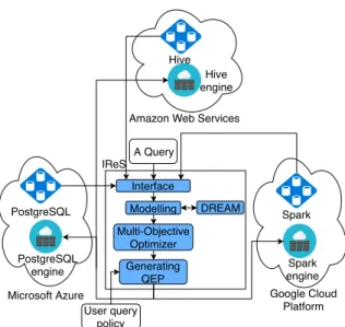
Interface User query policy Modelling Generating QEP Hive engine Multi-Objective Optimizer Hive  A Query PostgreSQL engine PostgreSQL Spark engine Spark Amazon Web Services

Microsoft Azure Google Cloud Platform IReS

DREAM

Figure 1: Architecture of MIDAS.

The concept of Pareto plan set related to MOQP in MIDAS is then defined. In addition, Multiple Linear Regression is also introduced as the basic foundation of our proposed algorithm for MOQP.

2.1

MIDAS

MIDAS is a medical data management system for cloud federa-tion. The proposal aims to provide query processing strategies to integrate existing information systems (with their associated cloud provider and data management system) for clinics and hospitals. Figure 1 presents an overview of the system. Integrating the sys-tem within a cloud federation allows to choose the best strategy for MOQP. The different cloud resource pools allow the system to run in the most appropriate infrastructure environments. The system can optimize workflows between different data sources on different clouds, such as Amazon Web Services [3], Microsoft Azure [4] and Google Cloud Platform [16]. The proposed system is developed based on the Intelligent Resource Scheduler (IReS) for complex analytics workflows executed over multi-engine envi-ronments on a cloud federation.

2.2

Cloud federation

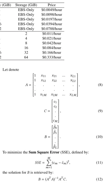
A cloud federation enables to interconnect different cloud com-puting environments. Cloud comcom-puting [2] allows to access on demand and configurable resources, which can be quickly made available with minimal maintenance. According to the pay-as-you-go pricing model, customers only pay for resources (storage and computing) that they use. Cloud Service Providers (CSP) supply a pool of resources, development platforms and services. There are many CSPs on the market, such as Amazon, Google and Microsoft, etc., with different services and pricing models. For example, Table 1 shows the pricing of instances in two cloud providers. The price of Amazon instances are lower than the price of Microsoft instances, but the price of Amazon is without storage. Hence, depending on the demand of a query, the monetary cost is lower or higher at a specific provider.

In medical domain, cloud federation may lead to query data on different clouds. For example, mobile patient data can be analyzed with many distributed sources of data to provide more accurate results. Data management in a cloud federation is thus a critical

issue in terms of multi-engine environment and Multi-Objective Query Processing.

2.3

Pareto plan set

Let a queryq be an information request from databases, presented by a set Q of tables. A Query Execution Plan (QEP) includes an ordered set of operators (select, project, join, etc.). The set of QEPsp of q is denoted by symbol P. The set of operators is denoted by O. A planp can be divided into two sub-plans p1and

p2ifp is the result of function Combine(p1, p2, o), where o ∈ O.

The execution cost of a QEP depends on parameters, which values are not known at the optimization time. A vectorx denotes parameters value and the parameter space X is the set of all possible parameter vectorsx. In MOQP,N is denoted as the set of n cost metrics. We can compare QEPs according to n cost metrics which are processed with respect to the parameter vectorx and cost functionscn(p, x). Let denote C as the set of cost function c. Letp1, p2∈ P,p1dominatesp2if the cost values according to

each cost metric of planp1is less than or equal to the

correspond-ing values of planp2in all the space of parameter X. That is to

say:

C(p1, X) ⪯ C(p2, X) | ∀n ∈ N, ∀x ∈ X : cn(p1, x) ≤ cn(p2, x).

(1) The functionDom(p1, p2) ⊆ X yields the parameter space region

wherep1dominatesp2[32]:

Dom(p1, p2)= {x ∈ X | ∀n ∈ N : cn(p1, x) ≤ cn(p2, x)}. (2)

Assume that in the areax ∈ A, A ⊆ X,p1dominatesp2,C(p1, A) ⪯

C(p2, A), Dom(p1, p2)= A ⊆ X. p1strictly dominatesp2if all

values for the cost functions ofp1are less than the corresponding

values forp2[32], i.e.

StriDom(p1, p2)= {x ∈ X | ∀n ∈ N : cn(p1, x) < cn(p2, x)}.

(3) A Pareto region of a plan is a space of parameters where there is no alternative plan has lower cost than it [32]:

PaReд(p) = X \ ( Ø

p∗_{∈ P}

StriDom(p∗_{, p)).}

(4)

2.4

IReS

Intelligent Multi-Engine Resource Scheduler (IReS) [11] is an open source platform for managing, executing and monitoring complex analytics workflows. IReS provides a method of opti-mizing cost-based workflows and customizable resource manage-ment of diverse execution and various storage engines. Interface is the first module which is designed to receive information on data and operators, as shown in Figure 1. The second module is Modelling, as shown in Figure 1, is used to predict the exe-cution time by a model chosen by comparing machine learning algorithms. For example, Least squared regression [25], Bagging predictors [6], Multilayer Perceptron in WEKA framework [33] are used to build the cost model in Modelling module. The mod-ule tests many algorithms and the best model with the smallest error is selected. It guarantees the predicted values as the best one for estimating process. Next module, Multi-Objective Opti-mizer, optimizes MOQP and generates a Pareto QEP set. In Multi-Objective problem, the objectives are the cost functions user con-cerned, such as the execution time, monetary, intermediate data, etc. Multi-Objective Optimization algorithms can be applied to the Multi-Objective Optimizer. For instance, the algorithms based on Pareto dominance techniques [7, 9, 10, 19, 21, 22, 29, 36, 37]

Table 1: Example of instances pricing.

Provider Machine vCPU Memory (GiB) Storage (GiB) Price

Amazon a1.medium 1 2 EBS-Only $0.0049/hour

a1.large 2 4 EBS-Only $0.0098/hour

a1.xlarge 4 8 EBS-Only $0.0197/hour

a1.2xlarge 8 16 EBS-Only $0.0394/hour

a1.4xlarge 16 32 EBS-Only $0.0788/hour

Microsoft B1S 1 1 2 $0.011/hour B1MS 1 2 4 $0.021/hour B2S 2 4 8 $0.042/hour B2MS 2 8 16 $0.084/hour B4MS 4 16 32 $0.166/hour B8MS 8 32 64 $0.333/hour

are solutions for Multi-objective Optimization problems. Finally, the system selects the best QEP based on user query policy and Pareto set. The final query plan is run on multiple engines, as shown in Figure 1.

2.5

Multiple Linear Regression

A cost function of Multiple Linear Regression (MLR) model [27] is following defined:

c = β0+ β1x1+ ... + βLxL+ ϵ, (5)

whereβl,l = 0, ..., L, are unknown coefficients, xl, l = 1, ..., L, are

the independent variables, e.g., size of data, computer configura-tion, etc.,c is cost function values and ϵ is random error following normal distribution N (0,σ2) with zero mean and varianceσ2. The fitted equation is defined by:

ˆ

c = ˆβ0+ ˆβ1x1+ ... + ˆβLxL. (6)

EXAMPLE2.1. A query Q could be expressed as follows:

SELECT p.PatientSex, i.GeneralNames

FROM Patient p, GeneralInfo i

WHERE p.UID = i.UID

where Patient table is stored in cloud A and uses Hive database en-gine [18], while GeneralInfo table is in cloud B with PostgreSQL database engine [24]. This scenario leads to concern two metrics of monetary cost and execution time cost. We can use the cost functions which depend on the size of tables of Patient and Gener-alInfo. Besides, the configuration and pricing of virtual machines cloud A and B are different. Hence, the cost functions depend on the size of tables and the number of virtual machines in cloud A and B. ˆ ct i _{= ˆβ} t0+ ˆβt1xP a+ ˆβt2xGe+ ˆβt3xnodeA+ ˆβt4xnode B ˆ cmo_{= ˆβ} m0+ ˆβm1xP a+ ˆβm2xGe+ ˆβm3xnodeA+ ˆβm4xnode B

wherecˆt i, ˆcmo are execution time and monetary cost function; xP a, xGeare the size of Patient and GeneralInfo tables,

respec-tively, andx_nodeA, x_{node B} are the number of virtual machines created to run queryQ.

There areM historical data, each of them associates with a re-sponsecm, which can be predicted by a fitted valuecˆmcalculated

from correspondingx_lmas follows: ˆ cm= ˆβ0+ ˆβ1x1m+ ... + ˆβLxLm;m = 1, ..., M. (7) Let denote A =           1 x11 x21 ... xL1 1 x12 x22 ... xL2 . . . . . . . . . . 1 x1M x2M ... xLM           , (8) C =           c1 c2 . . cM           , (9) B =           ˆ β0 ˆ β1 . . ˆ βL           . (10)

To minimize the Sum Square Error (SSE), defined by: SSE =

M

Õ

m=1

(cm−cˆm)2, (11)

the solution forB is retrieved by:

B = (AT_A)−1_AT_{C. (12)}

2.6

Motivation

Our proposed method is integrated into Modelling module to pre-dict the cost values with low computational cost in MOQP of a cloud environment. However, the machine learning algorithms in Modelling module of IReS need entire of training datasets. It may lead to use expired information. Hence, the proposal algo-rithm aims to improve the accuracy of estimated values with low computational cost.

In addition, MOQP could be solved by Multi-objective Opti-mization algorithms or the Weighted Sum Model (WSM) [17]. However, Multi-objective Optimization algorithms may be se-lected thanks to their advantages when comparing with WSM. The optimal solution of WSM could be not acceptable, because of an inappropriate setting of the coefficients [13]. Furthermore, the research in [20] proves that a small change in weights may result in significant changes in the objective vectors and signif-icantly different weights may produce nearly similar objective vectors. Moreover, if WSM changes, a new optimization process will be required. Hence, our system applies a Multi-objective Op-timization algorithm to the Multi-Objective Optimizer to find a Pareto-optimal solution.

In conclusion, our solution aims to improve the accuracy of cost value prediction with low computational cost and to solve MOQP by Multi-objective Optimization algorithm in a cloud federation environment. To provide accurate estimation while reducing the number of previous measures, our algorithm is proposed based on Multiple Linear Regression.

3

DYNAMIC REGRESSION ALGORITHM

Most of cost models [12, 23, 34] depend on the size of data. Hence, our cost functions are functions of the size of data. In particular, cost function and fitted value of Multiple Linear Re-gression model are previously defined in Section 2.5. The bigger M for sets {cm, xlm} is, the more accurate MLR model usually is.

However, the computers is slowing down whenM is too big. Furthermore, the target of Multi-Objective Query Processing is the Multi-Objective Optimization Problem [36], which is defined by:

minimize(F (x) = (f1(x), f2(x)..., fK(x))T), (13)

wherex = (x1, ..., xL)T ∈Ω ⊆ RLis an L-dimensional vector of

decision variables,Ω is the decision (variable) space and F is the objective vector function, which containsK real value functions. In general, there is no point inΩ that minimizes all the objec-tives together. Pareto optimality is defined by trade-offs among the objectives. If there is no pointx ∈ Ω such that F (x) dominates F (x∗_),x∗ _{∈Ω, x}∗

is called Pareto optimal andF (x∗) is called a Pareto optimal vector. Set of all Pareto optimal points is the Pareto set. A Pareto front is a set of all Pareto optimal objective vectors. Generating the Pareto-optimal front can be computationally ex-pensive [5]. In cloud environment, the number of equivalent query execution plans is multiplied.

EXAMPLE3.1. Assuming that a query is processed on Amazon EC2. If the pool of resources includes 70 vCPU and 260GB of memory, the number of different configurations to execute this query is thus 70 x 260 = 18,200. Hence, the system can generate 18,200 equivalent QEPs from a give execution plan.

Example 3.1 shows that a query execution plan can generate multiple equivalent QEPs in cloud environment. The smallerM for sets {cm, xlm} is, the faster speed for the estimation cost process

of Multi-Objective Query Processing for a QEP is. In the system of computationally expensiveness in cloud environment as in Example 3.1, a small reduction of computation for an equivalent QEP estimation will become significant for a large number of equivalent QEPs estimation.

The most important idea is to estimate MLR quality by using the coefficient of determination. The coefficient of determination [27] is defined by:

R2_{= 1 − SSE/SST, (14)}

whereSSE is the sum of squared errors and SST represents the amount of total variation corresponding to the predictor variableX . Hence,R2shows the proportion of variation in cost given by the Multiple Linear Regression model of variableX . For example, the model givesR2= 0.75 of time response cost, it can be concluded that 3/4 of the variation in time response values can be explained by the linear relationship between the input variables and time response cost. Table 2 presents an example of MLR with different number of measures. The smallest dataset isM = L + 2 = 4 [27], whereM is the size of previous data and L is the number of variables in Equation (5). In general,R2increases in parallel withM. In particular, R2should be greater than 0.8 to provide a sufficient quality of service level. As a consequence,M should

Table 2: Using MLR in different size of dataset.

Cost x1 x2 M R2 20.640 0.4916 0.2977 15.557 0.6313 0.0482 20.971 0.9481 0.8232 24.878 0.4855 2.7056 4 0.7571 23.274 0.0125 2.7268 5 0.7705 30.216 0.9029 2.6456 6 0.8371 29.978 0.7233 3.0640 7 0.8788 31.702 0.8749 4.2847 8 0.8876 20.860 0.3354 2.1082 9 0.8751 32.836 0.8521 4.8217 10 0.8945

be greater than 5 to provide enough accuracy. Hence, when the system requires the minimum values ofR2is equal to 0.8,M > 6 is not recommended. In general,R2still rises up whenM goes up. Therefore, we need to determine the model which is sufficient suitable by the coefficient of determination.

Training set DREAM

coefficient of determination

New training

set Modelling

Figure 2: DREAM module.

Our motivation is to provide accurate estimation while reducing the number of previous measures based onR2. We thus propose DREAM as a solution for cloud federation and their inherent variance, as shown in Table 2. DREAM uses the training set to test the size of new training dataset. It depends on the predefined coefficient of determination. The new training set is generated in oder to have the updated value and avoid using the expired information. With the new training set, Modelling uses less data in building model process than the original approach.

Cost modeling without machine learning [23, 26, 34] often uses the size of data to estimate the execution time for the specific system. Besides, the machine learning approach [11, 33] can use any information to estimate the cost value. Hence, our algorithm uses the size of data as variables of DREAM. In (6),c is the costˆ value, which needs to be estimated in MOQP, andx1, x2, . . . are

the information of system, such as size of input data, the number of nodes, the type of virtual machines. IfR2≥R2_{r equir e}, where R2

r equir esis predefined by users, the model is reliable. In contrast,

it is necessary to increase the number of set value. Algorithm 1 shows a scheme as an example of increasing value set:m = m + 1. In this paper, we focus on the accuracy of execution time es-timation with the low computational cost in MOQP. The origi-nal optimization approach in IReS uses Weighted Sum Model [17] with user policy to find the best candidate. However, Multi-objective Optimization algorithms have more advantages than WSM [13, 20]. Hence, after having a set of predicted cost func-tion values for each query plan, a Multi-objective Optimizafunc-tion algorithm, such as Non-dominated Sorting Genetic Algorithm II [10] is applied to determine a Pareto plan set. At the final step, the weight sum model S and the constraint B associated with the

Algorithm 1 Calculate the predict value of multi-cost function

1: function ESTIMATECOSTVALUE(R_{r equir e}2 , X, Mmax) 2: forn = 1 to N do

3: R2n← ∅ //with all cost function

4: end for

5: m = L + 2 //at least m = L + 2

6: while (anyR_n2 < R2_{n−r equir e}) andm < Mmaxdo 7: forcˆn(p) ⊆ ˆcN(p) do 8: R2_n= 1 − SSE/SST 9: cˆn= ˆβn0+ ˆβn1x1+ ... + ˆβnLxL 10: end for 11: m = m + 1 12: end while 13: returnˆcN(p) 14: end function Initial Population Objective values Fitness Distribution Genetic Operation Insert Parent Satisfied Termination Criteria? Termination Population All Candidates Weighted Sum Model Values Comparing Scalar Values Weighted Sum Model Values Comparing Scalar Value

The best QEP

The best QEP

Multi-Objecitve Optimization based on Genetic Algorithm

Multi-Objecitve Optimization based on Weighted Sum Model

Figure 3: Comparing two MOQP approaches

Algorithm 2 Select the best query plan in P

1: function BESTINPARETO(P, S, B)

2: P_B←p ∈ P|∀n ≤ |B| : cn(p) ≤ Bn 3: ifPB, ∅ then

4: returnp ∈ PB|C(p) = min(W eiдhtSum(PB, S)) 5: else

6: returnp ∈ P|C(p) = min(W eiдhtSum(P, S))

7: end if

8: end function

user policy are used to return the best QEP for the given query [17]. In particular, the most meaningful plan will be selected by comparing function values with weight parameters betweencˆn

[17] at the final step, as shown in Algorithm 2. Figure 3 shows the different between two MOQP approaches.

Our algorithms are developed based on the MLR described above usingxifor size of data andci for the metric cost, such as

the execution time, energy consumption, etc.

Table 3: Comparison of mean relative error with 100MiB TPC-H dataset. Query BMLN BML2N BML3N BML DREAM 12 0.265 0.459 0.220 0.485 0.146 13 0.434 0.517 0.381 0.358 0.258 14 0.373 0.340 0.335 0.358 0.319 17 0.404 0.396 0.267 0.965 0.119

4

EVALUATION

DREAM has been implemented on top of IReS platform. It has been validated with experiments.

4.1

Implementation

Our experiments are executed on a private cloud [14] with a cluster of three machines. Each node has four 2.4 GHz CPU, 80 GiB Disk, 8 GiB memory and runs 64-bit platform Linux Ubuntu 16.04.2 LTS. The system uses Hadoop 2.7.3 [24], Hive 2.1.1 [18], PostgreSQL 9.5.14 [24], Spark 2.2.0 [28] and Java OpenJDK Runtime Environment 1.8.0. IReS platform is used to manage data in multiple database engine and deploy the algorithms.

4.2

Experiments

TPC-H benchmark [31] with two datasets of 100MB and 1GB is used to have experiments with DREAM. Experiments with TPC-H benchmark are executed in a multi-engine environment consisting of Hive[18] and PostgreSQL[24] deployed on a private cloud [14]. In TPC-H benchmark, the queries related to two tables are 12, 13, 14 and 17. These queries with two tables in two different databases, such as Hive and PostgreSQL, are studied.

4.3

Results

To estimate the quality of DREAM in comparison with other algorithms, Mean Relative Error (MRE), a metric used in [1] is used and described as below:

1 M i=1 Õ M |cˆi−ci| ci , (15)

where M is the number of testing queries,cˆi andci are the predict

and actual execution time of testing queries, respectively. IReS platform uses multiple machine learning algorithms in their model, such as Least squared regression, Bagging predictors, Multilayer Perceptron.

In IReS model building process, IReS tests many algorithms and the best model with the smallest error is selected. It guar-antees the predicted values as the best one for estimating pro-cess. DREAM is compared to the Best Machine Learning model (BML) in IReS platform with many observation window (N , 2N , 3N and no limit of history data). The smallest size of a window, N = L+2 [27], where L is the number of variables, is the minimum data set DREAM requires. As shown in Tables 3 and 4, MRE of DREAM are the smallest values between various observation windows. In our experiments, the size of historical data, which DREAM uses, are very small, aroundN .

5

CONCLUSION

This paper is about medical data management in cloud federa-tion. It introduces Dynamic Regression Algorithm (DREAM) as a part of MIDAS and on top of IReS, an open source platform for

Table 4: Comparison of mean relative error with 1GiB TPC-H dataset. Query BMLN BML2N BML3N BML DREAM 12 0.349 0.854 0.341 0.480 0.335 13 0.396 0.843 0.457 0.487 0.349 14 0.468 0.664 0.539 0.790 0.318 17 0.620 0.611 0.681 0.970 0.536

complex analytics work-flows executed over multi-engine envi-ronments. DREAM aims to address variance in a cloud federation and to provide accurate estimation for MOQP. Preliminary results with DREAM and TPC-H benchmark are quite promising with respect to existing solutions.

In the future, we plan to validate our proposal with more cloud providers (and their associated pricing model and services) and data management systems. We will also define new strategies to choose QEPs in a Pareto Set.

ACKNOWLEDGMENT

The authors would like to thank members of SHAMAN team at Univ Rennes, CNRS, IRISA and University of Ottawa School of Electrical Engineering and Computer Science for insightful comments.

REFERENCES

[1] M. Akdere, U. Çetintemel, M. Riondato, E. Upfal, and S. B. Zdonik. 2012. Learning-based query performance modeling and prediction. International Conference on Data Engineering(2012), 390–401.

[2] Michael Armbrust, Armando Fox, Rean Griffith, Anthony D. Joseph, Randy Katz, Andy Konwinski, Gunho Lee, David Patterson, Ariel Rabkin, Ion Stoica, and Matei Zaharia. 2010. A View of Cloud Computing. Commun. ACM 53, 4 (April 2010), 50–58.

[3] AWS 2018. Amazon Web Services Website. (2018). https://aws.amazon.com/ [4] Azure 2018. Microsoft Azure Website. (2018). https://azure.microsoft.com/ [5] Lucas S. Batista. 2012. Performance Assessment of Multiobjective

Evolution-ary Algorithms. 7 (2012).

[6] Leo Breiman. 1996. Bagging predictors. Machine Learning 24 (1996), 123– 140.

[7] Carlos A. Coello Coello, David A. Van Veldhuizen, and Gary B. Lamont. 2002. Evolutionary Algorithms for Solving Multi-Objective Problems (Genetic and Evolutionary Computation).

[8] Jeffrey Dean and Sanjay Ghemawat. 2008. MapReduce: Simplified Data Processing on Large Clusters. Commun. ACM 51 (Jan. 2008), 107–113. [9] Kalyanmoy Deb and Himanshu Jain. 2013. An Evolutionary Many-Objective

Optimization Algorithm Using Reference-point Based Non-dominated Sorting Approach, Part I: Solving Problems with Box Constraints. IEEEXplore 18 (2013).

[10] Kalyanmoy Deb, Amrit Pratap, Sameer Agarwal, and T. Meyarivan. 2002. A fast and elitist multiobjective genetic algorithm: NSGA-II. IEEE Trans. Evol. Comput.6 (2002), 182–197.

[11] K. Doka, Ni Papailiou, D. Tsoumakos, C. Mantas, and N. Koziris. 2015. IReS: Intelligent, Multi-Engine Resource Scheduler for Big Data Analytics Work-flows. In SIGMOD ’15.

[12] H. M. Fard, R. Prodan, J. J. D. Barrionuevo, and T. Fahringer. 2012. A Multi-objective Approach for Workflow Scheduling in Heterogeneous Environments. 12th IEEE/ACM(2012).

[13] C. M. Fonseca and P. J. Fleming. 1995. An Overview of Evolutionary Algo-rithms in Multiobjective Optimization. Evolutionary Computation 3, 1 (Mar. 1995), 1–16.

[14] Galactica 2018. The Galactica Website. (2018). https://horizon.isima.fr [15] A. Ganapathi, H. Kuno, U. Dayal, J. L. Wiener, A. Fox, M. Jordan, and D.

Patterson. 2009. Predicting Multiple Metrics for Queries: Better Decisions Enabled by Machine Learning. In 2009 IEEE 25th International Conference on Data Engineering. 592–603.

[16] Google 2018. Google Cloud Website. (2018). https://cloud.google.com/ [17] Florian Helff and Laurent Orazio. 2016. Weighted Sum Model for

Multi-Objective Query Optimization for Mobile-Cloud Database Environments. In EDBT/ICDT Workshops.

[18] Hive 2018. The Hive Website. (2018). http://hive.apache.org/

[19] Himanshu Jain and Kalyanmoy Deb. 2014. An evolutionary many-objective optimization algorithm using reference-point based nondominated sorting ap-proach, Part II: Handling constraints and extending to an adaptive approach.

IEEE Transactions on Evolutionary Computation18 (2014), 602–622. [20] Salman A. Khan and Shafiqur Rehman. 2013. Iterative non-deterministic

algorithms in on-shore wind farm design: A brief survey. Renewable and Sustainable Energy Reviews19 (2013), 370 – 384.

[21] J. Knowles and D. Corne. 1999. The Pareto archived evolution strategy: a new baseline algorithm for Pareto multiobjective optimisation. In 1999 Congress on Evolutionary Computation-CEC99 (Cat. No. 99TH8406), Vol. 1. 98–105. [22] Trung-Dung Le, Verena Kantere, and Laurent d’Orazio. 2018. An efficient

multi-objective genetic algorithm for cloud computing: NSGA-G. In Interna-tional Workshop on Benchmarking, Performance Tuning and Optimization for Big Data Applications (BPOD@BigData). Seattle, WA, USA.

[23] T. Nykiel, M. Potamias, C. Mishra, G. Kollios, and N. Koudas. 2010. MRShare: sharing across multiple queries in MapReduce. VLDB Endowment (2010). [24] PostgreSQL 2018. The PostgreSQL Website. (2018). https://www.postgresql.

org/

[25] Peter J. Rousseeuw and Annick M. Leroy. 1987. Robust regression and outlier detection.

[26] S. Sidhanta, W. Golab, and S. Mukhopadhyay. 2016. OptEx: A Deadline-Aware Cost Optimization Model for Spark. IEEE/ACM (2016).

[27] Tsu T. Soong. 2004. Fundamentals of probability and statistics for engineers. John Wiley & Sons.

[28] Spark 2018. The Spark Website. (2018). https://spark.apache.org/ [29] N. Srinivas and K. Deb. 1994. Muiltiobjective Optimization Using

Nondomi-nated Sorting in Genetic Algorithms. Evolutionary Computation 2 (Sept 1994), 221–248.

[30] Sean Tozer, Tim Brecht, and Ashraf Aboulnaga. 2010. Q-Cop: Avoiding bad query mixes to minimize client timeouts under heavy loads. International Conference on Data Engineering(2010), 397–408.

[31] TPC-H 2018. The TPC-H Website. (2018). http://www.tpc.org/tpch/ [32] Immanuel Trummer and Christoph Koch. 2016. Multi-objective parametric

query optimization. VLDB J. 8 (2016).

[33] Weka 2018. The Weka Website. (2018). https://www.cs.waikato.ac.nz/ml/ weka/

[34] W. Wu, Y. Chi, S. Zhu, J. Tatemura, H. Hacigümüs, and J. F. Naughton. 2013. Predicting query execution time: Are optimizer cost models really unusable?. In IEEE 29th International Conference on Data Engineering (ICDE). [35] Pengcheng Xiong, Ferst Drive, and Yun Chi. 2011. ActiveSLA : A

Profit-Oriented Admission Control Framework for Database-as-a-Service Providers Categories and Subject Descriptors. 2nd ACM Symposium on Cloud Computing SOCC 11(2011), 1–14.

[36] Q. Zhang and H. Li. 2007. MOEA/D: A Multiobjective Evolutionary Algorithm Based on Decomposition. IEEE Transactions on Evolutionary Computation 11 (2007), 712–731.

[37] Eckart Zitzler, Marco Laumanns, and Lothar Thiele. 2001. SPEA2: Improving the strength Pareto evolutionary algorithm. TIK-report 103 (2001).