Numerical infrared heating of semi transparent thermoplastic using ray tracing method

HAL Id: hal-01709498

https://hal.archives-ouvertes.fr/hal-01709498

Submitted on 15 Feb 2019

HAL is a multi-disciplinary open access

archive for the deposit and dissemination of

sci-entific research documents, whether they are

pub-lished or not. The documents may come from

teaching and research institutions in France or

abroad, or from public or private research centers.

L’archive ouverte pluridisciplinaire HAL, est

destinée au dépôt et à la diffusion de documents

scientifiques de niveau recherche, publiés ou non,

émanant des établissements d’enseignement et de

recherche français ou étrangers, des laboratoires

publics ou privés.

Numerical infrared heating of semi transparent

thermoplastic using ray tracing method

B. Cosson, Fabrice Schmidt, Yannick Le Maoult

To cite this version:

B. Cosson, Fabrice Schmidt, Yannick Le Maoult. Numerical infrared heating of semi transparent

thermoplastic using ray tracing method. International Journal of Material Forming, Springer Verlag,

2009, 2 (1), pp.267-270. �10.1007/s12289-009-0544-3�. �hal-01709498�

NUMERICAL INFRARED HEATING OF SEMI TRANSPARENT

THERMOPLASTIC USING RAY TRACING METHOD

B. Cosson

, F. Schmidt, Y. Le Maoult

Universit´e de Toulouse, Mines Albi, CROMeP, Campus Jarlard, 81013 Albi, Cedex 09, France

ABSTRACT: Thermoforming process include a heating stage of the thermoplastic specimen by infrared heaters. The

knowledge of the temperature distribution on the surface and through the thickness of the preform is important to make good prediction of thickness and properties of the manufactured part. Currently in industry, the fitting of the process parameters is given by experience and it is expensive. Our objective is to provide tools that are able to simulate the heat transfers between the infrared heaters and the specimen in order to reduce the fitting cost and to control the qualities of the end product. We use the optical method called ” ray tracing ” (RTM) to simulate the radiative transfer. First, we compare the RTM with the shape factor method on a simple example: the heating of a square sheet by one infrared lamp. Then, we show the 3D heating stage of a rectangular specimen. In that case, we use 6 lamps to simulate an infrared oven. The RTM allows to compute a source term in the transient heat balance equation. We can use commercial codes to solve the heat balance equation.

KEYWORDS: Heat transfer, Ray Tracing, Thermoforming

1 INTRODUCTION

In this study we use two steps to solve the heat bal-ance equation (1) of the heating stage of a Poly Ethylene Terephthalate (PET) plate by IR lamps. We compute the radiative source term Q (Eq.2) by using the ray tracing method [1], then we put the result in a finite elements soft-ware (here Comsol) as an input data. We choose ray trac-ing method because it is close to physics of IR heattrac-ing. An other method, called radiosity, is often used in IR heat-ing problem. This method is efficient for problem with opaque materials, but for problem with semi-transparent materials the radiosity method can not provide informa-tion inside the material.

ρCp

dT

dt = −∇ · (k∇¯T ) + Q (1) where ρ, Cp, k are respectively the density, the heat

ca-pacity and the thermal conductivity of PET, you can see F. Schmidtet al. for numerical values [2]. The radiative term Q, due to the IR lamps, is given by the equation (2).

Q = −K(T )Me−K(T )s ₍₂₎ M = ! ∞ 0 Mλdλ (3) K(T ) = "∞ 0 KλMλdλ "∞ 0 Mλdλ (4) Kλ is the spectral linear absorption coefficient of PET

(Fig.1), K(T ) is the integrated linear absorption

coeffi-∗_{Corresponding author: [email protected], 0033 563493085}

cient that depends on the IR source (Fig.2), Mλ is the

spectral exitance of the IR source given by the Plank law.

0 5 10 15 20 25 30 0 1 2 3 4 5 6 7 8x 10 4 Wave length (µm) Absorption coefficient(m − 1) Figure 1: Kλ[3]

2 VALIDATION OF RTM

In order to validate our software of ray tracing, we com-pare its results with an analytical solution (Eq.5), given by radiosity [4], in a representative case. We choose the con-figuration of a square sheet heated by one lamp (fig 3) of same length. The lamp is modelized by a cylinder. In both cases, we compute the power by unit of area (W.m−2)

ex-change between the lamp and the sheet. Spectral linear absorption coefficient

1500 2000 2500 3000 1000 2000 3000 4000 5000 6000 7000 T (K) Absorption coefficient (m − 1) Figure 2: K(T ) Fd1−2= PBS −2BπS ⎧ ⎪ ⎪ ⎪ ⎪ ⎨ ⎪ ⎪ ⎪ ⎪ ⎩ cos(Y2 −B+1 A−1 ) + cos−1(C−B+1C+B−1) −Y√ A+1

(A−1)2+4Y2cos

−1_(√Y2−B+1 B(A−1)) −√C_√ C+B+1 (C+B−1)2+4Ccos −1_(√C−B+1 B(C+B−1) +H cos−1_(√1 B) ⎫ ⎪ ⎪ ⎪ ⎪ ⎬ ⎪ ⎪ ⎪ ⎪ ⎭ (5) S = s/r ; X = x/r ; Y = y/r ; H = h/r (6) A = X2+Y2+S2; B = X2+S2; C = (H −Y )2 (7) The geometrical variables (s, x, y, h) are defined on the figure 4.

Figure 3: Square plate with 1 lamp

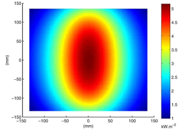
The equation 5 gives the illumination (W.m−2) of

differ-ential element of a plan illuminated by a cylinder. The cylinder have an isotropic luminance. The result is given on figure 5 for the conditions described in figure 3. The power P of the lamp is 1000 W.

The lamp radiates in all the space. To use the ray tracing method, we have to discretize the radiation of the lamp

Figure 4: Geometrical description of the cylinder-plate

Figure 5: Illumination of the square plate (W.m−2,

radios-ity)

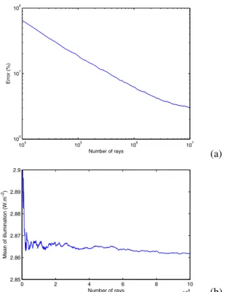
and define ray properties : departure, direction and ar-rival. We use the Monte Carlo’s method to define the ray departure and direction. We do not use regular discretiza-tion because the obtained result is discretizadiscretiza-tion depen-dent. With the Monte Carlo’s method we can control the error (ErF%, Eq.8) between the exact solution (Fig.7.a)

and thereby reduce calculating time. We can also control the convergence of the Monte Carlo’s solution by looking the evolution of the mean of the illumination of the plate (Fig.7.b). ErF% = 100 * + + + + , " -F_dradiosity₁₋₂ − Fdraytracing1−2 .2 dΩ " -F_dradiosity₁₋₂ .2dΩ (8) For 1.2 million of rays, the error between the solutions given by radiosity (Fig.5) and ray tracing (Fig.6) method is smaller than 5%. The calculating time is about 90s with an Intel Centrino CPU (2.6 GHz). The ray tracing method is validated in the case of a plate illuminated by one lamp. In the next section, we compare numerical results to ex-Integrated linear absorption coefficient

configuration −150 −100 −50 0 50 100 150 −150 −100 −50 0 50 100 150 (mm) (mm) 1 1.5 2 2.5 3 3.5 4 4.5 5 kW.m−2

Figure 6: Illumination of the square plate (W.m−2, ray

trac-ing)

Front face Rear face Air temperature 25◦C 25◦C

Convection coefficient 12 W.m−2.K 9 W.m−2.K Table 1: Simulated boundary conditions

perimental results and we propose a technique to reduce the calculating time in the case of 3D computation.

3 COMPARISON WITH EXPERIMENT

In this section we compare the results given by our ray tracing software, coupled with Comsol (FEM), to experi-mental results given in [3] for the heating stage of a rect-angular plate by an IR lamp (Fig.8).

In a first step, we compute the radiative source term (Eq.2), by using the ray tracing method, in all the plate (3D). Then, we use the result as an input data in a FEM software (here Comsol) to solve the heat balance equation (Eq.1). The figure 9 shows the source term for y= 0 in W.m−3. The radiation of the IR lamp is absorbed in few

µm in the plate. For the chosen example, the heating stage of the plate is in two steps: in first the face of the plate that is in front of the lamp is heated, during 65 s, then the lamp is turned off and the temperature, in the thickness, is ho-mogenised by conduction, during 25 s.

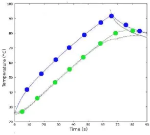
The figure 10 shows the evolution of the temperature in two points of the plate: one in the middle of the face that is in the front of the lamp (front face) and the second is at the opposite (rear face). On the same figure, there are the numerical and the experimental results. At the end of the heating stage (90 s) the difference between simulation and experimentation is lower than 5 %. The numerical results are the dotted line, the blue one is for the front face and the green one is for the rear face. The grey lines are for the experimental results. The boundary conditions used for the simulation are given in the table 1.

The computation time for this simulation is about 15 mn (Ray Tracing) for the source term and 3 mn (Comsol) for the temperature with a 2.6 Ghz CPU. The computation time of the source term is proportional to the number of

104 105 106 107 100 101 102 Number of rays Error (%) (a) 0 2 4 6 8 10 x 106 2.85 2.86 2.87 2.88 2.89 2.9 Number of rays Mean of illumination (W.m − 2) (b)

Figure 7: (a) Error between radiosity and ray tracing

meth-ods, (b) Convergence of the ray tracing method

lamps. In industrial oven you can have over 6 lamps and for this configuration the computation time is up to 1.5 hour. This time is acceptable for one simulation, but it can be unacceptable if you want to do an optimisation of the heating stage. In the next section we propose a technique to reduce the computation time for a lot of simulations.

4 TIME OPTIMISATION

In the simulation of the heating stage of a plate (or pre-form in a most general case), the calculation of the radia-tive source term is very time costly. In order to reduce the computing time cost, we propose to use interpolation

Figure 8: Experimental configuration

−150 −100 −50 0 50 100 150 −150 −100 −50 0 50 100 150 (mm) (mm) 1 1.5 2 2.5 3 3.5 4 4.5 5 kW.m−2

Figure 9: Radiative source term in the thickness (W.m−3)

Figure 10: Temperature evolution

for the calculation of the radiative source term. To realize this interpolation, we do a fixed number of direct calcula-tion of the source term (Fig.11). In our example, we can change the x and z position of the lamps. We discretize the plan (x,z) in 25 (5 on x axis and 5 on z axis) lamp po-sitions, and we create a data base of 25 radiative source terms . The calculation time is 5 hours for the 25 posi-tions. Now if you want to know the radiative source term for any x,z position of a lamp, you can use interpolation and the calculation time is reduced to 3 s.

We use theinterp2function in Matlab, with a cubic inter-polation, to realize the interpolation of the radiative source term. In order to validate this technique, we compare the result of a direct calculation and the result given by in-terpolation for arbitrary selected positions, in all our tests the error (ErQ%, Eq.9) between both results (Qinterpand

Qdirect) is under 3 %. So, with this technique the

calcula-tion time of the radiative source term comes from 15 mn to 3 s. ErQ% = 100 / " (Qinterp− Qdirect)2dΩ " (Qdirect)2dΩ (9)

Figure 11: Position of the lamps in the plan x,z

5 CONCLUSIONS

In this study we use the ray tracing method to compute the radiative source term used in the heat balance equa-tion. The ray tracing method is validated with two differ-ent ways : comparison with analytical solution and com-parison with experimental data. In both cases the error is lower than 5 %. The error can be controlled by using the Monte Carlo’s method.

We propose a simple technique to reduce the computation time cost of the ray tracing method in the case where we need a lot of iterations, like in optimisation of forming process. By using this technique, we introduce an error smaller than 3% and reduce the computation time from 15 mn to 3 s.

Next steps of this study are : the consideration of reflec-tors, the application to the heating stage of preform for the stretch blow moulding process.

ACKNOWLEDGEMENT

This research was supported by Toshiba Lighting France.

REFERENCES

[1] W. Cai.D´eveloppement et applications de mod`eles d’´echanges radiatifs par suivi de rayons. Th`ese de l’ ´Ecole des mines de Paris, in French, 1992. [2] M . Bellet F. M. Schmidt, J. F. Agassant.

Experimental study and numerical simulation of the injection stretch/blow molding process.POLYMER ENG. AND SC., 38:1399–1412, 1998.

[3] C. Champin.Mod´elisation 3D du chauffage par rayonnement infrarouge et de l’´etirage soufflage de corps creux en PET. Th`ese de l’ ´Ecole des mines de Paris, in French, 2007.

[4] R.A. Person H. Leuenberger. Compilation of radiation shape factors for cylindrical assemblies. ASME, 1956. 0 0.5 1 1.5 2 2.5 3 x 10−3 −0.1 −0.08 −0.06 −0.04 −0.02 0.02 0.04 0.06 0.08 0.1 m m 2 4 6 8 10 12 x 105 kW.m−3 0