HAL Id: hal-01636832
https://hal.archives-ouvertes.fr/hal-01636832
Submitted on 17 Nov 2017
HAL is a multi-disciplinary open access
archive for the deposit and dissemination of
sci-entific research documents, whether they are
pub-lished or not. The documents may come from
teaching and research institutions in France or
abroad, or from public or private research centers.
L’archive ouverte pluridisciplinaire HAL, est
destinée au dépôt et à la diffusion de documents
scientifiques de niveau recherche, publiés ou non,
émanant des établissements d’enseignement et de
recherche français ou étrangers, des laboratoires
publics ou privés.
Shape distortions induced by convective effect on hot
object in visible, near infrared and infrared bands
Anthony Delmas, Yannick Le Maoult, Jean-Marie Buchlin, Thierry Sentenac,
Jean-José Orteu
To cite this version:
Anthony Delmas, Yannick Le Maoult, Jean-Marie Buchlin, Thierry Sentenac, Jean-José Orteu. Shape
distortions induced by convective effect on hot object in visible, near infrared and infrared bands.
Experiments in Fluids, Springer Verlag (Germany), 2013, 54 (4), pp.1452.
�10.1007/s00348-012-1452-8�. �hal-01636832�
Shape distortions induced by convective effect on hot object
in visible, near infrared and infrared bands
Anthony Delmas •Yannick Le Maoult• Jean-Marie Buchlin•Thierry Sentenac• Jean-Jose´ Orteu
Abstract The goal of this study is to examine the per turbation induced by the convective effect (or mirage effect) on shape measurement and to give an estimation of the error induced. This work explores the mirage effect in different spectral bands and single wavelengths. A numerical approach is adopted and an original setup has been devel oped in order to investigate easily all the spectral bands of interest with the help of a CCD camera (Si, 0.35 1.1lm), a near infrared camera (VisGaAs, 0.8 1.7lm) or infrared cameras (8 12lm). Displacements due to the perturbation for each spectral band are measured and finally some hints about how to correct them are given.
1 Introduction
In industry and in research laboratories, it is often necessary to conduct non contact measurements of temperature and/or size on hot objects. A good way to do this is to use cameras and to observe the object of which we want to know the size (or displacements if a load is applied) and temperature. Some studies have been carried out on the use of common visible CCD cameras (Silicium detector 0.35 1.1lm) to make ther mal dimensional coupled measurements and merge usual video data with infrared data (Healey and Kondepudy1994). There are several advantages to working in the near infrared
band when measuring temperature:high sensitivity, good detector resolution, and a system less dependent on the unknown emissivity of metals (Herve et al.1997). However, some investigations (Claudinon 2000) made in this specific domain have revealed some perturbations at high temperature ðT " 800#CÞ, with the standard deviation of dimensional
measurements being multiplied by 5. Numerous works carried out using cameras to provide measurements have pointed out the problem of images perturbed by the refractive index gra dient in the air (Bing et al. 2010; De Strycker et al. 2010; Lyons et al.1996; Grant et al.2009). In this study, we shall focus on perturbations which arise from the convective effect present around hot objects. Such perturbations can induce an image distortion in the visible band but also errors on shape and temperature measurements for near infrared and infrared bands. We chose first to focus on simple geometry objects like a cylinder or a hot horizontal disk, in order to generate a reproducible convective plume. We present here a numerical way [ray tracing method (Cosson et al. 2011)] to obtain the displacement induced by the density variation and an experi mental approach to obtain quantitative values of displace ments. Because of the recent emergence of new generation cameras with high resolution, even in the infrared band, this experimental method is carried out for several spectral bands going from visible to infrared. Finally, we suggest some prospects about a strategy for correcting perturbed images.
2 Background on mirage effect: description, generation, and convective flow
2.1 Mirage effect
The mirage effect appears as soon as a refractive gradient is present. What we call a mirage effect is when light beams
A. Delmas (&) Y. L. Maoult T. Sentenac J. J. Orteu Institut Cle´ment Ader, Universite´ de Toulouse, Mines Albi, Campus Jarlard, Route de Teillet, Albi 81013, France e mail: adelmas@mines albi.fr
J. M. Buchlin
Environmental and Applied Fluid Dynamics Department, Von Karman Institute, 72 Chausse de Waterloo, Rhode St Gene`se 1640, Belgium
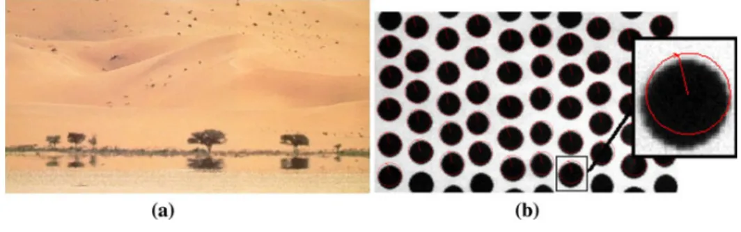
do not arrive at the expected destination, that is, to say without temperature gradient. Usually, this effect does not have a big influence on optical measurement. But, in the presence of a strong refractive index gradient, the infor mation measured can go through a large distortion. In our case, the refractive gradient is engendered by a temperature gradient coming from a natural convective plume. The convection is induced by the movement of molecules within fluids, here, the air, due to temperature differences which affect the density, and thus the relative buoyancy, of the fluid. More dense components will fall while less dense components rise, leading to bulk fluid movement. In the case of a hot object, the convective field around it will generate the temperature gradient around the object. This temperature gradient around and above the object provides a refractive index gradient which, if the deviation is big enough, can produce large aberrations. Light distortions induced by natural convection are very frequent and can be observed in numerous cases. The best known is the mirage effect, which occurs over a road or in the desert when the sun is strongly hitting the ground.
Either the observed object is far away (hundreds of meters) and the deflection can be important even with small gradient (20#C of relative difference) or the object is close
to the observer (a few meters or centimeters) but the temperature gradient is much stronger (500#C to ambient temperature) (Fig.1). Moreover, an important part of the mirage effect, especially in distant observations such as astronomical cases, is flicker due to turbulence and slow large scale instabilities.
Here, we shall consider a mirage effect occurring within a short distance. This can sometimes be a real problem when it is necessary to know with accuracy the shape or the temperature of a given point of the object. The error made in such attempts at dimensional measurement is given in this work. In addition, the deflection induced by the tem perature gradient varies with the wavelength. According to Eq.(1) called the Gladstone Dale law (Mayinger and Feldmann 2001), it is possible, for a given temperature field and wavelength, to obtain the refractive index distribution.
nk& 1 ¼ Kk% qðTÞ ð1Þ
where
Kk¼ ðN % a0Þ=ð2 % !0Þ ðm3kg 1Þ ð2Þ
The Gladstone Dale parameter K is a function of the wavelength k (because a0: polarizability of one molecule
depends on kÞ; !0 is the vacuum permittivity, and N is the
Avogadro number. We have chosen to work first in the visible band, with the wavelength of the He Ne laser: k = 632.8 nm and K = 0,2256 9 10- 3m3 kg-1.
And for the densityq(T), the air can be taken as an ideal gas:
qðTÞ ¼ ðP % MÞ=ðR % TÞ ðkg m 3
Þ ð3Þ
Withq the density (kg m-3), P the pressure (Pa), M the
molecular mass (kg), R the perfect gas constant, T the temperature (K), and so:
qðTÞ ¼ 352:86=T ðkg m 3
Þ ð4Þ
Finally, by combining Eqs. (1) and (3), it is possible to establish, for the specific wavelength of an He Ne laser: n & 1 ¼ 0:079=T ð5Þ
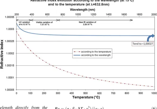
Figure2shows how the refractive index depends on the temperature and on the wavelength. The index of refraction decreases with the rise in temperature or wavelength. The variation in the refractive index is highest for the short wavelengths (ultraviolet and visible). However, this variation quickly tends to a constant value as the wavelength increases. Knowing that the bigger the refractive index is, the more the light is deviated, if a mirage effect is observed with a visible camera (or with the naked eye), the biggest deviation corresponds to the shortest wavelength of the camera (&400 nm). This means that it is not necessary to use an effective refractive index for a spectral band (refractive index integrated index over the spectral band) to obtain the displacement observed, but only that corresponding to the shortest wavelength. Above 1,000 nm, it does not really matter any more since the refractive index varies only very slightly. It is now possible to obtain the refractive index
Fig. 1 a Mirage effect with distant objects, b mirage effect with object 1 m away (circles are the original shape of the black disks)
distribution for a given wavelength directly from the temperature field (conf. Eq.1).
2.2 Convective flow and choice of the perturbation geometry
The next step is to choose a hot object able to generate a reproducible convective effect with an high temperature and refractive index field. The choice of a vertical hot plate leads to some problems obtaining good temperature homogeneity across the plate and the generation of a sta bilized boundary layer (Crespy2009). Moreover, this kind of perturbation is very close to a 1D effect and thus gen erates a weak light deviation. We finally settled on the creation of a plume coming from a hot horizontal disk. Generating the perturbation in this way is appropriate for our needs because it is a free convection, in agreement with our context, and in addition, such a system allows us to obtain both a strong displacement of the lights through the perturbation and a heating element of small dimensions.
The expected displacements and the size of the heating element were both validated using a ray tracing method and a computational fluid dynamics (CFD) software (cf. Sect. 3). Furthermore, since the heating element is much smaller than a vertical plate, it is possible to generate very high temperature with good homogeneity. The next section explains how the design of the setup was selected.
The heating element chosen was a hot horizontal disk generating an axisymmetric plume. We discuss here the diameter and temperature range necessary to provide a displacement big enough to be measured. In free convec tion, a non dimensional number is used as a reference to predict the flow regime; this is the Rayleigh number:
Ra ¼ ðg % b % DT % x3
Þ=ða % mÞ ð6Þ
With g the gravitational acceleration, b the dilatation coefficient,DT the difference of temperature between the air and the disk, x the characteristic length (diameter of the disk), a the thermal diffusivity of the air, and m the kinematic viscosity. As said previously, it was necessary to use a small enough object that could be easily heated up and which had good surface homogeneity. For example, for a disk with a diameter of 10 cm, heated up to 1,200 K (around the highest temperature of materials encountered in our laboratory) the Rayleigh number is equal to 2.19 9 106. This means that the flow will never reach a turbulent regime because the transition limit between laminar and turbulence appears at Ra = 109. With this type of laminar plume, the flow is easily reproducible and well established. We can notice here that this laminar convective flow corresponds to most of the hot objects studied in the laboratory (image averaging may be required in order to override external perturbations). In addition, the big advantage of a perturbation generated by such a setup is the displacement brought through the plume. Indeed, an axisymmetric perturbation brings, just by its own curved shape, a light deviation. Moreover, the temperature gradient in the plume is very strong (much stronger for example than a jet of hot air blowing from a pipe) and thus gives another way to deviate the rays of light efficiently.
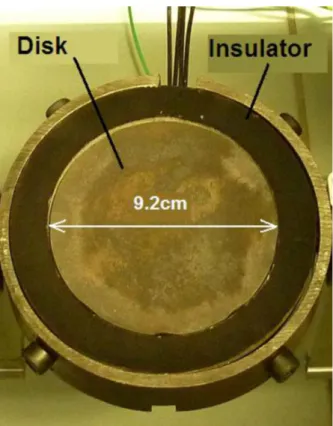
The chosen geometry is therefore a heated disk giving a steady laminar flow with a strong temperature gradient and thus, a perturbation inducing a deviation of the rays. Figure3 shows the disk used for the experimental method. More details about it will be given in the Sect.3.3.
Fig. 2 Refractive index evolution according to the wavelength (at 15#C) and to the temperature (atk = 632.8 nm) (Lide2007)
3 Numerical tools
This section deals with the numerical simulation of the deflection induced by the plume. Our numerical approach is described briefly in Fig. 4.
The first step is to obtain the temperature field above the disk. This input data are computed with a CFD software. The next step is to deduce the refractive index (using the Gladstone Dale law: Eq. 1) from the temperature field and to include it in the ray tracing code. This allows us to have a whole numerical approach giving as a final result the displacement field induced by the convective plume. In addition, an insulator was taken into account in the simu lation in order to avoid a temperature gradient on the disk surface during the experiment.
3.1 Computational fluid dynamics (CFD)
For this CFD study, Fluent was chosen, because of its good performance in solving energy and movement equations.
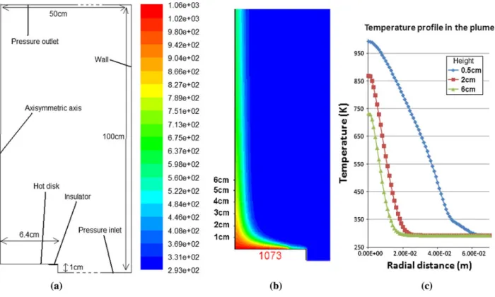
The axisymmetric geometry is meshed with Gambit and then introduced into Fluent (Fig.5). The size of the domain needs to be big enough (50 cm 9 100 cm) to avoid any kind of border effect. The mesh was made in such a way as to obtain smaller cells close to the disk. The number of cells in this simulation was 60,000 (300 vertically by 200 horizontally). As has been mentioned, the computation was carried out in laminar flow. Different correlations were used to define the air properties in the range of 300 1,300 K (El Motassadeq et al.2000).
As regards the density, the air can be assimilated as a perfect gas (cf. Eq.4). The error made compared to the exact values were, on average, about 0.16 % in our tem perature range (300 1,300 K). In these conditions, we obtained the temperature field around and above the disk (Fig.5).
The temperature field obtained is the input data to obtain the refractive index field. The validation of the Fluent results will be described in Sect.4and numerical results will be compared to the experimental ones.
3.2 Ray tracing
The ray tracing code was initially developed to simulate the heating of plastic preform at the Institut Cle´ment Ader laboratory (Cosson et al.2011). The code has been modi fied for our study to be able to make optic computations in an environment of inhomogeneous refractive indexes. 3.2.1 Validation
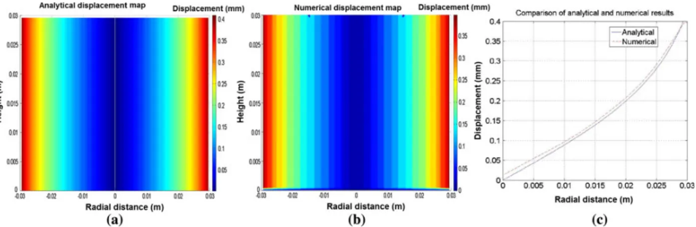
To validate the ray tracing code in this particular new configuration, we chose to compare analytical results with numerical ones, as the code was modified for our mirage effect case. In order to obtain easily analyzable results, a simplified geometry was used. This geometry, used to compute the displacement in a cylinder analytically, is shown in Fig.6. The cylinder contains two layers of dif ferent refractive indexes itself in a third medium (index0 = 1.0003, index1 = 1.0002, index2 = 1.0001).
The same geometry as that used for the ray tracing code was built. To compare the results more easily, the dis cretization has, in both cases, a horizontal node number of 120 points equally distributed at 3 cm to the right and left of the axis of the cylinder. Figure7shows the comparison between analytical and ray tracing (numerical) results. The results obtained are in good agreement (a mean relative error of 3 %). However, it is important to keep in mind that the numerical results will depend strongly on the meshing realized for the refractive index field. This meshing can be adjusted using three discretization parameters: along the radius, the height, and the circumference. We do not give much detail in this paper about the parametric analysis but
Fig. 3 Photograph of the disk used for the experimental method
we conclude by saying that the refractive index gradient being essentially horizontal and for a field having an axi symmetrical shape, the key parameter will be the circum ference discretization. The Fig.7b shows clearly that the displacement values of the numerical results are less nuanced. This is directly linked to the circumference dis cretization. A large number of nodes (used for the meshing) along this direction can solve this problem easily. As result, a minimum number of 100 nodes along the circumference was used in our computation. Figure7c illustrates the displacement obtained by analytical computation and the ray tracing method and shows the good agreement between both methods (with a mean error of 2 %).
After this validation step, the ray tracing code can be used to compute quantitative displacement induced by the plume above the disk.
3.2.2 Simulation
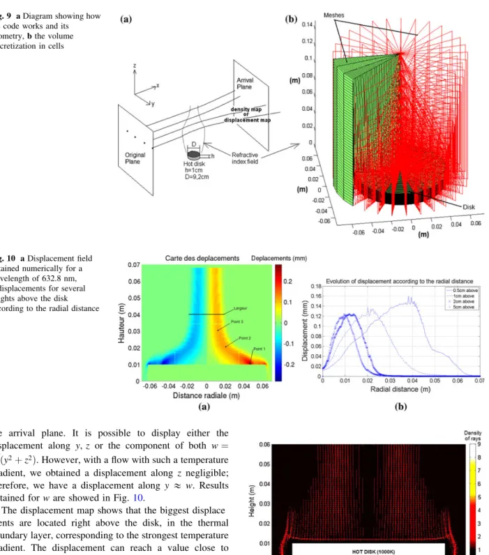
For the input data of the code, the Gladstone Dale law (Eq. 5) is used to deduce, from the temperature of the plume, the refractive index field for a given wavelength (for the example k = 632.8 nm). Finally, this refractive index field is incorporated in our ray tracing code as shown in Fig.9. The original plane is composed of radiating elements located with their y and z coordinates. Each
Fig. 5 a Mesh and boundary conditions used with Fluent, b temperature field obtained with Fluent and c Temperature profiles for different heights in the plume
Fig. 6 a Geometry and distances used for the validation, b illustration of angles used for the analytical calculation
element launches one ray perpendicularly to the original plane. The refractive index field around and above the disk is discretized according to the radial, circumferential, and axial coordinates in order to create a large number of cells with a constant refractive index (Fig.9).
A parametrical analysis on the mesh was carried out in order to obtain accurate results within a reasonable time frame (the creation of 1,000,000 cells (100 9 100 9 100) leads to several days of computation [15 days on our computer: AMD Opterion 2 GHz, 1 Mo cache, 2 GB Ram, on Linux Feodora]). For this reason, an optimized meshing was used for our model in accordance with the parametric analysis (cf. remarks made in Sect.3.2.1). A discretization of 20 along the height, 50 along the radius and 110 for the circumference, that is to say 110,000 cells in total, were used; the computing time was approximately 3 h. The error between a meshing of 1,000,000 cells and a meshing of 50,000 cells was lower than 5 %. Figure8 shows the evolution of the meshing time and the relative error between the reference mesh (100 9 100 9 100) and the other mesh. We can clearly see the good precision and the time saving obtained with the optimized mesh (20 9 50 9 110). However, if we keep such discretization, and because the rays are launched normal to the original plane (cf. Fig.9a), it is not possible to obtain a vertical displacement. That is why, a fourth discretization is done in order to create, where the gradient of the refractive index is not aligned with the mesh, cell surfaces with a better alignment with the gradient.
The transition from one cell to another is governed by Snell Descartes’s law (transition between a cell i to a cell j with n and h, respectively, the refractive index of the cell and the angle between the ray and the normal to the cell surface):
ni% sinðhiÞ ¼ nj% sinðhjÞ ð7Þ
Then, when the ray goes out of the last cell, thus leaving the thermal perturbation, it continues its path until the
arrival plane, whose position according to x can be adjusted to accentuate the distortion effect. Indeed, the further away the screen is, the higher the deviation. In our example, a distance of 37 cm was chosen. If the original plane is sufficiently discretized and thus enough rays are launched (around 500,000 to obtain Fig.10), a displacement map is obtained on the arrival plane. The most important aspect is to discretize the arrival plane sufficiently because this will directly affect the accuracy of the displacement. For example, if the arrival plane size is 7 cm 9 7 cm, and if we discretize it by 1,000 9 1,000, the smallest displacement measurable is 0.07 mm. But by using mathematical interpolation, it is possible to reach a much smaller displacement. The discretization of the original plane matters mainly in terms of visualization of the results. Indeed, this discretization will directly define the matrix size on the arrival plane since the discretization of the original plane fixes the number of rays launched. The displacement map obtained makes possible to quantify the displacement of each ray between the starting plane and
Fig. 7 a Analytical results, b numerical results (obtained with (120 rays horizontally), c comparison of analytical and numerical result
Fig. 8 Evolution of the relative error and meshing time according to the mesh dimensions
the arrival plane. It is possible to display either the displacement along y, z or the component of both w¼
ðy2þ z2Þ
p
. However, with a flow with such a temperature gradient, we obtained a displacement along z negligible; therefore, we have a displacement along y& w. Results obtained for w are showed in Fig.10.
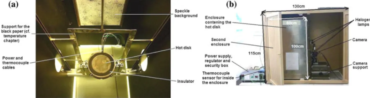
The displacement map shows that the biggest displace ments are located right above the disk, in the thermal boundary layer, corresponding to the strongest temperature gradient. The displacement can reach a value close to 0.3 mm above the disk and 0.13 mm in the plume. In agreement with Snell Descartes’s law, there are no dis placements in the center of the plume. The points used to read the displacement on the map and the plume width are located in Fig.10.
The ray tracing code also makes it possible to obtain a density map on the arrival plane which shows convergence zones of rays or alternatively, dark zones, corresponding to regions where few or no rays arrive. Figure11provides an
example of results obtained for the case where the disk is heated at 1,073 K without insulator, with the arrival plane located 5 m behind the center of the disk and for the spe cific wavelength of the He Ne laser (k = 632.8 nm).
Fig. 9 a Diagram showing how the code works and its geometry, b the volume discretization in cells
Fig. 10 a Displacement field obtained numerically for a wavelength of 632.8 nm, b displacements for several heights above the disk according to the radial distance
Because the hot object is uninsulated and observed from a distance, this case could illustrate a classical example of a practical industrial situation. It shows the distortion effect: every ray passing near the vertical edge of the disk goes toward the colder temperatures (higher refractive index) creating the dark zone. Consequently, a convergent zone (clearer area) corresponds to rays missing in the dark zone. This means that if one is looking at the shadow of the disk with a technique such as schlieren photography or shad owgraphy, this whole dark zone will not be due to the disk itself but to the mirage effect as well. This property of the mirage effect can be used to hide objects (Aliev et al.
2011), especially in fluids, such as water, with high refractive index variations with temperature.
The numerical steps described in this chapter provided all the information needed to select the proper setup: an apparatus able to generate a convective and reproducible plume inducing a displacement large enough to be mea sured by mean of cameras. In the next section, we shall describe the experimental setup used in our study. 3.3 Experimental setup design
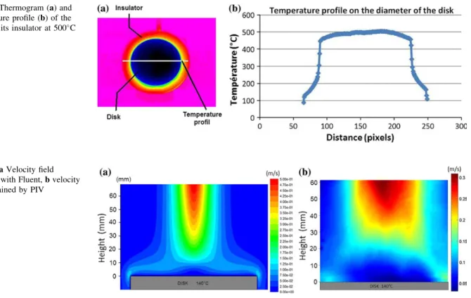
The disk selected for the experiment has a diameter of 9.2 cm with 1 cm of thickness. It is made of Inconel 600 and is heated up using a resistance coiled and welded under it. The maximum temperature reachable (so as not to deteriorate the welds) is 1,200 K with a power heating of 1,300 W. The heating element includes two embedded thermocouples used for regulation and security. The disk is surrounded with an insulator made of mica paper impreg nated with silicone resin under high pressure and temper ature. This material has a poor conductivity (0.27 W m-1K-1) and can easily resist high temperature up to 1,073 K. To avoid any perturbations coming from the surrounding environment, an enclosure is needed. We chose to construct an enclosure with metallic plates painted in black in order to avoid reflections on the walls (Fig.12). Different holes were made on its sides for future experi ments. Figure12 shows that the whole enclosure is
included in a second enclosure made of wood to avoid again perturbation coming from the room. The plume is very sensitive to the outcoming variation of pressure. In fact, the pressure variation in the plume is extremely small, around 1 or 2 Pa only (Crespy2009).
4 Characterization and tests of the experimental setup 4.1 Characterization of the disk
The first test performed on the disk was done to verify the stability of the temperature and its homogeneity on the disk surface. In order to regulate the disk and to supply it with power, a PID regulator and a power supply unit were used (Fig.12). A black paint for high temperature was applied on the surface in order to give uniform emissivity (e ¼ 0:91) and to enable observation with an infrared camera during the heating period (Fig.13). The tempera ture of the resistance was set at 1,073 K. The heating element reached stability (within 0.1 K) after a slow increase in the temperature (20 K per min). The mean surface temperature was given by the camera and was equal to 1,073 K with a standard deviation of 18.4 K (if a smaller zone of interest is taken rather than the whole disk, a much smaller standard deviation is obtained).
The surface of the disk is therefore homogeneous at 2.3 %. The next part of the paper describes the character ization of the hot plume generated by this device. The main parameters needed to characterize this perturbation (hot plume) are the velocity and the temperature fields inside the plume. These key parameters are needed to validate the CFD step.
4.2 Plume characterization 4.2.1 Velocity in the plume
To study the velocity of the hot air in the plume with accuracy, a PIV (Particle Image Velocimetry) method
(Scarano et al. 2000) combined with a LDV (Laser Doppler Velocimetry) (Riethmuller and Tomita 1987) method was used (first step of Fluent validation).
For this experiment, a special enclosure in plexiglass was built in order to allow the laser light scattered by the particles to reach the camera. Indeed, no holes were made on the enclosure to give the most homogeneous seeding. The seeding used in our case of natural convective flow was oil smoke generated by spraying some oil drops on a hot plate (450 K). The size of particles obtained was around 3lm. The laser sheet was located in the center of the disk in order to have a velocity field comparable to that obtained with Fluent. The PCO Sensicam camera used has a sensor of 1, 280 9 1, 024 which allows us, when coupled with a lens of 55 mm focal length, to obtain a spatial resolution on the laser sheet of 0.08 mm and to explore an area of 8.2 cm 9 10.2 cm. The velocity fields obtained with the PIV are shown in Fig.14 (averaged over 30 pictures).
The values found in the middle of the plume at 6 cm above the disk were 0.32 and 0.475 m/s, respectively, for the experimental and numerical results. The lower speed for the experimental result can be explained by the fact that an average image is considered. Indeed, the convective plume was actually not as stable as had been imagined, which means that the maximum velocity is not always located exactly at the same place. Hence, the average over
30 images decrease the values issued from an instantaneous image. The average of the maximums of each picture gives a speed of 0.47 m/s which is in very good agreement with Fluent results (error\1 %). The resulting image (Fig.14), obtained by applying an average, shows that the shape of the velocity field is similar.
The LDV uses the same seeding as the PIV but the difference here is that the measurement is not 2D but 1D. This allows us to obtain the velocity of the plume very locally. The particles are illuminated by a known wave length of laser light (632.8 nm). The scattered light is detected by a photomultiplier tube, an instrument that generates a current related to absorbed photon energy and then amplifies that current. The difference between the incident and scattered light frequencies is called the Doppler shift. By analyzing the Doppler equivalent fre quency of the laser light scattered (intensity modulations within the crossed beam probe volume) by the seeded particles within the flow, the local velocity of the fluid can be determined.
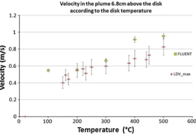
We chose to measure the velocity in the center of the plume 6.8 cm above the disk for different disk tempera tures and to compare it to Fluent. The results are in fair agreement (Fig. 15) with the numerical result (with a mean error around 10 %). As for the PIV, LDV results should not be averaged if we want to keep the real physical signifi cance of the velocity. With this aim, we simply took
Fig. 13 Thermogram (a) and temperature profile (b) of the disk and its insulator at 500#C
Fig. 14 a Velocity field obtained with Fluent, b velocity field obtained by PIV
acquisition of few seconds for each disk temperature and kept only the maximum value.
4.2.2 Temperature in the plume
The plume obtained with this heating element was inves tigated by means of the specific method of infrared ther mography and was compared to results obtained with Fluent. This technique directly gives us the 2D temperature field inside the plume. First, we placed vertically, in the middle of the plume, a sheet of paper coated with a black paint (of known emissivity, e ¼ 0:91) and then measured the temperature taken by the paper itself. The temperature of the disk was fixed at 100#C (373K). The numerical and experimental temperature fields are shown, and a profile at a given height (20 mm above the disk) is compared to a Fluent profile in Fig.16.
To find out whether the paper can be considered as a thermally thin object, the Biot number needs to be used and is defined by Bi¼h:L
k with h the convective coefficient,
L the thickness of the paper, and k its thermal conductivity.
After obtaining the thermal properties of this paper (k& 0.14 W m-1K-1and L = 150
lm), we computed a representative h with the help of Fluent results (h = 25 W m-2K-1). The Biot number found for the paper is &0.03 \ 0.1; it is known in thermal studies that such a Biot number leads to a thermally thin object which means that the paper will take, in all its depth, the temperature of the fluid in contact. However, we can see in Fig.16that the width of the experimental plume is slightly longer than the width of the numerical plume. There could be several reasons for this phenomenon:
• First, the lateral diffusion in the paper can lead to a plume with more width and thus a maximum temper ature that is lower. However, according to our calcu lations, the diffusion length is only around a few millimeters, so this does not seem to be the main reason.
• Moreover, if the paper is not situated exactly in the middle of the plume, few degrees can easily be lost (around 10 K within 5 mm).
• And finally, the plume itself could be slightly larger than the size given by Fluent or could move slightly from left to right, creating a wider plume on the paper. This phenomenon of fluctuation in a convective flow, despite the presence of an enclosure, has been pointed out in another study (Bruce 2011). With the aim of observing the plume precisely, to see the movement in the flow, schlieren photography was carried out (cf. Sect. 4.2.3).
4.2.3 Schlieren photography
Due to drawbacks seen in the previous section, the char acterization of the shape of the plume was combined with a schlieren photography technique. Schlieren photography is a visual process that is used to photograph fluid flows of varying density. The basic optical schlieren system uses
Fig. 15 Comparison between measured (LDV) and predicted plume velocity versus disk temperature
Fig. 16 a Temperature field obtained with Fluent, b temperature field obtained with the infrared camera, c temperature profiles 20 mm above the disk obtained experimentally and numerically
light from a single collimated source lighting on a target object. Variations in refractive index caused by density gradients in the fluid distort the collimated light beam. The collimated light is focused with a lens, and a knife edge is placed at the focal point, positioned to block about half of the light. In a flow with uniform density, this will simply make the photograph half as bright. However, in a flow with density variations, the distorted beams focus imper fectly and parts which have been focused in an area cov ered by the knife edge are blocked. The result is a set of lighter and darker patches corresponding to positive and negative fluid density gradients in the direction normal to the knife edge.
Several interference filters (centered on 429, 530, 650 nm) were used in our experiment to see whether it was possible to distinguish an enlargement of the diameter between several wavelengths (cf Fig. 2) and then to com pare it with that calculated with ray tracing (Table1). But
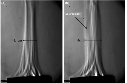
as can be seen in this table, the width changes only by 0.8 mm in the visible band, which is too small to be clearly seen by the schlieren photography technique. Nevertheless, if we check the average width of the plume itself over the different wavelengths with the numerical results, we find a length in agreement with the error of a few percent given by the numerical results. If undisturbed, the plume is a steady flow whose energy transport rate is equal to the heat transfer rate from the disk surface. Theoretically, the plume width (at a given elevation) should decrease with increased source strength (Robinson and Liburdy1987). In practice, the plume always moves a little (a few millimeters at low temperatures up to a few centimeters at high temperatures); it is then very sensitive to the surroundings and it is very hard, almost impossible, to keep a steady flow above 750 or 800 K. This could explain why the plume seems a little wider in the thermographic measurements. An example of the images taken with this method is shown in Fig.17.
Table 1 Displacements expected for each wavelength and width of the plume
Type of cameras UV camera Classical camera CCD NIR IR
Resolution 1,388 9 1,038 320 9 256 320 9 240
Wavelengths 200 nm 400 nm 632.8 nm 750 nm 1lm 8lm
Maximum displacement above the disk: point 1 (mm) 0.323 0.2822 0.2761 0.2751 0.2739 0.2705
Maximum displacement in the plume: point 2 (mm) 0.1542 0.1274 0.1246 0.1242 0.1236 0.1221
Maximum displacement in the plume: point 3 (mm) 0.1457 0.1271 0.1244 0.1239 0.1234 0.1218
Plume width 3 cm above the disk (mm) 43.00 42.34 42.28 42.26 42.24 42.18
Fig. 17 Image of the plume taken with the Schlieren photography technique (disk temperature = 770 K) without fluctuations (a) and with fluctuations (b)
As a conclusion to this Sect.3.3, we have shown that there is a fair agreement between Fluent computations and the experiments. In the next section, the numerical results of ray tracing will be compared with experimental dis placement results.
5 Displacements results
To measure the displacements induced by the plume, a technique called ‘‘Background Oriented Schlieren’’ (BOS) (Klinge2001) was used. Background Oriented Schlieren is a technique for flow visualization of density gradients in fluids using the Gladstone Dale relation between density and refractive index of the fluid. BOS simplifies the visu alization process by eliminating the need for expensive mirrors, lasers, and knife edges. In its simplest form, BOS makes use of simple background patterns of randomly generated dots. In its initial stages of implementation, it was mostly being used as a qualitative visualization method. But in our case, thanks to a correlation software, it is possible to obtain a quantitative displacement field. Figure 18gives the principles of the BOS method.
To obtain results for displacement, two images of the background were recorded, one with perturbation and one without. Then, an analysis of these images was made in order to deduce the displacement of each element from the dot pattern. This analysis was carried out with the help of the software VIC2D (VIC 2D). The software makes a correlation between the two images and gives the dis placement in pixels of each element along the x direction
and y direction (displacement field). Since the background is made of black dots randomly distributed and because each dot is bigger than 1 pixel, we are able to obtain subpixel displacement. The displacement measured by the camera is directly linked to its distance from the plume. The distance Z is fixed at 30 cm and P1I at 67 cm (cf Fig.18). The BOS was performed for different ranges of wavelength (visible, near infrared, and infrared).
6 Result in the visible band
The camera used here was a Pike F 145B/C with Sony ICX285 CCD sensor. The sensor resolution was 1,388 9 1,038, which works efficiently between 400 and 800 nm. We used a lens with a focal length of 35 mm which allowed us to explore around 7.5 cm width in the plume a few millimeters above the disk. With such a setup and with a disk heated up to 800#C, we obtained the fol
lowing displacement field (Fig.19):
Figure19 shows the perturbation produced by the presence of the plume created by the hot disk. As expected, a deviation of rays of light occurs on the right side (dis placement in the x direction) and left side (displacement inverse to the x direction) of the plume, whereas the center of the plume keeps a displacement very close to 0. If the mean of the maximum displacement over all the pictures taken (600) is computed, we obtain a displacement of 0.225 mm which is in good agreement with the numerical result (Table 1) considering that the maximum displace ment is located between points 1 and 2 (Fig.10). The difference between the numerical and experimental results is lower than 10 %.
6.1 Result in the near infrared band
For the near infrared band, we used a XenICs camera XEVA FOA 1.7 320. with a VisGaAs sensor. This sensor of 320 9 256 works exceptionally well in the range of 400 1,700 nm. We had to insert a filter between the lens and the density variation in order to cut off the visible
Fig. 18 Diagram explaining the BOS technique
Fig. 19 a Field of view of the camera, b displacement field in visible band (averaged over 20 images)
spectral band. The filter from Optosigma company cuts 100 % of rays under 850 nm. The focal length of the lens used in this case, because of the lower resolution, is 50 mm, which gives 6 cm of the plume in the field of view. The zone of interest in pixels is 290 9 225 (Fig.20).
As shown in Fig.20, we can still locate the center of the plume between the two zones of positive and negative displacements (red and blue). The lowest displacement higher up in the plume does not appear clearly with such a camera because of the weak resolution of the sensor (even though we used a longer focal length). But we can still easily distinguish the perturbation occurring close to the disk. The two bottom corners of the figure have to be ignored because of correlation problems in this zone, as well as some blue and red ‘‘points’’ in the plume, corre sponding to dead pixels. If we compute the average of the maximum displacement over 600 pictures, we obtain a value of 0.24 mm. This result is in fair agreement with the numerical result, with 12 % difference.
6.2 Result in the infrared band
For the infrared measurement, we used a FLIR SC325 camera. The microbolometric sensor working between 7.5 and 13.5lm (and &20#C up to ?700#C) had a resolution
of 320 9 240 pixels. The lens used for the experiment had
a focal length of 30 mm, giving us the possibility to have 10 cm (width) of field of view in the plume. The back ground observed with the camera in this case was different than before. We created an IR pattern (Saint Laurent et al.
2010) using a copper plate painted in black and heated () 250#C) by a MICA resistance, and an aluminum plate pierced with holes (Fig.21). The pattern is smaller than the field of view of the camera (too short a focal length or too small a pattern) and that is why Fig.22 shows only a matrix of 175 9 140.
As might be supposed, the density results with such a pattern are inferior to those obtained with previous back grounds. Nevertheless, thanks to the interpolations made by the software VIC2D, we can obtain a similar result. We notice, however, some vertical bands on the pictures which actually correspond to zones without holes. We see in Fig.22 a part of the plume with no displacement in the center and, respectively, a positive and negative displace ment on the right and left side of the plume. The dis placement is slightly lower than in the previous case because the picture was taken a little higher up in the plume (see Fig.22). Indeed, the contrast at the bottom of the pattern decreased with time because of the disk radia tion heating the bottom of the aluminum plate. The average maximum displacement computed here was 0.15 mm, still in agreement with the numerical results obtained in the
Fig. 20 a Field of view of the camera, b displacement field in near infrared band (averaged over 10 images)
plume. The two dark ‘‘points’’ on the picture correspond to the screws used to hold the aluminum plate with the heating element.
All the experimental results obtained in the three spec tral bands are summarised in Table2
7 Conclusion, discussion and perspectives
This work has pointed out the mirage effect phenomena in several spectral bands and has provided quantitative information about the displacement induced by the per turbation. We showed, thanks to an original setup allowing measurement in all the camera spectral bands, that the displacement was around 0.26 mm close to the disk and about half that amount in the plume. The variation of the refractive index is essentially due to the temperature gra dient (compared to the wavelength) and thus the dis placements observed in any spectral bands are almost the same. The difference in displacement between the bands comes from the difference in resolution. Indeed, we show that the maximum difference between 400 nm and 8lm is only 4 %. The main problem with the experimental results in the near infrared and infrared spectral bands compared to the visible is the significant difference in the sensor reso lution. The camera has to be far enough away from the perturbation (or a longer focal length should be used) to allow a measurement of the displacement. In our case, a strong temperature gradient and a sufficiently long focal
length gave us interesting results. We also show that the displacement generated by the axisymmetric plume was predictable by our ray tracing tool (and by the preliminary use of a CFD software). Many experiments have been carried out in order to validate the numerical method, such as infrared thermography, particle image velocimetry, laser doppler velocimetry or schlieren photography. All the experiments were in good agreement with the Fluent results, and indeed the final measurements with back ground oriented schlieren support the accuracy of the numerical method.
However, as it has been described in this paper, the fluctuations of the plume lead to some small divergences between numerical and experimental results. In order to improve the stability of the flow more, one of the reviewers of this work has suggested to place a cone in the center of the plate, which was tested and found to work for modest temperatures only. The Fig. 23 shows instantaneous dis placement fields above the disk at different temperatures with a cone of 2 cm high and 2 cm wide.
Unfortunately, as we can see, the flow remains stable only at a disk temperature lower than 573 K beside the improvement brought to the setup. A whole new setup or flow generation could be investigated to create a stabilized perturbation.
Then, the next work will be to use this numerical method (developed in this paper) to estimate the error made in the temperature measurement because of the presence of the hot plume. This error could be induced by the
Fig. 22 a Field of view of the camera, b displacement field in infrared band (averaged over 10 images)
Table 2 Summary of displacements found
experimentally and numerically for each spectral band (for the point location: cf. Fig.10)
Type of cameras Camera CCD visible Camera NIR Camera IR
Resolution 1,388 9 1,038 320 9 256 320 9 240
Spectral bands 400 750 nm 850 nm 1.7lm 7.5 13.5 lm
Maximum displacement numerically(mm) point 1 0.282 0.274 0.271
Maximum displacement numerically(mm) point 2 0.127 0.124 0.122
Maximum displacement numerically(mm) point 3 0.127 0.123 0.122
displacement of the hot points from the background and to the convergence (or divergence) of rays on a pixel (over estimation of the temperature in this case) rather than by the transmission or emission of the plume itself.
The last step will be the correction of perturbed images. In the case of laminar convection, the ray tracing code can be used directly to predict the deviation of each point if the perturbation pattern is known (geometry, temperature, etc.). On the other hand, if the temperature of the pertur bation is not known but retains its axisymmetric properties, a method is in progress to retrieve the 2D refractive indexes field from the displacement given by the BOS (Klinge
2001; Sourgen et al.2003). The 2D refractive index field is then transformed into a 2D axisymmetric field thanks to the inverse Abel transform (Dibrinski et al. 2002). In the case of a turbulent flow, a statistical approach (Rondeau2007) and/or treatment of images by an algorithm (Thorpe and Fraser 1996; Lemaitre et al. 2007) seems to be more appropriate to correct such perturbed images.
References
Aliev AE, Gartstein YN, Baughman RH (2011) Mirage effect from thermally modulated transparent carbon nanotube sheets. Nano technology 22:435704.1 435704.10
Bing P, Dafang W, Yong X (2010) Hight temperature deformation field measurement by combining transient aerodynamic heating simulation system and reliability guided digital image correla tion. Opt Lasers Eng 48:841 848
Bruce R (2011) E´tude des e´changes thermiques convectifs en paroi d’un ballon scientifique stratosphe´rique de type montgolfie`re infrarouge. The`se ISAE
Claudinon S (2000) Contribution a` l’e´tude des distorsions au traitement thermique. The`se Ecole des des Mines de Paris Cosson B, Schmidt F, Le Maoult Y, Bordival M (2011) Infrared
heating stage simulation of semi transparent media (PET) using ray tracing method. Int J Mater Form 4(1):1 10
Crespy C (2009) Contribution a` la mesure de champs de tempe´rature bi et tri dimensionnels par Photographie de Speckle. Application
a` l’estimation des flux d chaleur parie´taux. PhD thesis INSA Lyon
De Strycker M, Schueremans L, Van Paepegem W, Debryne D (2010) Measuring the thermal expansion coefficient of tubular steel specimens with digital image correlation techniques. Opt Lasers Eng 48:978 986
Dibrinski V, Ossadtchi A, Mandelshtam V, Reisler H (2002) Reconstruction of Able transformable images: the gaussian basis set expansion Abel transform method. Rev Sci Instrum 73(7):2634 2642
El Motassadeq A, Chechouani H, Waqif M, Benet S (2000) Simulation des effets de la re´fraction dans la couche limite thermique au dessus d’un disque horizontal. Congre`s franc¸ais de thermique
Grant BMB, Stone HJ, Withers PJ, Preuss M (2009) High temper ature strain field measurement using digital image correlation. J Strain Anal Eng Design
Healey GE, Kondepudy R (1994) Radiometric CCD camera calibra tion and noise estimation. IEEE Trans Pattern Anal Machine Intell 16(3):267 276
Herve P, Viellard L, Morel A (1997) Radiometrie: L’ultraviolet. Revue pratique de controˆle industrie
Klinge F (2001) Investigation of background oriented schlieren towards a quantitative density measurement system. Project report, von Karman Institute
Klinge F (2001) Investigation of background oriented schlieren towards a quantitative density measurement system. project report 19, Von Karman Institute
Lemaitre M, Lalignant O, Blanc Talon J, Meriaudeau F (2007) Local isoplanatism effects removal on infrared sequences. In: Pro ceedings of SPIE, quality control by artificial vision (QCAV) conference, France, vol 6356
Lide DR (2007) Handbook of chemistry and physics 88th, pp 10 253,
2007 2008
Lyons JS, Liu J, Sutton MA (1996) High temperature deformation measurements using digital image correlation. Exp Mech 36(1):64 70
Mayinger F, Feldmann O (2001) Optical measurements, 2nd edition. Springer, Berlin
Riethmuller ML, Tomita Y (1987) LDV and pressure measurements of gas particle flows in bends, volume 163 of technical note. Von Karman Institute for Fluid Dynamics
Robinson SB, Liburdy JA (1987) Prediction of the natural convective heat transfer from a horizontal heated disk. J Heat Transf 109:906 911
Rondeau X (2007) Imagerie a` travers la turbulence : mesure inverse du front d’onde et centrage optimal, PhD thesis, Lyon University Fig. 23 Instantaneous displacement fields above the disk at a temperature of a 373 K b 537 K c 973 K
Saint Laurent L, Pre´vost D, Maldague X (2010) Fast and accurate calibration based thermal/colour sensors registration, QIRT 2010 126
Scarano F, Carlomagno GM, Riethmuller ML (2000) Particle image velocimetry development and application. Von Karman Institute for Fluid Dynamics
Sourgen F, Haerting J, Rey C (2003) Mesure de champ de masse volomique par Background Schlieren Displacement (BSD). Institut Franco allemand de Recherches de Saint Luis
Thorpe G, Fraser D (1996) Correction and restoration of images obtained through turbulent media. Digit Signal Process Appl:415 420