O
pen
A
rchive
T
OULOUSE
A
rchive
O
uverte (
OATAO
)
This is an author-deposited version published in : http://oatao.univ-toulouse.fr/ Eprints ID : 20160
To link to this article : DOI:10.1103/PhysRevFluids.3.063701 URL : https://doi.org/10.1103/PhysRevFluids.3.063701
To cite this version : Monrolin, Nicolas and Praud, Olivier and Plouraboué, Franck Electrohydrodynamic ionic wind, force field, and ionic mobility in a positive dc wire-to-cylinders corona discharge in air. (2018) Physical Review Fluids, vol. 3 (n° 6). pp. 063701/1-063701/20. ISSN 2469-990X
Any correspondence concerning this service should be sent to the repository administrator: [email protected]
OATAO is an open access repository that collects the work of Toulouse researchers and makes it freely available over the web where possible.
Electrohydrodynamic ionic wind, force field, and ionic mobility in a positive
dc wire-to-cylinders corona discharge in air
Nicolas Monrolin, Olivier Praud, and Franck Plouraboué
Institut de Mécanique des Fluides de Toulouse (IMFT) Université de Toulouse, CNRS, INPT, UPS, Allée du Professeur Camille Soula, 31400 Toulouse, France
Ionic wind refers to the acceleration of partially ionized air between two high-voltage electrodes. We study the momentum transfer from ions to air, resulting from ionic wind created by two asymmetric electrodes and producing a net thrust. This electrohydrodynamic (EHD) thrust, has already been measured in previous studies with digital scales. In this study, we provide more insights into the electrohydrodynamic momentum transfer for a wire-to-cylinder(s) positive dc corona discharge. We provide a simple and general theoretical derivation for EHD thrust, which is proportional to the current/mobility ratio and also to an effective distance integrated on the surface of the electrodes. By considering various electrode configurations, our investigation brings out the physical origin of previously obtained optimal configurations, associated with a better tradeoff between Coulomb forcing, friction occurring at the collector, and wake interactions. By measuring two-dimensional velocity fields using particle image velocimetry (PIV), we are able to evaluate the resulting local net force, including the pressure gradient. It is shown that the contribution of velocity fluctuations in the wake of the collecting electrode(s) must be taken into account to recover the net thrust. We confirm the proportionality between the EHD force and the current/mobility ratio experimentally, and evaluate the ion mobility from PIV measurements. A spectral analysis of the velocity fluctuations indicates a dominant frequency corresponding to a Strouhal number of 0.3 based on the ionic wind velocity and the collector size. Finally, the effective mobility of charge carriers is estimated by a PIV based method inside the drift region.
DOI:10.1103/PhysRevFluids.3.063701
I. INTRODUCTION
Ionic or electric wind occurs in atmospheric air when a high voltage is applied between two asymmetric electrodes. A typical electrode configuration consists of two parallel spaced cylinders having a significant difference in their diameters: this is the wire/cylinder case. At the surface of the small electrode, called the emitter in the following, the electric field strength exceeds the air breakdown strength (≃3 MV/m), so the electrons acquire enough kinetic energy to ionize air molecules. Above the breakdown limit, also called Townsend breakdown [1], the corona discharge takes place in the vicinity of the emitter. In the rest of the article, we will mainly analyze positive corona discharge occurring at the emitter. Inside a corona discharge, a strong localized production of electrons takes place, the collisions of which ionize air molecules, with the creation of either positive or negative ions. Since the collision-free path of an electron in air at atmospheric pressure for temperatures between 300 to 350 K is close to one micron, the electron concentration within the corona discharge displays a sharp peak, and rapidly decreases, outside this small region, which has a length of a few tens of microns. In contrast, ion concentration rises toward a maximum value, which is reached at the edge of the corona discharge. At a distance larger than a few corona discharge widths, the electron concentration is almost zero, but (for positive discharge) positive ions experience
strong electroconvection. This unipolar charged region, situated away from the corona discharge and known as the “drift region,” is the region where ionic wind occurs. In the drift region, unipolar charges experience a macroscopic Coulomb force, proportional to both the local density of ions and the electric field, which is responsible for a net momentum transfer to the air. Nevertheless, unlike the collisions occurring inside the corona discharge, these events are not energetic enough to generate further reactions and/or ion creations, so they lead to momentum transfer only. This phenomenology has been known for a long time, and analyzed in many studies [1–10]. Recent investigations have revived interest in the possible propulsion capabilities of ionic wind, which were previously disregarded [11–15]. Nevertheless, many details concerning the ionic wind are still poorly understood, e.g., the precise chemical composition of the unipolar charges, the spatial dependence of charge ejection out of the corona discharge due to the geometrical configuration of the electrodes, and the possible influence of unsteady wake effects downstream. This is why further developments of experimental investigations are interesting in this context.
In this paper, we provide quantitative measurements inside the drift region and a rigorous theoretical derivation of the electrohydrodynamic (EHD) lift force obtained from a surface integral formulation. The ionic wind flow field is analyzed using particle image velocimetry (PIV) measurement. In a quasi-two-dimensional (quasi-2D) wire/cylinder ionic wind generation geometry, the spatial distribution of the volumetric force is recovered as in [9]. However, by considering the effect of velocity fluctuations in the momentum transfer (bringing in the additional effect of the Reynolds stress tensor) as well as for kinetic energy, we show that these supplementary effects are of importance for ionic wind. Also, we explain why the two collector configuration gives better results for the EHD momentum transfer.
The paper is organized as follows. Section II A first discusses the EHD force, its relation to the ion current, and its estimation from PIV measurement. Section II B describes the experimental setup, the PIV protocol, and the possible influence of seeding. Section III reports the results obtained for the flow and describes the force field evaluation when voltage is varied as well as collector’s positions. The influence of unsteady wakes behind collectors and, finally, an evaluation of the apparent mobility are also deduced from the measurements presented, and are confronted with a previously proposed, transverse one-dimensional model of the charge flux and EHD thrust, as discussed in Sec. III E.
II. METHODS A. Force field determination
1. General considerations on EHD force
In this section we discuss and evaluate the contribution to EHD force associated with the drift region, but we also give at the end, a quantitative argument which permits us to justify omitting the corona discharge region contribution. In the drift region, it is generally thought that the electron density is negligible [16,17]. While this assumption is widely accepted and most often not discussed in recent publications [10] or textbooks [18], it has been justified in a few contributions [4], especially for the net positively charged corona. There are, in fact, three physical reasons for considering the electron concentration neto be negligible in the drift region of positive dc corona discharge relative
to the unipolar charge concentration n. First, electrons are created by a cascade of collisions inside the corona discharge for which the associated effective ionization coefficient depends exponentially on the electric field E. Hence, the free electron source term is only present inside regions where the electric field is the largest. Hence, the electron creation from collisions is negligible in the drift region, where the local electric field is too weak. Second, free electron creation in the drift region mainly results from secondary photoionization radiation. Nevertheless, as considered in [4], the electron density decays exponentially away from the corona, because of the radiation kernel shape. Third, the balance of charge fluxes from the corona region into the drift region leads electron flux inside the corona discharge to become equilibrated with unipolar charges inside the drift region. Since
free electron charge flux, scaling as µeneE, balances unipolar charge flux at the
drift-region/corona-discharge interface, µnE, this leads to ne ∼(µ/µe)n (µe and µ being the mobilities of electron
and unipolar charges). Thus, the maximum electron concentration scales as the unipolar charge concentration multiplied by the mobility ratio between the electron and the unipolar charges. Since the mobility ratio (µ/µe) is, in general, of the order of 10−2, the electron concentration in the drift
region produces a very small correction to the charge density and is not considered relevant for ionic wind. These issues are discussed in greater detail in a forthcoming paper [19]. Since charge density flux conservation holds for each species in the drift region where electroconvection is the dominant ionic wind transport mechanism, for positive ion charge concentration n associated with positive dc corona discharge, it leads to
∇ · (µnE) = 0. (1)
But, since the electron charge concentration is very small in the drift region, the charge density ρ = e(n − ne) ≃ en there, up to O(µ/µe) corrections so that (1) also reads, in the case of spatially
uniform mobility µ,
∇ · (ρE) = 0, (2)
up to O(µ/µe) corrections. Most ionic-wind devices consist of an emitting surface Se, where electric
charges are created or injected, a collecting surface Sc, and the drift volume Ä in between. Since
Se is the injecting surface of the drift volume, it borders the corona discharge regions, and does not
exactly coincide with the emitter surface, as corona discharge regions are generally a few hundred microns thick. In gases, the fluid velocity contribution to the ion velocity can generally be neglected and the electric current density can be written j = ρµE, with ρ the charge density and, again, µ the unipolar ion mobility and E the electric field. If Se and Sc are parallel plates separated by a distance
d with a uniform electric field, the classical one-dimensional approximation [3] FEHD = I d
µ (3)
gives the net force on Ä as a function of the net current, I = − Z Se j · n ds = Z Sc j · n ds. (4)
Although (3) is derived from a simple 1D argument, it turns out to be an excellent approximation, even for 2D and 3D cases, which exhibit strong electric field variations and complex geometries. Recently, Gilmore and Barrett [11] generalized it in the case of any current tube, showing that (3) is, in fact, independent of the electric field shape.
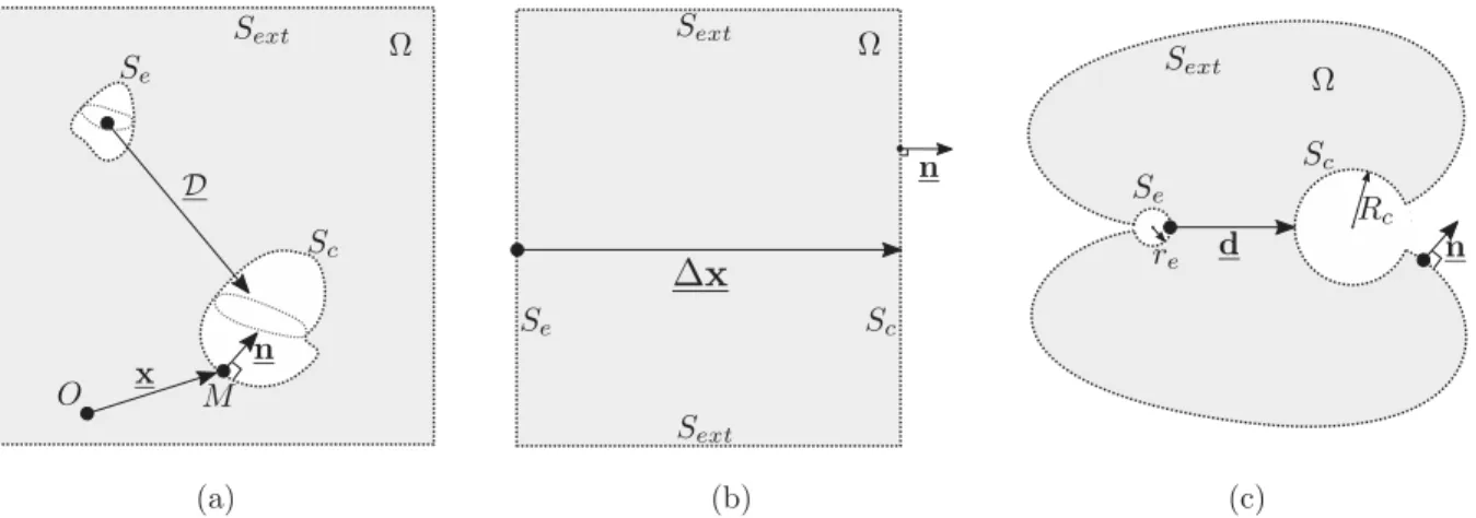
Here, we derive a simple, general formulation of the force-current relationship that we have not found elsewhere. Let us first write the general expression of the net EHD force in the configuration illustrated in Fig.1(a),
FEHD =
Z
Ä
ρE dv. (5)
Using the equality ∇ · (x ⊗ ρE) = ∇ · (ρE)x + ρE · ∇⊗x = ∇ · (ρE)x + ρE, if µ is spatially
homogeneous (constant) the local current density conservation law (2) in (5) leads to FEHD= Z Ä ∇ · (x ⊗ ρE)dv = Z ∂Ä x(ρE·n)ds, (6)
with n the outward normal and ∂Ä = Se ∪ Sc∪ Sext the boundary of Ä. Again, we were not able
to find this surface integral expression of the EHD force elsewhere. Now, considering again that the ion mobility µ is spatially homogeneous from (4), the following expression is obtained for the
(a) (b) (c)
FIG. 1. Schematic diagrams of (a) 3D general case, (b) 1D planar case, and (c) 2D wire/cylinder case. current/mobility ratio: I µ = Z Sc (ρE·n)ds. (7)
Comparing (6) and (7) thus leads to the direct relation FEHD = DI /µ, where D is an integrated
characteristic distance between the emitting and collecting electrodes. Three points can be highlighted from expression (6). First, the net thrust is independent of the choice of coordinate origin. Changing the origin from O to O′, with x = OM, does not affect (6) since
Z ∂Ä OM(ρE·n)ds = Z ∂Ä (OO′+ O′M)(ρE·n)ds = OO′ Z ∂Ä (ρE·n)ds + Z ∂Ä O′M(ρE·n)ds. Since OO′is constant and becauseR
∂Ä(ρE·n)ds = 0, we finally obtain
Z ∂Ä OM(ρE·n)ds = Z ∂Ä O′M(ρE·n)ds.
Second, the contribution of Sextis not obvious to determine theoretically. This issue can be tackled
by choosing borders parallel to the electric field lines E · n = 0. In this case, Sext defines a current
tube starting in Se and ending at Sc and encompassing the whole domain. In practice the current
density is distributed mainly in the interelectrode space: if Sext is far enough from the electrodes its
contribution can be neglected.
Third, (6) can be used to explain the robustness of the 1D result (3). For two parallel plates [as depicted in Fig. 1(b)] defined by Se = {x|x =0} and Sc = {x|x = 1x}, the derivation is
straightforward. The integral on Se is zero since x = 0, so the net force is simply
FEHD =1x
Z
Sc
ρE · nds = 1xI
µ, (8)
with I the net current and 1x = (1x,0,0). For the parallel wire-to-cylinder case illustrated in Fig. 1(c), with an emitter wire centered at x = 0 and with d the face-to-face distance between the emitting and collecting electrodes, the net force results from three contributions:
FEHD = − Z Se ren(ρE · n)ds | {z } Fe + Z Sc (re+d + Rc)ex(ρE · n)ds | {z } Fd + Z Sc Rcn(ρE · n)ds. | {z } Fc
The norm of each term can be estimated as kFek 6reµI, kFdk =(re +d + Rc)µI, and kFck 6RcµI,
respectively. In experimental EHD devices the hierarchy of scale re ≪Rc ≪dfinally leads to
FEHD ≈(re+d + Rc) I µ ≈Fd+O µ re d, Rc d ¶ . (9)
In practice, the approximation re ≪d is well verified in most ionic wind devices since the corona
discharge occurs near sharp points of electrodes. However, the collector(s) can be quite large. The current density is not uniformly distributed around the collector; it is concentrated on the surface region that faces the emitter, following Warburg’s law or similar.
Finally, we would like to provide some quantitative arguments for neglecting the corona discharge contribution to the EHD force. As is known from many studies (e.g., [20]), unipolar charges are created inside the corona discharge, reaching their maximum concentration at the interface between the corona discharge and the drift region. Furthermore, since the unipolar charge flux is balanced from the drift region, the conserved emitted current in the drift region results from unipolar charge flux at the corona dicharge/drift region interface (up to a very small electron flux associated with secondary photoemission; cf. [19] for more details). It is then possible to provide an upper bound the EHD force, FCD
EHD, associated with the corona discharge region, hereby denoted ÄCD, by using
(5): FCD EHD = R ÄCDρE dv < R ÄCDenE dv < re R
∂ÄCD≡SeenE ds. Since the unipolar charge flux from
the dc corona equals the total current divided by mobility, i.e,R∂Ä
CD≡SeenEds = I /µ, we find that
FCDEHD < reI /µso that, from (9), FCDEHD ≪FEHD, since re ≪d.
2. Principle of PIV reconstruction
Here, various approaches based on the fluid momentum equation are discussed to estimate the instantaneous spatial distribution of the volumetric force and net averaged momentum transfer. In an example given in a previous work [9], the force field around a dielectric-barrier discharge (DBD) plasma actuator was derived from the space and time derivatives of the velocity field:
ρf ∂U ∂t +ρf(U · ∇)U − ∇ · τ | {z } experimentally estimated = −∇P + fEHD | {z } unknown force , (10)
where U = (U,V ,W ) is the velocity vector, P the scalar pressure field, τ = µf(∇U + ∇TU) the
deviatoric stress tensor with µf =1.8 × 10⁻⁵ Pa s the dynamic viscosity, and fEHD the unknown
volumetric electrohydrodynamic force. This method, referred to as the derivative method throughout this paper, gives insights into the force distribution and its evolution with time. It also enables the computation of the net averaged force by integrating in space and time. In unsteady periodic flows, however, this necessitates a phase-locked PIV setup in order to compute phase averaged velocity fields, as differentiating raw instantaneous velocity fields provides inaccurate results. Another method to determine the force applied to a given fluid volume Ä would be to integrate the momentum flux through the surface ∂Ä, as in the next paragraph. This method, referred to as the integral method, does not provide a priori spatial information. For a steady EHD flow, the momentum balance is written Z ∂Ä (ρfU)U · n ds − Z ∂Ä τn ds = Z ∂Ä P n ds + Z Ä fEHDdv. (11)
Assuming uniform pressure and considering only the horizontal x component, the integral formulation reduces to the classical result
ρf
Z ¡
Uoutlet2 −Uinlet2 ¢dy = Fx, (12)
with Fxthe x component of the resultant force applied to the air volume between the inlet and outlet.
This simplified version of the integral momentum equation has been applied to an EHD thruster [14]
MONROLIN, PRAUD, AND PLOURABOUÉ
with mitigated success: the thrust computed with Uoutlet was overestimated by 70% when compared
to the reference measurements performed with a digital scale. The author explains that the knowledge of Uinlet and a better positioning of the outlet should improve the measurement.
The integral method can be used more directly and effectively with particle image velocimetry, for example. PIV has already been applied to a pulsed DBD plasma actuator [9,21,22]. However, in [21] the integral method seems to systematically underestimate the net force applied to the control volume, a weakness that does not occur with the time averaged derivative method. This indicates that temporal information is required to recover the net thrust precisely.
3. An approach for averaged velocity fields.
In a dc corona actuator, despite the steady actuation, strong velocity fluctuations can occur in the wake of the collecting electrode. Further details are given in Sec.III B. Since their occurrence can be chaotic, it is hard to synchronize any measurement device on them. In the following, we formulate an integral method that takes unsteady effects into account without requiring a time-resolved or a phase-locked PIV setup. Following the classic Reynolds decomposition, the velocity and pressure are split into a time averaged part ¯U and a time dependent one u′(t) with U(t) = ¯U + u′(t) and P (t) =
¯
P + p′(t). Using this decomposition, u′ =p′ =0 by definition. Decomposing11into average and
fluctuation finally leads to Z ∂Ä (ρfU)U · nds + Z ∂Ä ρf ¡ u′⊗u′¢nds − Z ∂Ä τ nds = Z ∂Ä P nds + Z Ä fEHDdv. (13)
The local averaged formulation can be written ρfU · ∇U + ρf∇ ·
¡
u′⊗u′¢−µ
f1U = −∇P + fEHD, (14)
bringing to the fore the usual Reynolds tensor [u′⊗u′]
ij =u′iu′j. In the present case, the flow is not,
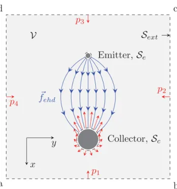
of course, truly turbulent, but velocity fluctuations are comparable with the mean flow velocity. In the following, we focus on the vertical projection of the momentum equation. The x projection of the left-hand side based on Fig.2becomes
Z ab ¯ U2+u′2dy + Z bc ¯ U ¯V + u′v′dx − Z cd U2+u′2dy − Z da ¯ U ¯V + u′v′dy = 1 ρf (−FD+FEHD). (15) In this expression, it is assumed that the viscous shear stress is negligible on abcd and that the pressure is uniform on abcd. FEHD is the net force exerted on the air due to the ion drift. FD is
the aerodynamic drag, resulting from viscous friction and non-uniform pressure distribution on the electrodes—mainly on the collector, which is a hundred times larger than the emitter. The net thrust, T, applied to the electrodes, which can be measured with a digital scale, is the opposite of the forces applied to the air:
T = −FEHD+FD. (16)
With the chosen axis convention, the EHD force applied to the air is positive (downward), which implies that the thrust on the electrodes is negative (upward). For the sake of clarity, we plot the absolute value of the thrust in all figures.
B. Experimental configuration
1. General settings
The net thrust measurements were performed with a digital scale. This first setup has been extensively used in previous publications [14,15,23,24] and was used as a reference here. A frame made of polytetrafluoroethylene (PTFE) supported electrodes of length L = 39 cm, a thin tungsten wire of diameter r = 50 µm (emitter), and one or more steel cylinders with diameter R = 1 cm [collector(s)]. The frame was hung 50 cm below the digital scale (Mettler Toledo® ME3002 0.01g).
V Sext ~ fehd a b c d p1 p2 p3 p4 x y Emitter, Se Collector, Sc
FIG. 2. Schematic of the control volume Ä and its contour ∂Ä = Se∪Sc∪Sext. The blue streamlines
represent the ion paths, hence EHD force. The red arrows represent pressure and viscous forces applied to the air by the collector.
The distance d (face-to-face) between the emitter and the collector(s) was varied between 3 and 6 cm, while the spacing s between the centers of the collectors was set from 0 (s = 0 cm corresponds to a single collector) to 10 cm. The mean current was measured by the power supply, with an accuracy of ±2.5 µA. The same frame was considered for PIV velocity measurements. In this second setup, the electrodes were placed in the middle of a cubic wooden box of edge 1 m; see Fig.3. The emitter and the collector were positioned approximately 40 cm away from the walls. Two glass windows allowed optical access to the inside of the box. The light sheet was generated with two 130 mJ lasers (Quantel CFR 200, 532 nm). The time lapse between two laser shots was adjusted so that the maximum displacement of the particle remained less than 10 pixels on the camera sensor (SensiCam PCO
1280 × 1024). Images were processed with the laboratory softwareCPIV2.2: three-pass algorithm, final interrogation windows of 16 pixels, and logarithmic subpixel interpolation, with a 50% overlap. A universal outliers detection algorithm [25] allowed for spurious vector detection.
2. Effect of seeding
Measuring velocity in electrohydrodynamic flows is more difficult than in usual aerodynamic or hydrodynamic flows. Standard techniques, such as hot wire anemometry, are inadvisable in particular between the emitter and the collector, as the probe may not withstand or may perturb the high electric field. In the present study, the optical, nonintrusive PIV measurement technique was employed to quantitatively investigate the ionic wind. This method has already been successfully used for EHD flows [26–29]. PIV requires the introduction of tracer particles into the fluid which are assumed to follow the fluid’s motion. Tracer particles must satisfy two requirements. First, they should behave as passive tracers, so their drift velocity with respect to the ionic wind must be negligible. Second, tracer particles should neither alter the electric field distribution nor influence the charge concentration. Incense smoke tracer particles were chosen as they are recognized in the literature as being among the ideal and recommendable tracers for PIV measurements in EHD gaseous flow [30,31]. Incense smoke particles have a typical density ρp =1100 kg m−3 and a typical diameter dp≈1 µm. The
latter was estimated by microscopy and its value is in agreement with previous observations [30]. The ability of particles to follow the flow is quantified by the Stokes number St = τp/τf, which compares
the particle relaxation time scale, τp =dp2ρp/18µf, with the characteristic time of the carrier fluid,
τf. For incense smoke particles in air (µf =1.85 kg m−1s−1) a characteristic time of the flow based
upon the typical measured mean velocity of the ionic wind (U0 ≈1 m s−1), and the diameter of the
collector, 2Rc =0.01 m, we estimated a Stokes number St ≈ 3 × 10⁻⁴, a value much lower than
unity. The particle settling velocity, given by d2
p1ρg/18µf, where g is the gravitational acceleration
and 1ρ the density difference between the fluid and the tracers, was close to 3 × 10⁻⁵m s−1which is
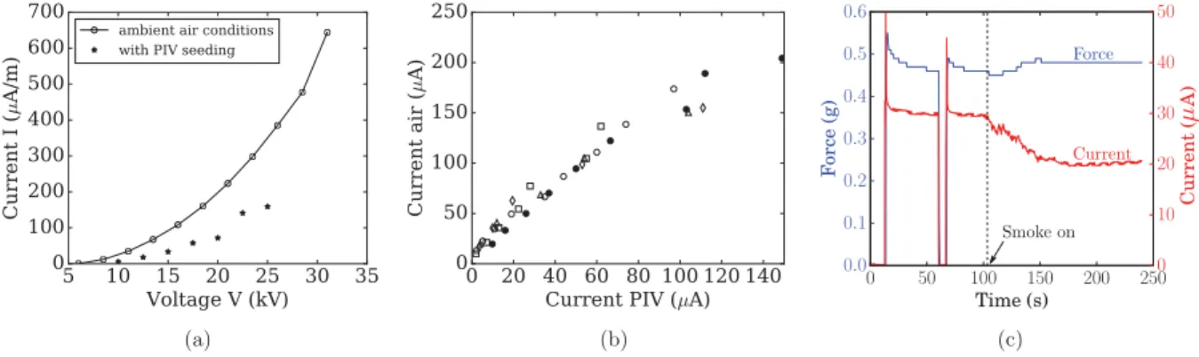
much lower than the typical measured velocity of the fluid. We can therefore consider that the tracers followed the fluid motion passively. The question regarding how PIV tracer particles might modify the ionic wind, by locally influencing the charge concentration, has been investigated by Hamdi et al. [30]. They show that the effect of incense smoke particles on the ionic wind characteristics is weak, as is the effect of an electric field on the particles. This statement is supported by our measurements which show excellent agreement between the thrust computed with PIV and the thrusts directly measured by a digital scale (see Sec.III C). These observations confirm the good accuracy of the PIV measurement and indicate that air flow and the local electrohydrodynamic force in air were only weakly affected by the smoke. The influence of incense smoke on the electrical characteristics of the discharge was also investigated. Figures 4(a) and4(b) reveal that current-voltage curves were
FIG. 4. (a) Typical current-voltage characteristic curves obtained with and without incense smoke; d = 4 cm, s = 0 cm. (b) Measured intensity in ambient air versus measured intensity with incense smoke for various cases. (c) Force (digital scale) and current versus time (d = 4 cm, s = 0 cm): voltage is set to 15 kV at t = 13 s, switched off at t = 60 s, then on again at t = 104 s with injection of smoke.
modified by incense smoke, with a decrease by a factor of around 2 in the measured intensity, a ratio which can depend on voltage. Considering (8), this decrease can be attributed to a decrease of the electrical mobility due the incense particles, which modifies the air characteristics in the experimental box (cf. Fig. 3). Remarkably, Fig. 4(c) also shows that the resulting net EHD force (in blue) was weakly affected by a 50% change in the current. This observation was robustly reproduced in all experiments conducted when varying the incense smoke concentration. This result can be understood from the theoretical prediction (9) that the net EHD force depends only on the intensity to mobility ratio, so any intensity variations concomitant with a similar mobility change (as investigated further in Sec.III C 2) result in the same EHD force.
III. RESULTS AND DISCUSSION A. PIV field
We first discuss the physics of the observed ionic wind. In this section we mainly discuss the time-averaged flow field, leaving the discussion of the flow nonstationarity to Sec.III B. The streamlines are computed from the time-average PIV velocity field in the plane orthogonal to the emitter axis. They are displayed below in Figs.5,7, and8.
1. Effect of voltage
When the emitter voltage was increased from 10 to 25 kV, a strong effect was observed on the resulting velocity, increasing its intensity by a factor of almost 5. This increase of ionic wind production took place with subtle changes in the flow field topology. For every electric potential, the air converged downstream of the emitter (the upper black spot), where a longitudinal gradient of velocity caused the air to accelerate. Since the flow field was mainly two-dimensional, providing the very small Mach number associated with this flow, incompressibility combined with longitudinal acceleration was responsible for the convergent structure of the flow field seen downstream of the emitter. At the same time, clear recirculating eddies were also visible downstream of the collector, at a distance of a few diameters from it. The intensity of these eddies also increased with the applied voltage. Following [32], we evaluated the downstream stream function ψ(x,y) = Ry
0 Ux(x,y′)dy′by
transversely integrating the longitudinal velocity field, so as to be able to clearly identify the edges of the eddies at the separation line ψ = 0. Using this separation line, we evaluated the longitudinal length of the eddies as the distance from the cylinder center to the rear stagnation point. Figure 6 compares this length with the formation length evaluated for the classical cylinder wake [33,34].
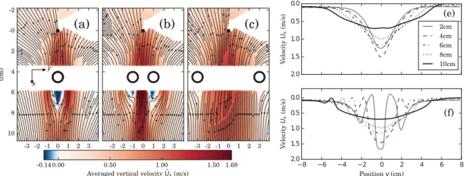
FIG. 5. (a)–(d) Vertical averaged velocity field ¯Ux and streamlines for V = 10,15,20,25 kV. Distance d =
4 cm, spacing s = 0 cm. (e) Velocity profiles 1 cm upstream of the collector and (f) maximum velocity 1 cm upstream of the collector (x = 3 cm).
FIG. 6. Eddy length versus Reynolds number, monocollector configuration, Rc=5 mm.
At moderate Reynolds number, the eddies appear longer than their classical counterparts, but, since their size decreases as the ionic wind velocity increases, this difference shrinks at higher Reynolds number.
2. Effect of distance
We now discuss the effect of the emitter/collector distance. Previous contributions (see [24] and references therein for more details) have shown that the electrode distance linearly affects the net EHD thrust, which is also proportional to the total current intensity. For a given applied electrical potential V , the local applied electric field scales as E ∼ V /d, thus decreasing with d. Figure 7 represents the velocity field measured for various distances d, but for a constant applied electric field defined by E = V /d. The longitudinal velocities are quite comparable in all panels of Fig.7, for any emitter/collector distance d. The subset Figs. 7(e)and 7(f)shows that the resulting transversal velocity profile varies only slightly as the distance between electrodes changes, for a fixed applied electric field. This can be understood from the fact that the expected ionic wind scales with the size d of the drift volume, Ud ∼p2dρE/ρf, while the Coulomb forcing term is inversely proportional to
d. Briefly, the electrostatic Poisson equation ∇2φ = −ρ/εindicates that the charge density scales as
V /d2where V is the characteristic potential difference and d the characteristic length of the problem.
FIG. 7. (a)–(d) Vertical averaged velocity field ¯Ux and streamlines for distance of d = 3, 4, 5, and 6 cm
respectively. (e) and (f) Vertical velocity profile 1 cm upstream and downstream, respectively, of the collector surface. Spacing s = 2 cm, electric field V /d = 5 kV/cm.
FIG. 8. (a)–(c)Vertical averaged velocity field ¯Ux and streamlines for various collector spacing. (e) and
(f) transversal velocity profile 1cm upstream and downstream from the collector surface. Distance d = 4 cm, voltage v = 20 kV.
Now keeping the ratio V /d constant will automatically result in ρ ∝ 1/d. Reinjecting this scaling into the momentum equation of the fluid ρf(U · ∇)U = ρE leads to ρfUd2∝ E ≈ V /d.
3. Effect of spacing
We now consider the effect of varying the spacing of collecting electrodes while keeping the applied voltage constant. Figure 8clearly shows that when the collecting electrodes are six diameters apart, the recirculating downward eddies are almost suppressed compared to the situation observed with a single collector, for which, as already mentioned in Sec. III A 1, the recirculating eddies spread over several collector diameter downstream. As a result, the longitudinal velocity field is much more transversely uniform, but less intense, in Fig. 8(c) than in Fig. 8(b). It can then be foreseen that the electrode separation will produce two opposite effects on the ionic wind. On the one hand, for small separation, it accelerates the flow downstream, with a strong transverse gradient coming from shear layers nearby collectors and significant downstream wake interactions. On the other hand, for large separation, the resulting ionic wind is much more transversely uniform, with a much smaller influence of shear layers near the collectors as well as downstream wakes but, since the local Coulomb forcing is less intense, the resulting ionic wind weakens. These velocity fields are thus clearly show that there should be an optimal separation for maximum momentum transfer into the fluid. This is then fully consistent with previously reported results (see [24] and references therein) showing an optimal thrust-to-power ratio for intermediate values of the collector separation.
B. Wake and its fluctuations
Observation of the instantaneous velocity field downstream of the collecting electrode revealed an unsteady wake associated with strong time-dependent velocity fluctuations. A spectral analysis of these velocity fluctuations in the wake of the collector was performed from the signal analysis of a hot wire probe, e(t), located 5 cm downstream of the collector. Since the probe might be sensitive to the electric field and discharge current, no precise quantitative measurement of the velocity was carried out. However, the response time was small enough for a relevant spectral analysis to be performed and temporal properties of velocity fluctuations to be highlighted. The probe-to-electrodes distance is sufficiently large to ensure that the modification of the electric field between the electrodes was negligible. The signal was recorded for 60 seconds at a frequency of 1 kHz.
The power spectral density of signal fluctuations exhibited a dominant frequency, f , which was related to a vortex shedding instability mechanism [24]. The Strouhal number was defined as Sr = 2f Rc/U0, with U0 the maximum x velocity 1 cm upstream of collector. The variation of the Strouhal
FIG. 9. Strouhal number of the velocity fluctuations in the wake of the collector versus the Reynolds number for two different distances.
number versus Reynolds number, Re = U02Rc/ν, is illustrated in Fig. 9. It is very similar to that
observed in the classical cylinder wake [35,36]. Sr first increases at low Reynolds number (Re < 700) to reach a nearly constant value of 0.3 at larger Reynolds number (Re ∼ 1000). This is slightly larger than its classical counterpart (Sr ∼ 0.2)[35]. Although the upstream velocity profile is not uniform, the experiment highlights an unsteady wake exhibiting temporal properties similar to those of the canonical cylinder wake.
C. PIV thrust computation and comparison
1. Force field deduced by the derivative method
The distribution of the volumetric force in the wire-to-cylinder coronal wind can be strongly affected by the electrode position. First, the position of the collecting electrodes affects the electric field strength at the emitter, as well as the injected charge density. Second, it also changes the ion path and consequently the size of the accelerated area. Third, the airflow is directly affected when the collectors are next to the axis of the ionic wind generator; see Sec. III A 3. Because of this three way coupling, it is hard to predict the best positions of the collecting electrodes in terms of effective momentum transfer. In the following, we reconstruct the force field from the measured velocity field. The left-hand side of (14) gives the superposition of pressure gradient ∇P and the volumetric electrohydrodynamic force fEHD. Both terms rely on a similar physical mechanism, neutral-neutral
interactions for ∇P versus ion-neutral molecular interactions for fEHD, the distinction between them
being purely theoretical. Experimentally it is not possible to distinguish them, even though ∇P is often neglected [9]. First-order and second-order derivatives are estimated with a second-order centered finite difference scheme. The air density is assumed constant and equal to 1.2 kg/m3.
The computed force field is plotted in Fig. 10. In all configurations, the force field is mainly directed along x, following the ion drift direction from the emitter to the collector. For small spacing values [cases (a) and (b)], the stagnation point on the collector generates a vertical pressure gradient that balances, and even dominates the EHD forces in the vicinity of the collector. The intensity of the force field and the size of the drift volume both increase when two collectors are used at moderate spacing values [cases (b), (c), and (d)]. For a spacing/distance ratio higher than 1, the drift volume continues to widen but also weakens. This is simply caused by a decrease of the electric field, due to the larger effective distance between emitter and collector. The best positioning of the electrodes is
FIG. 10. (a)–(f) Volumetric force reconstructed from PIV measurement (arrows), and vertical component of the force Fx(colors). Voltage V = 20 kV, distance d = 5 cm, spacing s = 0,2,4,6,8 cm.
then a tradeoff between increased charge injection, when the collectors are next to the thruster axis, and aerodynamic efficiency, which requires electrodes far from the axis.
The volumetric force, i.e., the electric current density, does not spread far from the electrodes. Visually, the typical width of the drift volume is similar to the spacing distance, which remains smaller than the camera field of view ∼16 cm. Hence, the hypothesis that the ion flow on Sext is
negligible (Sec.II A 1) is experimentally verified.
2. Net momentum by the integral method
The net force applied to the fluid could be retrieved by integrating the force field computed by the derivative method over the whole domain. However, in the present case, integration was not possible because some parts of the velocity field were missing: they were hidden by the frame supporting the electrodes. In the following, we use the integral method defined in (15). To do this, we need the velocity profile all around the domain. Still, a small part of the information on borders bc, cd, and da (cf. Fig.2sketch) is missing because of the frame. This does not significantly affect the results because the contribution of borders bc and da represents only 1% of the total net integral, whereas border cd contributes less than 15%, with only one quarter of the cd velocity profile on the right side missing. More than 85% of the net integral results from the velocity profile on border ab, which is fully available. In the following, we make the assumption that the pressure is homogeneous on the integration contour.
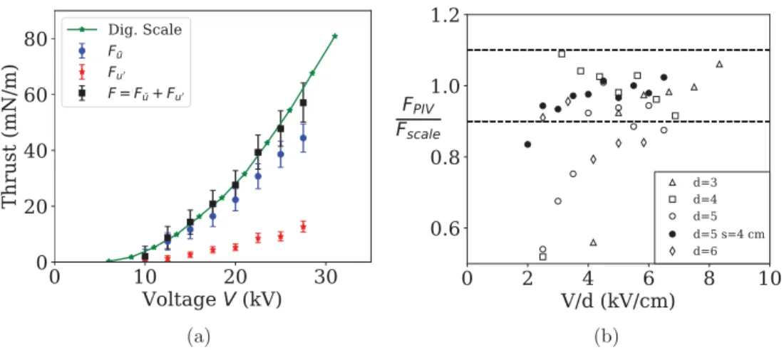
The results of configuration (d = 5 cm, s = 0 cm) are presented in Fig. 11(a). The contribu-tion of the averaged velocity field F¯u =Rabcd(ρ ¯U) ¯U · n ds · ex closely follows the digital scale
measurements for voltages lower than 20 kV. However for higher voltages the thrust is slightly underestimated, which is consistent with previous measurements made on plasma actuators [21]. This effect can be corrected by taking account of the contribution of the velocity fluctuations Fu′ =
R
FIG. 11. (a) Integral method compared to the digital scale measurement. Geometry: s = 0 cm, d = 4 cm. (b) Comparison scale/PIV for various geometries and voltages, with distinction between monocollector and bicollector cases. Dashed lines represent ±10% error range.
scale measurements. Figure 11(b)displays the thrust computed with PIV versus that measured by the digital scale for the configurations given in TableI.
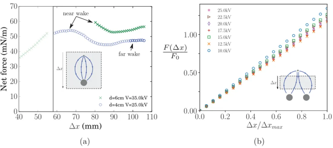
Figure11(b)clearly confirms the good accuracy of the PIV integral method. It is interesting to note that, for the largest electrode gaps (d = 5 cm and d = 6 cm), the PIV thrust is slightly underestimated. This can be explained by the integration contour being limited by the camera field of view, so that the border ab (see Fig.2sketch) eventually falls in the depression of the collector wake, thus breaking the assumption of homogeneous pressure. The minimum distance necessary between border ab and the collector to avoid the pressure gradient depends on the size of the wake eddies. The pressure effect in the “near wake region” is clearly perceptible when the size of the integration frame changes [Fig. 12(a)]. The near wake region grows as the ionic wind decreases, which explains why most low voltage cases show lower thrust than the digital scale. This could be corrected by increasing the camera field in the x direction. With spaced electrodes (case d = 5 cm s = 4 cm), the wake is much weaker (see Fig.8) and the associated pressure gradient did not affect our measurement.
One distinctive feature, occurring when the size of the rectangular integration frame is varied, is the possibility to test relation (8) which provides the slope of the momentum versus 1x in the drift region for a given electrode arrangement. The collapse of the reduced curves on Fig. 12(b) shows that this slope is proportional to the current-to-mobility ratio. A typical ion mobility value of 1.8 cm2V−1s−1 [37] was used to reduce the force in that case. Conversely, current measurements
combined with the momentum growth could be used to estimate the ion mobility. D. Energy dissipation
The proportion of electric power imparted to the fluid as kinetic energy defines the mechanical efficiency η = Pflow/Pelec. On the one hand Eq. (6) indicates that the net momentum transfer per
unit power scales as the gap distance between the electrodes whatever the electric field shape: FEHD/Pelec≈ D/µV. On the other hand the mechanical power imparted scales as the scalar
product between fluid velocity and Coulomb forcing [38,39]. The theoretical explanation is quite straightforward, but remains poorly quantified experimentally. In the following the variation of
TABLE I. Configurations associated with Fig.11(b).
d(cm) 3 4 5 5 6
s(cm) 0 0 0 4 0
FIG. 12. (a) Integrated force F = Fu+Fu′ versus integration frame length when border ab is in the
collector wake. (b) Nondimensional integrated force, with Fo =I × 1xmax/µ0and µ0 =1.8 cm2V−1s−1, vs
nondimensional integration frame length; d = 5 cm, s = 4 cm. The integration frame starts below the emitter at x0 =1 cm to avoid hidden areas.
efficiency with geometry is investigated. First of all, let us write the kinetic energy integral balance Z ∂Ä ρkUk 2 2 U · n ds | {z } Pflow = Z Ä fEHD·U dv | {z } PEHD + Z ∂Ä P U · n ds | {z } Pp + Z ∂Ä U ·(τ n)ds | {z } Pvis . (17)
Pflow is the total kinetic power gained by the airflow and PEHD, Pp, and Pvis are the kinetic power
source/sink due to electrohydrodynamic forces, pressure, and viscous dissipation respectively. Note that Pp =0 since U = 0 on Se and Sc and Pext
R
SextU · nds =0 because of incompressibility. To
account for the unsteady wake, we apply the Reynolds decomposition [U]i =Ui+u′i to Eq. (17).
Introducing the mean flow specific kinetic energy K = UiUi/2 and the turbulent specific kinetic
energy k = u′ iu
′
i/2, the momentum balance reads
Z ∂Ä ρK ¯Uj njds | {z } Pmean + Z ∂Ä ¡ k ¯Uj +12u′iu′iu′j + ¯Uiu′iu′j ¢ njds | {z } Pturb =PEHD+Pvis. (18)
The evaluation of Pflow = Pmean + Pturb from PIV data is made possible by neglecting the third component of the velocity. Note that this assumption holds only for a strictly two-dimensional flow and not, properly speaking, for a 3D turbulent flow. Figure 13 shows that the electric to kinetic energy conversion efficiency depends strongly on the spacing between the electrodes. For θ < 20◦, a
non-negligible part of the power imparted is dissipated in the shear layers and eddies induced by the collector(s). Then for θ ≈ 30◦the efficiency reaches a maximum before decreasing with increasing
angle θ. This decrease relies on the scalar product inside PEHD, so that the efficiency should scale as
cos(θ). The contribution of velocity fluctuations Pturb/Pelec to the net kinetic power is approximately
constant. The proportion of turbulent to mean kinetic power typically varies between 16% for θ = 30◦
and 50% in the monocollector case.
E. Effective mobility
In this section, the effect of incense smoke on the ionic wind generator is analyzed in terms of effective mobility. We first review the parameters influencing the mobility of positive air ions and the associated experiments. Then, we introduce a new method for quantifying the effective mobility inside the corona drift region.
1. Mobility of positive air ions
The positive ion mobility in air is subject to variations depending on pressure, temperature, humidity and lifetime, and even electric field strength when E/N & 40 Td (E > 106V/m in standard
atmospheric conditions). This last dependence, illustrated by Fig. 14(b), is not expected to play a major role in the drift region where E ∼ V /d < 8 × 10⁵V/m. There are numerous measurements of
the mobility of corona ions [14,37,40,41], with values ranging from 1.1 to 3 cm2V−1s−1depending
on the method used. Most of the time, the mobility is measured near the inception voltage, by linearizing the I -V characteristic. This method, discussed and enhanced by Stearn [37], provides information only at the inception voltage and gives values near 1.8 cm2V−1s−1. When calculating
the ionic mobility from the thrust/current ratio at various voltages in a corona thruster, Moreau [14] found 3 cm2V−1s−1. This method, as explained by Moreau and Monrolin [15,24], is however biased
by the aerodynamic drag on the collector. Besides mass spectrometry/differential mass analyser experiments [40,41] give a mobility between 1.2 and 1.4 cm2V−1s−1[results from [40] transposed
to 293 K with Eq. (2) given in the reference]. This method shows that ion mobility decreases for ages greater than 10 ms. However, in typical corona devices with d < 6 cm, E > 1 kV/cm, and µ > 1 cm2V−1s−1, the time of flight d/µE between the electrodes is less than 6 ms. Hence, the
previous considerations concerning ion aging are not relevant to our experimental conditions. Calculations based on the ion clustering kinetics [42] with the most common positive air ions, H3O+(H2O)n, O+2(H2O)n, NO+(H2O)n, and NO+2(H2O)n, show that clustering for n = 1, . . . ,7
occurs in less than 1 ms. Figure 14(b), retrieved from the LXcat data project [43], typically shows that cluster ions mobility decreases as the number of aggregated water molecules increases. Other contaminant vapors (ethanol, acetone, or ammonia) can also aggregate to ions [44], and this could be the case with incense burning products. In the Appendix we quantify the influence of incense smoke on the effective mobility.
IV. CONCLUSION
In this paper a surface formulation of the EHD force in dc-corona discharge is developed and applied to the wire-to-cylinder configuration so as to derive simple theoretical expressions for its dependence on the current-to-mobility ratio, and a geometrically dependent length. By combining PIV measurements with force-field reconstruction, we show that velocity fluctuation effects considered in momentum transfer have non-negligible effects on the EHD force calculation.
FIG. 13. Kinetic to electric power ratio versus collector spacing angle tan θ = s/(2d). Empty symbols combine both stationary and fluctuating contributions while filled symbols are the contribution of fluctuating contributions only.
FIG. 14. (a) Effective mobility µeff versus reference electric field V /d. (b) Measured mobility of positive
core ions in air or pure nitrogen at 300 K, 1 bar from Vielhand [45], retrieved from the LXcat data project. We identify that these unsteady effects are associated with downstream vortex shedding at collectors, for which we measure the corresponding constant Strouhal number (close to 0.3). We also analyze the eddies associated with the downstream wake and compare them with classical ones. Looking deeper into the physical mechanisms associated with maximum EHD lift force configuration in the separated collector pair configuration, we visualize and quantify the disappearance of the eddies, which explains the suppression of wake shedding and results in an increase of the lift force. Finally, the efficiency variations with geometry are fully consistent with the picture emerging from the previous momentum transfer analysis. The energy transfer is found to be maximum for a suitably separated collector pair, and the effect of the fluctuation is indeed weakened when the separation suppresses the wake shedding.
ACKNOWLEDGMENTS
This work was supported by the CNES (research contract 5100015475) and the French Occitanie region. We thank P. Elyakime for theCPIVsoftware support and S. Cazin, M. Marchal, and I. Loukili for their technical assistance. The authors also acknowledge L. Pitchford and JP. Boeuf for useful discussions on ionic mobility.
APPENDIX
A method for estimating the effective mobility directly inside the corona drift region is proposed, by measuring the ionic wind momentum growth rate. First, the fluid momentum equation for the control surface described in Fig.12(b), inside the drift region, is
Z
∂Ä(1x)
(ρfU)U · n ds = FEHD(1x), (A1)
where 1x is the size of the integration frame sketched in Fig. 12(b). An obvious linear trend is visible, predicted by (8). We assume that pressure gradient are negligible inside the chosen control surface. From (8) giving FEHD(1x) and by differentiating Eq. (A1) along 1x, the effective mobility
reads µeff = I d d(1x) R abcd(ρfU)U · n ds . (A2)
The effective mobility µeff obtained using (A2) is presented in Fig.14(a). The measurement shows
that µeff ranges from 1 to 2.5 cm2V−1s−1and that there is a global increasing trend with increasing
applied voltage. No definitive conclusion can be drawn since the recorded growth is of the same order as the uncertainty level. The points “Low,” “Med.,” and “High” in Fig.14(a)correspond to the case (d = 5 cm, s = 0 cm, V = 20 kV) with three different seeding densities: low, medium, and high. The measured currents were respectively 56, 55, and 46 µA/m compared to 127 µA/m obtained without seeding. On the other hand, the net integrated thrust gave 23.8, 20.8, and 19.7 mN/m compared to 21.4 mN/m obtained with a digital scale without seeding. Meanwhile, the effective mobility varied from 1.8 to 1.25 cm2V−1s−1. The measured mobility increased by at least 40% when smoke
concentration decreased. It can further be shown that smoke dissipation is increased by strong ionic wind, so the increasing mobility trend could be due to a decreasing averaged smoke density at high voltages.
It is, however, undeniable that smoke concentration has little effect on the thrust while, in contrast, the current is nearly halved, even at low smoke concentration. Section II A 1 highlights that F ∼ I /µ ∼ ρEis independent of mobility, while I ∼ ρµE is proportional to it. This observation indicates that the effective mobility of the charge carriers is decreased in the presence of smoke. This is in accordance with the measured ionic mobility which was in the range 1–1.5 cm2V−1s−1while typical
mobility of corona ions lies around 1.8 cm2V−1s−1[37]. The precise explanation of why the effective
mobility drops remains unclear. As previously discussed, the ion clustering process could change in the presence of incense burning products. Since the kinetics and composition of the air ion mixture is rather complex, most studies on corona discharge consider a constant mobility. One might voice the possibility that some incense particles become charged in the drift region, thus contributing to the momentum transfer, as ions. If true, this should be detectable experimentally by particles following electric field lines rather than airflow streamlines, which is never observed. From the theoretical viewpoint, the electrodrifting velocity of the particles resulting from the balance between Coulomb force and Stokes drag is d2
pρE/18µf, and in experimental conditions it is close to 3 × 10⁻² m s−1
which is much lower than the typical measured velocity. So this effect is not relevant here.
[1] A. Fridman, A. Chirokov, and A. Gutsol, Non-thermal atmospheric pressure discharges,J. Phys. D Appl. Phys. 38,R1(R)(2005).
[2] H. A. Erikson, On the nature of the negative and positive ions in air, oxygen and nitrogen,Phys. Rev. 20,
117(1922).
[3] E. A. Christenson and P. S. Moller, Ion-neutral propulsion in atmospheric media,AIAA J. 5,1768(1967). [4] P. Durbin and L. Turyn, Analysis of the positive DC corona between coaxial cylinders, J. Appl. Phys. 20,
1490 (1987).
[5] R. Morrow, The theory of positive glow corona,J. Phys. D Appl. Phys. 30,3099(1997).
[6] H. Bondar and F. Bastien, Effect of neutral fluid velocity on direct conversion from electrical to fluid kinetic energy in an electro-fluid-dynamics (EFD) device,J. Phys. D Appl. Phys. 19,1657(2000). [7] D. B. Go, R. A. Maturana, T. S. Fisher, and S. V. Garimella, Enhancement of external forced convection
by ionic wind,Int. J. Heat Mass Tran. 51,6047(2008).
[8] D. F. Colas, A. Ferret, D. Z. Pai, D. a. Lacoste, and C. O. Laux, Ionic wind generation by a wire-cylinder-plate corona discharge in air at atmospheric pressure,J. Appl. Phys. 108,103306(2010).
[9] N. Benard, A. Debien, and E. Moreau, Time-dependent volume force produced by a non-thermal plasma actuator from experimental velocity field,J. Phys. D Appl. Phys. 46,245201(2013).
[10] D. Cagnoni, F. Agostini, T. Christen, N. Parolini, I. Stevanovic, and C. de Falco, Multiphysics simulation of corona discharge induced ionic wind,J. Appl. Phys. 114,233301(2013).
[11] C. K. Gilmore and S. R. H. Barrett, Electro-hydrodynamic thrust density using positive corona-induced ionic winds for in-atmosphere propulsion,Proc. R. Soc. London A 471,2175(2015).
[12] K. Masuyama and S. R. H. Barrett, On the performance of electrohydrodynamic propulsion, R. Soc. London Proc. Ser. A 469,20623(2013).
[13] E. Moreau and G. Touchard, Enhancing the mechanical efficiency of electric wind in corona discharges,
J. Electrostat. 66,39(2008).
[14] E. Moreau, N. Benard, J.-D. Lan-Sun-Luk, and J.-P. Chabriat, Electro-hydrodynamic force produced by a wire-to-cylinder dc corona discharge in air at atmospheric pressure,J. Phys. D Appl. Phys. 46,475204
(2013).
[15] E. Moreau, N. Benard, F. Alicalapa, and A. Douyère, Electro-hydrodynamic force produced by a corona discharge between a wire active electrode and several cylinder electrodes - Application to electric propulsion,J. Electrostat. 76,194(2015).
[16] P. Cooperman, A Theory for space charge limited currents with application to electrical precipitation,
Trans. AIEE, Part I: Commun. Electron. 79,47(1960).
[17] R. S. Sigmond, Simple approximate treatment of unipolar space-charge-dominated coronas: The Warburg law and the saturation current,J. Appl. Phys. 53,891(1982).
[18] J. R. Roth, Industrial Plasma Engineering (IOP, London, 1995), Vol. 1, Chap. 8, pp. 251–269.
[19] N. Monrolin, F. Plouraboué, and O. Praud, Revisiting the positive DC corona discharge theory: Beyond Peek’s and Townsend’s law, Plasma Phys. (to be published).
[20] Y. Zheng, B. Zhang, and J. He, Currentvoltage characteristics of dc corona discharges in air between coaxial cylinders,Phys. Plasmas 22,023501(2015).
[21] M. Kotsonis, S. Ghaemi, L. Veldhuis, and F. Scarano, Measurement of the body force field of plasma actuators,J. Phys. D 44,045204(2011).
[22] M. Kotsonis, Diagnostics for characterisation of plasma actuators,Meas. Sci. Technol. 26,092001(2015). [23] K. N. Kiousis, A. X. Moronis, and W. G. Fruh, Electro-hydrodynamic (EHD) thrust analysis in
wire-cylinder electrode arrangement,Plasma Sci. Technol. 16,363(2014).
[24] N. Monrolin, F. Plouraboué, and O. Praud, Electro-hydrodynamic thrust for in-atmosphere propulsion,
AIAA J. 55,4296(2017).
[25] J. Westerweel and F. Scarano, Universal outlier detection for PIV data,Exp. Fluids 39,1096(2005). [26] A. Santhanakrishnan, J. D. Jacob, and Y. B. Suzen, Flow control using plasma actuators and linear/annular
plasma synthetic jet actuators, in 3rd AIAA Flow Control Conference (2006), doi:10.2514/6.2006-3033. [27] M. Kotsonis and S. Ghaemi, Experimental and numerical characterization of a plasma actuator in
continuous and pulsed actuation,Sens. Actuators, A 187,84(2012).
[28] A. Debien, N. Benard, and E. Moreau, Streamer inhibition for improving force and electric wind produced by DBD actuators,J. Phys. D Appl. Phys. 45,215201(2012).
[29] E. Pescini, DS Martínez, M. G. De Giorgi, and A. Ficarella, Optimization of micro single dielectric barrier discharge plasma actuator models based on experimental velocity and body force fields,Acta Astronaut.
116,318(2015).
[30] M. Hamdi, M. Havet, O. Rouaud, and D. Tarlet, Comparison of different tracers for PIV measurements in EHD airflow,Exp. Fluids 55,1702(2014).
[31] P. Magnier, D. Hong, A. Leroy-Chesneau, J.-M. Bauchire, and J. Hureau, Control of separated flows with the ionic wind generated by a DC corona discharge,Exp. Fluids 42,815(2007).
[32] D. Lo Jacono, M. Nazarinia, and M. Brøns, Experimental vortex breakdown topology in a cylinder with a free surface,Phys. Fluids 21,111704(2009).
[33] J. H. Gerrard, The wakes of cylindrical bluff bodies at low Reynolds number,Philos. Trans. R. Soc. A 288,
351(1978).
[34] H. G. C. Woo, J. E. Cermak, and J. A. Peterka, Experiments on vortex shedding from stationary and oscillating cables in a linear shear flow, technical report, Colorado State University, Fort Collins, 1981 (unpublished).
[35] F. L. Ponta and H. Aref, Strouhal-Reynolds Number Relationship for Vortex Streets,Phys. Rev. Lett. 93,
084501(2004).
[36] A. Capone, C. Klein, F. Di Felice, and M. Miozzi, Phenomenology of a flow around a circular cylinder at sub-critical and critical Reynolds numbers,Phys. Fluids 28,074101(2016).
[37] R. G. Stearns, Ion mobility measurements in a positive corona discharge,J. Appl. Phys. 67,2789(1990). [38] C. Kim, K.-C. Noh, J. Hyun, S.-G. Lee, J. Hwang, and H. Hong, Microscopic energy conversion process
[39] O. Stuetzer, Magnetohydrodynamics and electrohydrodynamics,Phys. Fluids 5,534(1962).
[40] M. Alonso, J. Santos, E. Hontañón, and E. Ramiro, First differential mobility analysis (DMA) measure-ments of air ions produced by radioactive source and corona, Aerosol Air Qual. Res. 9, 453 (2009). [41] N. Fujioka, Y. Tsunoda, A. Sugimura, and K. Arai, Influence of Humidity on Variation of Ion Mobility
with Life Time in atmospheric Air,IEEE Trans. Power Apparat. Sys. 102,911(1983).
[42] M. L. Huertas and J. Fontan, Evolution times of tropospheric positive ions,Atmos. Environ. 9,1018(1975). [43] FLINDERS database,www.lxcat.net, retrieved on September 12, 2017.
[44] M. L. Huertas, A. M. Marty, J. Fontan, and G. Duffa, Measurement of mobility and mass of atmospheric ions,J. Aerosol. Sci. 2,145(1971).
[45] L. Viehland and C. Kirkpatrick, Relating ion/neutral reaction rate coefficients and cross-sections by accessing a database for ion transport properties,Int. J. Mass Spectrom. 149,555(1995), special issue, Honour Biography David Smith.