Morlet Wavelet transformed holograms for numerical adaptive view-based reconstruction

HAL Id: hal-01115531

https://hal.archives-ouvertes.fr/hal-01115531

Submitted on 14 Dec 2015

HAL is a multi-disciplinary open access

archive for the deposit and dissemination of

sci-entific research documents, whether they are

pub-lished or not. The documents may come from

teaching and research institutions in France or

abroad, or from public or private research centers.

L’archive ouverte pluridisciplinaire HAL, est

destinée au dépôt et à la diffusion de documents

scientifiques de niveau recherche, publiés ou non,

émanant des établissements d’enseignement et de

recherche français ou étrangers, des laboratoires

publics ou privés.

Morlet Wavelet transformed holograms for numerical

adaptive view-based reconstruction

Kartik Viswanathan, Patrick Gioia, Luce Morin

To cite this version:

Kartik Viswanathan, Patrick Gioia, Luce Morin. Morlet Wavelet transformed holograms for

numer-ical adaptive view-based reconstruction. Proc. SPIE 9216, Optics and Photonics for Information

Processing VIII, 92160G (19 September 2014), Aug 2014, San Diego, United States. �hal-01115531�

See discussions, stats, and author profiles for this publication at: http://www.researchgate.net/publication/266369125

Morlet Wavelet transformed holograms for numerical adaptive

view-based reconstruction

CONFERENCE PAPER in PROCEEDINGS OF SPIE - THE INTERNATIONAL SOCIETY FOR OPTICAL ENGINEERING · SEPTEMBER 2014 Impact Factor: 0.2 · DOI: 10.1117/12.2061588 READS 45 3 AUTHORS: Kartik Viswanathan Institut National des Sciences Appliquées de Rennes 2 PUBLICATIONS 2 CITATIONS SEE PROFILE Patrick Gioia Orange Labs 40 PUBLICATIONS 200 CITATIONS SEE PROFILE Luce Morin Institut National des Sciences Appliquées de Rennes 110 PUBLICATIONS 381 CITATIONS SEE PROFILE Available from: Kartik Viswanathan Retrieved on: 14 December 2015

Morlet Wavelet transformed holograms for numerical

adaptive view-based reconstruction

Kartik Viswanathan

a

and Patrick Gioia

a

and Luce Morin

b

a

_{Orange Labs, France;}

b

_{INSA, Rennes, France}

ABSTRACT

We provide an efficient method of using Morlet wavelets for transforming a hologram and reconstructing parts of a scene based on the position of viewer by using a sparse set of Morlet transformed coefficients. We provide a design of a Morlet wavelet and explain an efficient discretization method for the application of view-dependent representation systems. Results are provided based on the numerical reconstruction, and it is shown that view-dependent representation along with Morlet wavelets form a good starting step for compressing holographic data for next generation 3DTV applications.

Keywords: View-dependent representation, Digital Holography, Morlet wavelets, Gabor basis, Adaptive recon-struction

1. INTRODUCTION

The compression of digital holograms is one of the major challenges in the transmission of digital holographic data for next generation 3DTV applications. The sheer large amount of information cannot be sustained by current network bandwidth capabilities. The conventional methods of compression have been applied to holograms. MPEG2 compression has been used by Darakis et al. (1_{) and JPEG2000 is proposed by Xing et al. (}2_{), They}

have shown to provide significant gain but still are not sufficient enough for today’s network bandwidths. This is because conventional compression methods exploit spatial redundancies, whereas holograms present little or no spatial correlations. Moreover classical compression methods cut down high frequency information which are critical for hologram reconstruction.

We propose an alternative strategy based on the assumption that the resulting transmitted hologram is displayed for only a limited number of viewers. The principle of this type of view-based compression lies in the fact that all the data need not be present for reconstruction and only sparse sets of information are transmitted based on the location of the viewer. This method has been outlined in (3₎₍4_{). As the direction of emission}

(towards a viewer) of each hologram element is directly linked to the frequency range, a precise spectral and spatial representation of the hologram is required to achieve view-based representation.

Wavelets are a natural choice for performing both space and frequency analysis. In addition to this property, we also need to have a best possible localization in space and frequency domains, as improper localization will result in poor angular resolution of the view-based reconstruction (4_{). Among the classical wavelet families, the}

ones based on the Gabor basis functions and the derived wavelet families provide the best theoretical space-frequency localization that can be possible (5_).

There have been earlier uses of the Gabor wavelet transform for edge detections, face recognitions, MPEG-7 based applications (6_{), and also in hologram compression (}7_{). But the type of the transform was the Max-Gabor}

transform (8_{), in which the maximum value of the gabor coefficients were stored for each location and the others}

discarded. This in essence meant only storing the dominant frequency information for a localized region in an image. This approach is very intutive and is also very apt for 2D images or 3D images that contain very less

Further author information:

E-mail: kartik.viswanathan@orange.com, Telephone: +33 (0)299124994 E-mail: patrick.gioia@orange.com, Telephone: +33 (0)299124198 E-mail: luce.morin@insa-rennes.fr, Telephone: +33 (0)223238757

Figure 1. Gabor function formed by combining a Gaussian and a complex sinusoid

information. But when we talk about holographic data, no frequency information can be discarded. As all frequencies can contribute to the reconstruction of the 3D scene.

There are two main problems that arise with Gabor basis functions which are failure of the admissibility condition and unequal sizes of the sinusoids for various frequencies (5₎₍9_{). Admissibility is a mathematical}

condition that ensures reversibility. The same size of the wavelet at different scales ensures that the spatial features at all frequencies are evenly approximated, since the number of oscillations within the window function is always a constant as will be seen in the next section. In order to overcome these two issues, we propose using Morlet wavelets (10)(11) which are derived from Gabor basis functions.

The following sections discuss the design and implementation of a view-based representation system based on Morlet wavelets. Section 2 provides the basic theory of the Gabor basis function and gives the continuous form of the 2D Morlet wavelet. Section 3 shows the discretization of, the Morlet wavelet in continuous form, with respect to the application of view-based compression systems. In Section 4 we provide a step by step approach to select the parameters of the Gabor basis for a simple cube scene. In Section 5 we show the results for the cube hologram using the discrete Morlet wavelets that we designed in the previous section.

2. THE GABOR BASIS FUNCTION AND THE MORLET WAVELET

There have been earlier uses of the Gabor basis functions for edge detections, face recognitions, MPEG-7 based applications (6), and also in hologram compression (7). In this section we begin by reminding the concepts of the Gabor basis function. We derive the design of the Morlet wavelet beginning with the Gabor function in the 1D form, and then moving to the 2D form of the Morlet wavelet.

A Gabor function is formed by combining a sinusoid and a Gaussian. Figure(1) shows this for the 1D form. The Gabor function which is chosen is taken in the complex form because the best theoretical space-frequency localization is obtained in the complex form(5_{). Gabor basis in the one dimensional continuous form is defined}

as

gβ,f0(x) = K.w(βx)s(2πf0x) (1)

where,

w(x) = exp(−x2), (2)

where f0is the frequency of the sinusoid, K is the norm of the basis function and β is a function of the parameter

of the Gaussian function σ. β is given as,

β2= 1

2σ2. (4)

The full width at half maximum (FWHM) or 3dB width of the Gaussian is given as

Ws= 2

p

2 ln(2)σ (5)

Taking the Fourier transform of Equation(1), we get the spectrum G of the Gabor basis function,

Gβ,f(f ) = K.

Z ∞

−∞

w(βx). exp(j2πf0x). exp(−j2πf x)dx (6)

In order to have equal number of oscillations for all frequencies, we choose

f0= 1 √ 2π 2_{β. (7)} Hence, β = √ 2f0 π , (8) ˆ gβ,f(f ) = K. Z ∞ −∞ exp(−j2π(f − f0)x).w(βx).dx, (9) ˆ gβ,f(f ) = K βw(ˆ f − f0 β ), (10) where, ˆ w(f ) = exp(−π2f2). (11) Equation(10) shows that ˆgβ,f(f ) is centered at f0, i.e the peak is at this frequency. The half magnitude bandwidth

(HMB) will be

Wf = β =

1 √

2σ (12)

Equation(8) gives the important relation between the parameter β related to the Gaussian function, and the frequency of the sinusoid f0. Later the parameter β can be varied for centering the Gabor function on different

frequencies. As it can be observed from Equation(5) and Equation(12), the product of the Wsand Wf is always

a constant and it independent of the parameter σ. This shows the good localization property of the Gabor basis function in space and frequency domains as discussed in (4_).

To enforce the admissibility condition we introduce a term to eliminate the DC response of the filter. The elimination of the DC term is as shown in Appendix(A). Equation(13) defines the Morlet mother wavelet in 1D form.

g(x) = K. exp(−β2x2)(exp(2πjf0x) − exp(−

π2

β2f 2

0)). (13)

For deriving the 2D Morlet wavelet in the continuous 2D form, we consider the basic Gabor function equation with the parameter of the Gaussian function in the x and y directions to be β. From Equation(13) extended in 2D, we get

g(x, y) = K. exp(−β2(x2+ y2))(exp(2πj(u0x + v0y)) − exp(−

π2 β2(u 2 0+ v 2 0))), (14)

where u0 and v0 are the spatial frequencies in x and y directions respectively. K is a multiplier, which is the

L2-norm of the basis (12), and the term exp(−π_β22(u

2

0+ v02)) is introduced to eliminate the DC response of the

Similar to the 1D case we include equal number of oscillations for all frequencies, by setting

u2₀+ v2₀= π2β2 (15)

where u0 and v0 are obtained according to Equation(8) Therefore,

exp(−π 2 β2(u 2 0+ v 2 0)) = exp(− π2 β2π 2_β2_{) = exp(−π}4_{) ≈ 0 (16)}

Representing the spatial frequencies u0 and v0 into polar form

u0= F0cosθ, v0= F0sinθ, (17)

where, F02= u20+ v20.

We consider a continuous variation in the rotation parameter denoted by θ. The variation of θ in essence signifies the variation of the spatial frequencies in x and y directions of the Gabor function. The general equation of the Gabor function in 2D continuous form becomes

ψ(x, y) = g(x, y) = K. exp(−β2(x2+ y2)) exp(2π2βj(xcosθ + ysinθ)) (18)

Equation(18) is the Morlet mother wavelet in 2D form, which will be denoted as ψ(x, y) from now on. It can be used as a basis for the application in view-based representation of holograms.

In order to build the family of Morlet wavelets we introduce the scale parameter in its continuous form in 1D and then extend it to 2D form. The Morlet mother wavelet function in one dimensional form from equation(1), where β = √ 2fo π is given as follows: ψ(x) = K. exp(−2f 2 ox2 π2 ). exp(j2πfox) (19)

The Fourier transform is given according to Equation(10) and centered at fo

ˆ ψ(f ) = Kπ 4 2f2 o exp(−π 4_{(f − f} o)2 2f2 o ) (20)

We can consider Equation(19) like a mother wavelet centered at fo. The suitable translation and dilation of this

equation will give us a family of basis functions that will span the frequency plane. The parameter s controls the spatial and frequency resolution of the basis decomposition. The scaled frequencies based on parameter s will be given as:

f =fo

s (21)

The Full width at half maximum (Ws) and Half magnitude bandwidth (Wf) will be scaled as:

Ws= Wso.s π 2fo (22) Wf = Wfo s (23)

where s > 0. The generic Morlet wavelet ψs,b is given as

ψs,b(x) = K. exp(− 2f2 ox2 π2 (x − b)2 s2 ). exp(j2πfo (x − b) s ), (24)

where, s is the scaling parameter and b is the translation parameter. Each ψs,b(x) contains the local frequency

From Equation(18) we can give the 2D form of the Morlet wavelet centered at fo = pu2o+ vo2, with the parameters s and θ ψs,θ(x, y) = K. exp(− f2 o s2_π2(x 2_{+ y}2_{)) exp(2π}2fo sπj(x cos θ + y sin θ)) (25) The variation of s and θ allows for the spanning of the spatial frequencies along the x and y directions. For example, 3 rotations and 3 scales of the 2D basis function shall provide for 9 different combinations of spatial frequencies.

It can be noted the scaling parameter s, scales both the sinusoid as well as the gaussian function.

3. DISCRETIZATION OF THE MORLET WAVELET

The analysis so far is limited to the continuous domain. The theory so far presented is very close to the theory of Continuous Wavelet transforms (CWT). The Morlet Wavelet does not have a unique spanning function. Instead the spanning of the frequency domain are done at discrete frequencies as it will be explained in this section. To begin with the discretization, we need to identify the degrees of freedom that the Morlet wavelet provides. It gives us 4 degrees of freedom, namely x, y, s and θ, and these need to be suitably discretized for the application of view based representation of holograms.

We begin by the discretization of x and y. As seen in Equation(1), the Gabor function is composed of a sinusoid enveloped by a Gaussian. We begin by considering a suitable length of the Gaussian given by L. The length L is selected based on the tapering of the Gaussian function where the values can be considered to be close to 0. We then ensure that there are Nooscillations of the sinusoid with frequency f0within this Gaussian.

The length of the Gabor function hence becomes:

L = No f0

. (26)

This ensures that there are equal number of oscillations within the Gaussian irrespective of the frequency. For the discretization of the function we use the Nyquist criterion. The sampling frequency fsis selected to be twice

the frequency of the sinusoid. This gives us the actual size of the analog window function Lw that is needed for

the numerical representation of the Gabor function.

Lw= L.fs (27a)

= No f0

.2f0 (27b)

= 2No (27c)

We consider the analog window size to be equal in both the spatial directions.

The position of the viewer with respect to the field of reconstruction, gives the angle at which the diffraction reaches the observer. This is according to the Grating equation given as

θdif f = arcsin(λf ) (28)

where f represents the spatial frequency of the hologram, λ is the wavelength of light and θdif f is the angle

of diffraction. For discrete positions of the observer we can discretize the observer plane, which in turn means discretizing the scale and rotation of the Morlet wavelet.

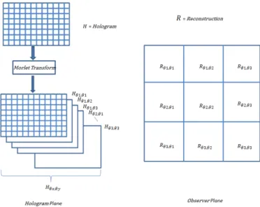
The discretization of the scale parameter is done based on the discrete positions of the viewer in the recon-struction plane. The Figure(2) illustrates this concept. The Morlet transform of the hologram H will give Hθx,θy,

the decomposition of the field in terms of spatial frequencies. The spatial frequencies have a direct relation with the angle of diffraction θx and θy given by the grating Equation(28). In Figure(2) the reconstruction plane

Figure 2. Discretization of Reconstruction plane

on the observer position, the proximity to a zone can be computed, and the relevant Hθx,θy is selected for the

reconstruction process.

Next we discretize the rotation parameter θ. We perform Nθ rotations of the sinusoid from 0 to π. The

discrete rotation parameter is denoted as r.

The discrete spatial frequencies in x and y directions fxand fy are given as

fx= fccos(Θr) l , (29a) fy= fcsin(Θr) l , (29b)

The relation between the discrete angles of diffraction θx and θy, and the discrete scale parameter l and the

discrete rotation parameter r is obtained by combining Equation(29) and Equation(28)

θx= arcsin(λ fc l cos(Θr)), (30a) θy = arcsin(λ fc l sin(Θr)), (30b) where Θ =_Nπ

θ and 0 ≤ r < Nθ and Nθ> 0 is integer.

We have in this manner discretized the 4 degrees of freedom of the Morlet wavelet Equation(25). The final discretized equation of the the Morlet wavelet is given as:

gl,r[m, n] = K. exp(− f_c2 l2_π2(m 2_{+ n}2_{)) exp(2π}2fc lπj(m cos(Θr) + n sin(Θr))) (31) where −M 2 ≤ m < M 2 and − N 2 ≤ n < N

2 and M and N are given according to Equation(27) and are integers,

l > 0 and real.

fcis selected based on the maximum frequency that is possible for the given display setup. In our experiments

it is given as:

fc=

1

P , (32)

Figure 3. The Morlet Transform

In Figure(2) it can be noted that there are 9 discrete Rθx,θy zones of reconstruction. 3 values of the rotation

discretization parameter r and 3 values of the scale discretization parameter l are sufficient to obtain the 9 different Morlet wavelet decompositions to reconstruct the hologram.

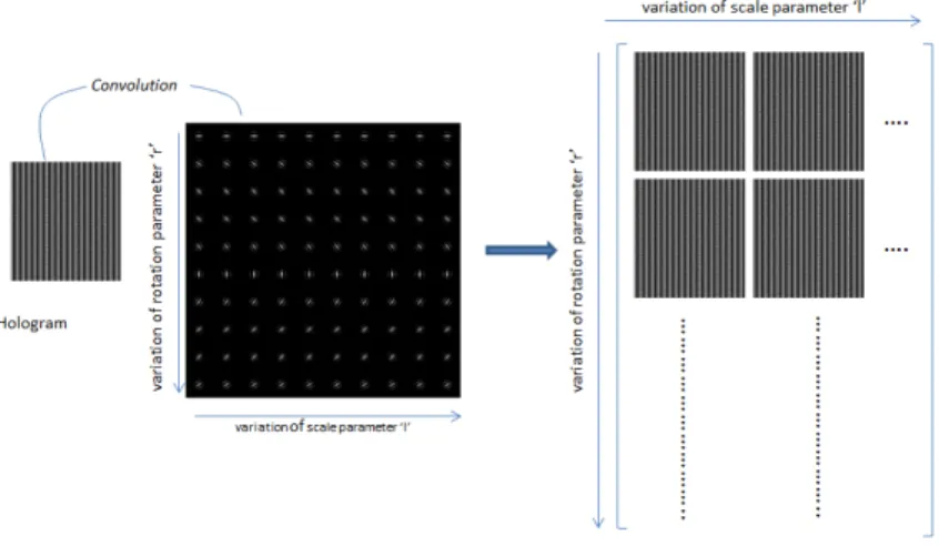
Figure(4) shows the various discrete parameters of the Morlet wavelet. In this example there are 10 scale ’l’ values and Nθ =10 rotation ’r’ values. Table(1) gives the various spatial frequencies fx and fy and the

various diffraction angles θx and θy for this family of Morlet wavelets for one angle of rotation. The wavelength

λ = 633nm and the pixel period of holographic display is taken to be P = 16.2µm. No= 10 and Lw= 20.

The convolution of these various Morlet wavelets with the hologram gives us a set of Morlet transformed holograms denoted as Hl,r as shown in the Figure(3). The relation between each Hl,r and the reconstruction at

discrete locations is explained in Figure(2).

Table 1. Table enumerating the various angles of diffraction θx and θy and the various spatial frequencies fx and fy of the Morlet wavelet rotated at 18o_{The values are computed using Equation(30).}

f =qf2 x+ fy2 fx fy θx (degrees) θy (degrees) 0.785398 0.746958041 0.24270138 2.70908E-05 8.80235E-06 1.0367255 0.985984614 0.320365821 3.57599E-05 1.16191E-05 1.5707963 1.493916082 0.48540276 5.41817E-05 1.76047E-05 1.8849555 1.792699299 0.582483312 6.5018E-05 2.11256E-05 2.1991148 2.091482515 0.679563864 7.58544E-05 2.46466E-05 2.35619449 2.240874124 0.72810414 8.12725E-05 2.6407E-05 2.51327412 2.390265732 0.776644415 8.66907E-05 2.81675E-05 3.141592654 2.987832165 0.970805519 0.000108363 3.52094E-05 3.7699111 3.585398598 1.164966623 0.000130036 4.22513E-05 4.71238898 4.481748247 1.456208279 0.000162545 5.28141E-05

Figure 4. Morlet wavelet with 10 scales and 10 rotations

Figure 5. Cube location and scene dynamics

4. CALCULATION OF SCALING FREQUENCIES OF THE MORLET WAVELET:

AN EXAMPLE

The discretization of the reconstruction plane is in fact dependant on the dynamics of the scene to be reproduced. The selection of the zones of reconstruction depends on the areas of the scene that are more prominent for the viewer for a particular position of the observer. We consider in the following example a simple cube object, and show step-by-step the process for identifying the diffraction angles for various observer positions and in turn discretize the reconstruction plane.

The cube is of 20 cm per side having 11 points each. The front face of the cube is 20 cm from the hologram plane and the rear face is at 40 cm. Figure(5) explains the scene. We will try to simulate 4 viewer positions that can see 4 distinct edges of the cube, namely the Front face Left Edge (FL), the Front face Top Edge (FT), the Rear face Bottom Edge (RB) and the Rear face Right Edge (RR). Each of these edges are at different diffraction angles (θx and θy) and depths (along the Z-axis) with respect to the hologram plane.

The Table(2) gives these values. For these large angles of diffractions, we consider the wavelength λ = 1732µm

Table 2. Angles of reconstruction for Front face Left Edge (FL), the Front face Top Edge (FT), the Rear face Bottom Edge (RB) and the Rear face Right Edge (RR)

Edge θx(degrees) θy(degrees) fx fy

FL 26.5651 0 258.206904 0

FT 0 26.5651 0 258.206904

RR -14.0362 0 140.0316911 0

RB 0 -14.0362 0 140.0316911

and P = 2 mm for generating the hologram. These values allow for a maximum diffraction angle of about 60o. Since there are only 4 observer points, 4 Morlet wavelets are sufficient. We need only 2 scale ’l’ values and 2 rotation ’r’ values to discretize the reconstruction space. Using the grating Equation(28), we obtain the frequencies in the x and y directions. The Table(2) gives the required frequencies of the gabor basis that can be used for the Gabor transform of the cube hologram. It can be observed here easily that only the rotation angles of 0o _{and 90}o _{are needed for these limited view points. For f}

c= 1/P = 500 ; f = [258.206904, 140.0316911] ; l

= [1.936431568,3.570620307] and r = [0,1] with Nθ= 2 corresponding to rotation angles [0,90] degrees.

The Table(3) gives the edge that is detected by the combination of r and l values

Table 3. Morlet corresponding to the edge that needs to be reconstructed

l[0] l[1] r[0] FL RR r[1] FT RB

5. RESULTS

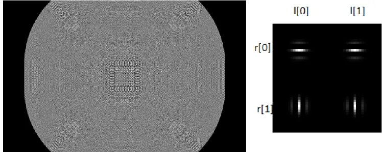
We perform the numerical reconstruction of the cube described in the previous section. Reconstruction is done by using the angular spectrum method on tilted planes as shown in (13_{). We perform the Morlet transform of}

the hologram using the basis function as described in the last section. The Figure(6) shows the hologram and the Morlet function. The Morlet transform is carried out on a Matlab implementation using CUDA. The time taken for the transform is about 1 second on a Quadro 3000M GPU.

The results of the various edges using the appropriate morlet transformed holograms is given in the Figures(7)(8)(9)(10). We show that we are able to reconstruct the edges of the cube from a spare set of Morlet transformed coefficients.

Let us now attempt to reconstruct the FT edge with r[1] and l[1] instead of r[0] and l[0]. The Figure(11) shows the results. Notice how the output loses the sharpness.

6. CONCLUSION

Morlet transformed coefficients are shown to be used in conjunction with a view-based representation system. We have shown the design, discretization and implementation of Morlet wavelets for the view-dependent compression system in detail. Due to a limited number of view-points and the utilization of GPU processing, the speed of the transform is satisfactory. Further to this, the Morlet transformed coefficients can be transmitted based on the position of the viewer for adaptive reconstruction. At each viewer position the overall entropy of the complex hologram field reduces as compared to the whole hologram. In the future we intend to employ efficient entropy coding techniques to reduce the overall bitrate.

Figure 6. Cube hologram (1920x1200px) and morlet wavelets (20x20px)

Figure 7. (Left)Reconstruction of Morlet transformed hologram for r[1] and l[0]. FL edge visible.(Right)Numerical recon-struction of the FL edge

Figure 8. (Left)Reconstruction of Morlet transformed hologram for r[0] and l[0]. FT edge visible.(Right)Numerical recon-struction of the FT edge

Figure 9. (Left)Reconstruction of Morlet transformed hologram for r[0] and l[1]. RR edge visible.(Right)Numerical recon-struction of the RR edge

Figure 10. (Left)Reconstruction of Morlet transformed hologram for r[1] and l[1]. RB edge visible.(Right)Numerical reconstruction of the RB edge

Figure 11. (Left)Reconstruction of Morlet transformed hologram for r[0] and l[0]. FT edge visible.(Center)Numerical reconstruction of the FT edge. (Left)Reconstruction of Morlet transformed hologram for r[1] and l[1]

APPENDIX A. ELIMINATION OF THE DC TERM

g(x) = K.w(βx).s(x) (33)

The fourier transform is given as,

ˆ

g(f ) = K βW (

f

β) (34)

We need to remove the magnitude at f=0. Hence we subtract the output of a low pass Gaussian filter. The low pass filtered output and its fourier transform is given as:

h(x) = g(x) − c.w(βx) (35a) ˆ h(f ) = ˆg(f ) − c βw(ˆ f β) (35b) At f = 0 ˆ g(0) = c βw(ˆ 0 β) (36) Therefore, c = βˆg(0) (37a) = βK βw(ˆ f0 β ) (37b) Substituting, h(x) = K.w(βx).s(x) − K. ˆw(f0 β ).w(βx) (38a) = K.w(βx)[s(x) − ˆw(f0 β)] (38b)

The fourier transform of the gaussian function is given as

ˆ

w(f ) = exp(−π2f2). (39)

Therefore for the 1D form the DC term comes out to be,

ˆ w(f0 β ) = exp(− π2 β2f 2 0) (40)

ACKNOWLEDGMENTS

The authors would like to thank Prof. Levent Onural (Bilkent University) for the fruitful discussions on Gabor basis functions.

REFERENCES

1. E. Darakis and T. J. Naughton, “Compression of digital holograms sequences using mpeg-4,” Proc. of SPIE 7358, March 2009.

2. Y. Xing, B. Pesquet-Popescu, and F. Dufaux, “Compression of computer generated hologram based on phase shifting algorithm,” EUVIP 47, pp. 172–177, 2013.

3. A. Schwerdtner, R. Hussler, and N. Leister, “Large holographic displays for real-time applications,” Journal of Display Technology 6912, January 2008.

4. K. Viswanathan, P. Gioia, and L. Morin, “Wavelet compression of digital holograms:towards view-dependent frameworks,” Proc. SPIE 8856, Applications of Digital Image Processing XXXVI, pp. 1–10, September 2013.

5. T. S. Lee, “Image representation using 2d gabor wavelets,” IEEE transaction on Pattern Analysis and Machine Learning 18, pp. 1–13, october 1996.

6. J. Han and K. K. Ma, “Rotation-invariant and scale-invariant gabor features for texture image retrieval,” Image and Vision Computing 25, pp. 1474–1481, 2007.

7. J. Zhong and J. Weng, Holography, Research and Technologies, Prof. Joseph Rosen (Ed.), Intech Open, 2011.

8. I. Daubechies and F. Planchon, “Adaptive gabor transforms,” Applied Computation Harmony Analysis 13, pp. 1–21, 2002.

9. O. Christensen, “Frames, riesz bases, and discrete gabor/wavelet expansions,” bulletin of American Mathe-matical Society 38, pp. 273–291, March 2001.

10. D. T. L. Lee and A. Yamamoto, “Wavelet analysis: Theory and applications,” Hewlett-Packard Journal 13, pp. 44–54, 1994.

11. J. Morlet, G. Arens, E. Fourgeau, and D. Giard, “Wave propagation and sampling theory part 1: Complex signal and scattering in multi-layered media,” Society of exploration Geo-physicists 47, pp. 203–221, 1982. 12. J. Ashmead, “Morlet wavelets in quantum mechanics,” Quanta 1, pp. 58–70, November 2012.

13. G. B. Esmer, “Computation of holographic patterns between tilted planes,” Master’s thesis, Bilkent Uni-versity, 2004.