HAL Id: hal-02987638
https://hal.archives-ouvertes.fr/hal-02987638
Submitted on 4 Nov 2020
HAL is a multi-disciplinary open access
archive for the deposit and dissemination of
sci-entific research documents, whether they are
pub-lished or not. The documents may come from
teaching and research institutions in France or
abroad, or from public or private research centers.
L’archive ouverte pluridisciplinaire HAL, est
destinée au dépôt et à la diffusion de documents
scientifiques de niveau recherche, publiés ou non,
émanant des établissements d’enseignement et de
recherche français ou étrangers, des laboratoires
publics ou privés.
A Centralized Controller for Reliable and Available
Wireless Schedules in Industrial Networks
Remous-Aris Koutsiamanis, Georgios Papadopoulos, Bruno Quoitin, Nicolas
Montavont
To cite this version:
Remous-Aris Koutsiamanis, Georgios Papadopoulos, Bruno Quoitin, Nicolas Montavont. A
Central-ized Controller for Reliable and Available Wireless Schedules in Industrial Networks. MSN 2020 :
16th International Conference on Mobility, Sensing and Networking, Dec 2020, Virtual, Japan.
pp.1-9, �10.1109/MSN50589.2020.00018�. �hal-02987638�
A Centralized Controller for Reliable and Available
Wireless Schedules
in Industrial Networks
Remous-Aris Koutsiamanis
†, Georgios Z. Papadopoulos
†, Bruno Quoitin
‡and Nicolas Montavont
†† IMT Atlantique, IRISA, France
Email: {firstname.lastname}@imt-atlantique.fr
‡ University of Mons (UMONS), Belgium
Email: [email protected]
Abstract—This paper describes our work on a flexible cen-tralized controller for scheduling wireless networks. The context of this work encompasses wireless networks within the wider Internet of Things (IoT) field and in particular addresses the requirements and limitations within the narrower Industrial In-ternet of Things (IIoT) sub-field. The overall aim of this work is to produce wireless networking solutions for industrial applications. The challenges include providing high reliability and low latency guarantees, comparable to existing wired solutions, within a noisy wireless medium and using generally computationally- and energy-restrained network nodes. We describe the development of a centralized controller for Wireless Industrial Networks, currently aimed at IEEE Std 802.15.4-2015 Time Slotted Channel Hopping protocol. Our controller takes a high-level network-centric problem description as input, translates it to a low-level representation and uses that to retrieve a solution from a Satisfiability Modulo Theories (SMT) solver, translating the solution back to a higher-level network-centric representation. The advantages of our solution are the ability to gain the added flexibility, higher ease of deployment, and lower deployment cost offered by wireless networks by generating configurable and flexible schedules for these applications.
Index Terms—Internet of Things, IoT, Industrial IoT, IEEE Std 802.15.4-TSCH, RAW, ROLL, PAREO Functions, Controller, Scheduling, Resource Allocation
I. INTRODUCTION
Industry 4.0 is expected to rely more and more on Internet of Things (IoT) to make the manufacturing process automated, autonomous, robust and reconfigurable. The IoT has reached a maturity level which makes it possible to consider adapting these technologies for industrial-type applications (e.g., urban deployment, building management, automation and control loops). Different IoT protocols allow IPv6 to be implemented directly on objects, which gives access to a stable and proven environment for exchanging data. Thus, by employing IP technologies, cost reduction and reliable communication is achieved [1].
Scenarios such as smart grid or factory automation where the product can be, for instance, vehicles, require Low-power and Lossy Networks (LLNs) that consist of hundreds of sensors and actuators communicating with an LLN Border Router (LBR) [2], [3]. However, in order to extend the network beyond the radio coverage of one node, a mesh technology
allows a node to act as a relay for others, but, beyond one hop, a protocol is required for routing packets through the multi-hop network. Note that the constrained devices with limited memory and processing resources can be interconnected by a variety of links, such as IEEE Std 802.15.4, Low Power WiFi or Power Line Communication (PLC) links. LLNs are transitioning to an end-to-end IP-based solution to allow inter-operability across the networks. To enable and manage such an interconnection, we use the IPv6 Routing Protocol for Low-Power and Lossy Networks (RPL), one of the most adopted routing protocols for the IoT. RPL has been standardized in the Internet Engineering Task Force (IETF) Routing Over Low power and Lossy networks (ROLL) Working Group (WG) and is adapted to noisy wireless environments and also takes into consideration the computational, memory, and energy constraints of battery-operated network nodes.
In 2016, the IEEE Std 802.15.4-2015 TSCH was pub-lished. Time Slotted Channel Hopping (TSCH) uses Time-Division Multiple Access (TDMA) and Frequency-Hopping Spread Spectrum (FHSS) techniques to achieve high network reliability, to reduce energy consumption and to mitigate multi-path fading as well as external interference. To do so, TSCH employs a strict schedule of non-interfering transmissions and supports using both centralized and distributed scheduling algorithms, i.e., Scheduling Functions, to allocate a certain number of resources to each node for transmission opportuni-ties. However, the standard defines how the Medium Access Control (MAC) executes a schedule but not how such a schedule is built.
In this work, we aim to approximate deterministic network communications, as much as possible. While it is fundamen-tally impossible to achieve fully deterministic communications due to the probabilistic and relatively lossy nature of the wireless medium, our goal is nevertheless to provide high-enough reliability and latency guarantees. We describe the centralized controller that we have developed to address the previously presented challenges while providing flexibility in adding further features. As a result, in addition to supporting standard IEEE Std 802.15.4-2015 TSCH schedule features, we also support not-yet standardized features, such as
promiscu-ous overhearing and multi-path routing [4], which allow the development of high reliability LLNs.
In the rest of this paper, the required technical background as well as the related work are presented in Section II. Afterward, in Section III we present the operation and features of the controller and in Section IV the specification of its operation. We then describe the experimental setup with the parameters evaluated and performance metrics analyzed in Section V, and we present the results in Section VI. Finally, we conclude with potential future work in Section VII.
II. TECHNICALBACKGROUND ANDRELATEDWORK
In this section, we first present the default operations of the IEEE std 802.15.4-2015 TSCH and RPL standards. Then, we give an overview of the Satisfiability Modulo Theories (SMT) solvers and the Haskell SBV library used to express and solve the scheduling problem. Finally, we describe some key scheduling algorithms from the literature.
A. IEEE std 802.15.4-2015 TSCH
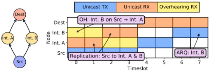
In TSCH, a communication schedule and time synchroniza-tion are employed to accurately choreograph the transmissions and receptions between nodes [5]. An example of a TSCH schedule for a small network topology is shown in Figure 1.
More specifically, in a TSCH network, time is divided into timeslots of equal length (the standard proposes 10ms), sufficient enough to transmit a data packet and to receive an ac-knowledgement. If the acknowledgment is not received within the timeslot duration, the retransmission of the packet will be delayed to one of the following timeslots depending on the defined schedule. At each timeslot, each node is aware whether it has to stay “awake” (i.e., radio on) in order to transmit or receive a packet, or to “sleep” (radio off) to save energy. Next, a set of timeslots constructs a slotframe, of configurable size, that repeats perpetually. The nodes synchronize the start of their slotframe based on Enhanced Beacon (EB) control packets.
Furthermore, the timeslots are identified by an Absolute Slot Number (ASN) counter that increments as time elapses; the ASN actually counts the number of timeslots since the establishment of the TSCH network. All nodes in the network are aware of the current ASN value and therefore are time-synchronized in this manner.
To define a TSCH schedule, for each pair of nodes (i.e., radio link) a set of cells that consists of timeslots and channel offsets is assigned. A channel offset is a “virtual channel” that is translated into a physical radio channel that is going to be employed for communication.
1) Route Computation: Path computation can be achieved
in a centralized manner, e.g., each node requests from a Path Computation Element (PCE) for new cells to use. The advantage is that the PCE can be flexibly positioned, either on the network backbone or farther away in the IPv6 network over a back-haul Additionally, the computation resources available to calculate the schedule are much higher since the device is not constrained the same way the IoT devices are.
Src
Int. A Int. B
Dest Unicast TX Unicast RX Overhearing RX
0 1 2 3 4 5 6 7 Timeslot Src Int. A Int. B Dest Node ARQ: Int. B OH: Int. B on Src Int. A
ARQ: Int. B OH: Int. B on Src Int. A
Replication: Src to Int. A & B
Fig. 1. Topology and schedule in a TSCH/RPL network, showing unicast TX and RX, ARQ and Overhearing.
One of the first centralized schedulers for this domain, TASA [6], uses graph theory to explore the network graph and produce a schedule with high compactness in order to make efficient network resource allocation. In order to address unreliable links, a method of over-provisioning additional cells is also proposed [7]. Another scheduler, ASchedEx [8], allows customized cell allocation to different flows in the network, thus affording a different number of transmission opportunities to different flows. At the same time it allows specifying and observing end-to-end delay constraints.
While these schedulers provide useful features, it is hard to extend their functionality when new features are desired since they are purpose-built. The controller proposed in this paper uses a direct, high-level, and network-centric problem formu-lation to express the scheduling problem. Since the problem-solving mechanism is abstracted away, with our controller it is comparatively easier to add new features and constraints. For example, packet transmission reliability can be increased by performing multi-path routing [9]. This feature is simple to implement in our controller but may require a full redesign with fixed-function schedulers.
However, centralized algorithms need a precise view of the network conditions, and generate a large overhead when the schedule has to be updated. Alternatively, the route com-putation can be done in a distributed manner, where the nodes are employing a hysteresis function to decide how many cells to (de)allocate [10]. In this work, we focus on a centralized algorithm for the IIoT use case, assuming that the network requirements are reasonably stable and can be retrieved directly from the network operator or by gathering statistics and recalculating the schedule periodically.
2) Track: A track corresponds to dedicated radio resources,
along with a multi-hop path. More precisely, a set of cells (a bundle) is reserved for each hop. Different tracks use a different set of cells (i.e., different timeslots and/or channels), thus providing traffic isolation. A track forwarding scheme is applied: when a node receives a frame to forward, it automatically finds the outgoing cells associated with the incoming cells. In Figure 2, the flow from A to the border router R, via node B, will be assigned to track 1, while the same node (e.g., B) may forward an additional flow, for instance from C, using a different track (i.e., 2). Since each cell is associated with one single track, label switching can be used: when a packet is received during a cell labeled with a given track, the node can forward the packet only during a
A B R C track radio link in the DODAG slotframe track 1 track 2 dedicated cells 4 3 A▶︎B B▶︎R A▶︎B B▶︎R 2 1 channel offset shared cells B▶︎R B▶︎R C▶︎B … … unused cells 0
Fig. 2. Schedule in a RPL/TSCH network, using two different tracks for
traffic isolation.
Fig. 3. Example of a DAG and a DODAG.
cell with the same track label.
B. RPL networks
RPL [11] is a link-layer agnostic distance vector routing protocol. In the wireless networks which we are addressing, the topology is not predefined and, thus, RPL is in charge of discovering and carefully selecting nodes in order to construct optimal routes.
The topology is organized based on a Directed Acyclic Graph (DAG), a graph where the connections between nodes have a direction and an acyclic (non-circular) property. In Figure 3 (a), a DAG composed of ten nodes and three DAG roots is illustrated. To construct a routing topology, RPL employs a Destination-Oriented Directed Acyclic Graph (DODAG), a DAG restricted to a single root. Thus, the graph comprises at least one root, a node with no outgoing edge, typically acting as a gateway to an external network. Figure 3 (b) depicts a DODAG topology that consists of eight nodes with one root.
RPL requires link-layer resources to perform packet for-warding. In this work, the scheduler allocates a super-set of the resources required by RPL, and RPL will decide on-demand which subset of the resources it will use by making the routing decisions.
C. RAW and PAREO Functions
At the IETF, a new direction is being considered over wire-less communication, called Reliable and Available Wirewire-less (RAW) [12]. The RAW WG focuses on layer-3 and will operate over a wide range of schedule-based radios, such as IEEE std 802.15.4-2015 TSCH, 5G and WiFi 6 [13]. The RAW WG considers the forwarding operation along a track, as mostly a DODAG toward a root destination, with potential parallel links and paths for enhanced reliability, and possibly heterogeneous technologies along the path. RAW is applying the concept of Packet Automatic Repeat reQuest (ARQ), Replication and Elimination (RE), and Overhear-ing (PAREO) functions to provide an acceptable trade-off of energy and bandwidth versus reliability and availability over wireless industrial network [4]. More specifically, the Replication function duplicates the data packets over multiple paths in the network to increase reliability and minimize jitter. Since the replication mechanism introduces additional traffic in the network, the Elimination function is used to remove unnecessary duplication. To eliminate duplicates, a way of identifying packets is required and usually some type of tag is used as part of the packet header. Then, the ARQ function is used as a complement to further increase end-to-end reliability by retransmitting up to a maximum count if the previous transmissions failed.
Finally, the promiscuous Overhearing function is used to take advantage of the wireless medium by allowing multiple nodes to receive the same packet with one transmission if the receiver nodes are all within listening range of the transmission. This allows spending less time and energy than individual transmissions toward each listener.
D. SMT solvers and SBV
In this work, we use an SMT solver to support flexi-ble and general constraints for generating TSCH schedules. SMT solvers are tools which solve a more general class of problems than Boolean Satisfiability (SAT). They allow the fully automatic solving of the satisfiability of first-order theories including arithmetic equations and inequalities, with existential and universal quantification as well as support-ing non-linear functions such as minimum and maximum. They are normally used for smaller problems, but recently it has become feasible to use these tools for scheduling-type problems [14]. In this work, the Z3 solver [15] is used, but the architecture of the controller allows the easy substitution of this solver with any solver supported by the SMT-LIB
2.0 library1. To make it possible to define the problem and
the constraints on the solution in a high-level and network-centric way, we use the Haskell programming language and its SBV library to automatically and bidirectionally translate the problem from the high-level constructs to the lower-level SMT-LIB 2.0 format that the solver uses. The SBV library provides variable types (e.g., unsigned and signed integers of different bit lengths, booleans) and the ability to bind variables with
constraints (e.g., one variable needs to be less than another). The set of variables and constraints are sent through a number of transformations to the SMT solver to be automatically solved like any other supported problem. If there is a solution, the solver returns a set of assignments of values to variables, which observe the constraints.
III. SYSTEMOPERATION ANDFEATURES
A. System Operation
The operation of the system comprises five steps:
1) The end-user defines the problem to be solved at a high-level via a problem abstraction (see Section IV). 2) The problem is automatically converted into a lower-level
representation, but still at the network-level, i.e. TSCH-level concepts like timeslots and channel offsets, and constraints on the combinations permissible to form valid transmission schedules.
3) The lower-level representation then is automatically con-verted to the internal format of the library used to communicate with the SMT solver.
4) The library finally automatically converts the representa-tion to the specific format supported by the SMT solver itself, and sends the input to the solver.
5) The results from the solver follow the reverse path and result in a domain-specific (a TSCH schedule, see Section IV) representation of the SMT solver solution found, if there is a solution. If there is no solution, or a timeout has elapsed, the system assumes that no solution was available for the given problem with the given constraints.
B. Features
The controller currently supports the semantics of TSCH data cells, which are the more complicated ones since they have explicit sender and receiver nodes, and are the ones which mainly affect schedule performance. We support at the end-user abstraction level the definition of upward UDP packet flows (i.e., tracks) at a high level, taking into account over-hearing, packet replication and elimination and MAC-layer retransmission attempts. For each packet sent from one node to another a number of parameters can be individually controlled (see Section IV). The controller output is the schedule in the form of a set of needed TSCH cells to ensure that all data packet transmissions are completed within one slotframe. Additionally, the generated schedule will take advantage of spatial diversity to allow parallel independent transmissions when they do not interfere and channel diversity to allow parallelism when they would interfere due to spatial proximity. C. Implementation
The scheduling problem is described using normal Haskell code. The controller determines which link-layer transmissions need to be performed to support each requested track, taking the topology of the network into account. The aim is to support all potential routes within the schedule and the result is a list of required link-layer communications. For each required
cell, the (unknown) timeslot and channel offset variables are represented using facilities provided by the SBV library (solver variables of unsigned integral 16-bit and 8-bit types correspondingly). Constraints are then set on the variables, e.g., that the timeslot variable of one cell needs to be a lower value (i.e., “before”) the timeslot variable of another cell to express that one transmission needs to be scheduled before another one.
The problem is automatically encoded by SBV into a cross-SMT-solver-compatible format (SMT-lib 2.0) and is given as input to the SMT solver back-end If a solution is available and computed within a given deadline it is then automatically parsed and made available within the Haskell program, to be formatted or used appropriately. Otherwise, the problem is considered unsolvable for our purposes.
While SBV and Z3 allow specifying optimization objec-tives, e.g., “minimize the number of timeslots used”, we have found that the performance trade-off is unsatisfactory when using this feature. Currently therefore, to allow optimization of the schedule for schedule size, we perform a binary search on the maximum timeslots available, yielding an approximate optimal solution within a requested timeslot margin. More specifically, following the binary search algorithm, we request a schedule within an initial timeslot count, and if successful we request another solution with the half of the initial timeslot count. If unsuccessful we double the timeslot count. This process continues until the solution is narrowed down to within a specified margin.
IV. CONTROLLERSPECIFICATION
In this section the input and output of the controller are described as well as the constraints used to generate the schedule.
A. Controller Input
The controller input at the high-level (end-user) consists of:
Cmax: the maximum number of channels available for use
(Cmax ≥ 1).
Tmax: the maximum number of timeslots available for use
(Tmax ≥ 1).
N : the number of nodes in the network, with node IDs belonging to {1 . . . N } (N ≥ 1).
Eu: the upward (toward the root node) edges in the node
reachability graph where i, j ∈ {1 . . . N }, i 6= j and
(i, j) ∈ Eu denotes that node i can send unicast data
to node j and j can receive data from i. The edges need to form an acyclic graph.
ρ: the id of the root node in the network (ρ ∈ {1 . . . N }). P: A set of independent UDP packet transmissions (|P| ≥ 0)
to schedule within the same slotframe. For each k of these the following parameters are given:
PTXk, PRXk: the node PTXk sending the packet
and the node PRXk receiving the packet, where
PTXk, PRXk ∈ {1 . . . N }, PTXk 6= PRXk.
POHk: whether overhearing is enabled for this packet
PNk: the maximum number of MAC layer transmissions
at each hop (PNk≥ 1).
PTk: the timeslot in the slotframe at which the packet
should be sent at the earliest, i.e. earliest time of
availability to send (PTk ≥ 0).
B. Controller Output
The output of the controller is a full TSCH schedule if one is possible given the constraints, or a response indicating a failure to generate a schedule either due to the constraints or due to not enough time to compute a schedule. If a schedule is produced then the result is a set of TSCH cells S, where each cell c is of the form:
SCHc, STSc: the channel offset SCHcand the timeslot STSc
of the cell, where SCHc∈ {0 . . . Cmax− 1} and STSc∈
{0 . . . Tmax − 1}.
STXc, SRXc, SOHc: the node STXc sending the packet at
the TSCH/MAC layer and the node SRXc receiving the
packet at the TSCH/MAC layer, where STXc, SRXc ∈
{1 . . . N }, SOHc ∈ {0 . . . N }, STXc 6= SRXc 6= SOHc.
If this is an overhearing cell, then SRXc contains the
overhearing receiver node and SOHc the intended
re-ceiver of the corresponding non-overhearing
transmis-sion. If it is not an overhearing cell, then SOHc = 0.
SPc: the UDP packet transmission of which this cell is part
of its track, where SPc ∈ P.
SNc: the number of the MAC layer transmission that this cell
represents, where SNc∈ {1 . . . PNSPc}.
C. Controller Variables and Constraints
To construct a problem for the SMT solver, the controller takes the high-level input and constructs a number of variables and constraints on the values of those variables. More specif-ically, it creates the set S of cells, but out of the properties of
each cell c, only the SCHc and the STSc properties are
con-figured as solver variables. Effectively, the solver constructs all the needed cells for the packet transmission given the problem
high-level input and only sends the SCHc and STScvariables
to the solver, accompanied by a set of constraints on the values of these variables.
The controller generates the following constraints:
• Support single radio devices: Nodes can only transmit or
receive data on up to one channel in each timeslot.
• Support multi-hop forwarding: The forwarding of a
packet must happen after the reception of a packet.
• Support PRE: All the potential copies/replicas of a UDP
packet arriving via any child to a node must be received before starting to forward to the next-hop node(s).
• Support ARQ: All the MAC layer transmissions of a UDP
packet arriving via any child to a node must be received before staring to forward to the next-hop node(s).
• Support Overhearing: When a node is overhearing a
trans-mission, it must do so on the same timeslot and channel offset as the corresponding non-overhearing transmission.
1 2 3 4 5 6 7 8
Fig. 4. Linear topology with one parent per node and 8 layers.
• Reduce latency and jitter: Consecutive packet MAC layer
transmissions (on the same link) must happen on consec-utive timeslots.
If there is more than one upward edge from node i, i.e.,
|{v|(i, v) ∈ Eu}| > 1, then for each receiver a separate cell
will be created. This allows implementing packet replica-tion and overhearing. If overhearing is enabled for a packet
(POHk = True), all the potential parents in each upward
link on the upward path will be set to overhearing. More specifically, given a link from node i to node j, the rest of the potential receivers of node i, except for j, i.e., {v|(i, v) ∈
Eu, v 6= j}, will be set to overhear the transmission.
V. EXPERIMENTALSETUP
A. Tools
The controller is implemented in Haskell and is compiled using GHC (8.6.5). The Haskell code uses the SBV (8.5.5) library to translate to the SMT-LIB 2.0 format and solves the scheduling problems using the Z3 (4.8.8) SMT back-end solver, but other ones (e.g., Yices 2, MathSAT 5) can also be used. The hardware used is one core of an Intel Xeon Gold 6130 CPU with 8 GB of RAM dedicated to each controller process generating one schedule. The operating system used is Debian Linux 10, 64-bit.
B. Evaluation Parameters
This section describes which parameters were used in the experimental performance evaluation of the controller. In total, 54 different schedules were generated and presented from all the parameter combinations.
1) Topologies: Three network topologies with single-path
and multi-path configurations are used to evaluate the con-troller’s schedule generation capabilities. The UDP packets are always requested to be sent at timeslot 0 at the earliest
(∀p ∈ P, PTp = 0) and the destination is always the root
node, node 1 (∀p ∈ P, PRXp = 1). The source nodes of the
UDP packets are the leaf nodes; the intermediate nodes always forward packets originating in the leaves, but don’t generate their own packets.
a) Linear Topology: Firstly, the linear topology of N
nodes is illustrated in Figure 4 for N = 8. The last node (node N in general, node 8 in Figure 4) sends one packet to the root node (node 1) per slotframe. In this topology,
only one TSCH channel is used (Cmax = 1) since channel
diversity is not possible or useful due to the structure of the network. We evaluate schedule generation for topologies with N ∈ {5, 9, 17, 33, 65} and N − 1 hops.
b) Binary Topology: Secondly, the perfect binary
topol-ogy of N nodes is illustrated in Figure 5 for N = 7 and 3 layers. The nodes in the last layer (nodes [(N + 1)/2, . . . , N ] in general, nodes 4-7 in Figure 5) send one packet to the root
1
2 3
4 5
6 7
Fig. 5. Binary-tree-like topology with two parents per node and three layers.
1
2 3 4
5 6 7 11 12 13 8 9 10
Fig. 6. Ternary-tree-like topology with two parents per node and three layers.
node (node 1) per slotframe. In this topology, all 16 TSCH
channels are available (Cmax = 16) to evaluate the ability of
taking advantage of channel diversity. Additionally, each node,
with the exception of the 2ndlayer (nodes 2, 3) can have either
one or two potential parents in their parent set. We evaluate the creation of both single-path tracks (where only one of the parents is used for forwarding packets) and dual parent-tracks where the tracks contain cells to replicate the packet to both parents. Finally, binary topologies with 3, 4, 5, and 6 layers, i.e., N ∈ {7, 15, 31, 63}, are evaluated.
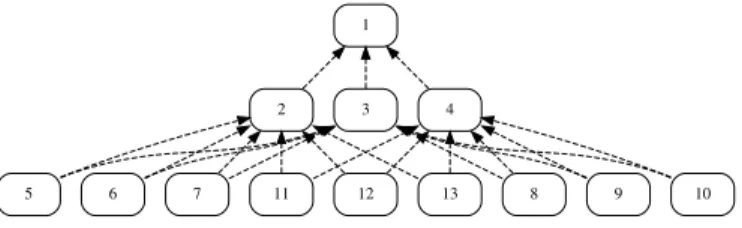
c) Ternary Topology: Finally, the perfect ternary
topol-ogy of N nodes is illustrated in Figure 6 for N = 13 and 3 layers with two parents in the parent set of the nodes. The nodes in the last layer (i.e., nodes [2(N + 2))/3, . . . , N ] in general, nodes 5-13 in Figure 6) send one packet to the root node (node 1) per slotframe. In this topology, as with the
binary one, all 16 TSCH channels are available (Cmax = 16)
to evaluate the ability of taking advantage of channel diversity.
Additionally, each node, with the exception of the 2nd layer
(nodes 2, 3, 4), can have either one, two, or three potential parents in their parent set. Similarly to the binary topology, we evaluate the creation of both single-path tracks as well as dual-path and triple-path tracks. Finally, ternary topologies with 3 and 4 layers, i.e., N ∈ {13, 40}, are evaluated.
2) MAC-layer transmissions: We evaluate schedule
gener-ation with one MAC-layer transmission (i.e., no
retransmis-sions, ∀p ∈ P, PNp = 1) as well as with two MAC-layer
transmissions (i.e., one retransmission, ∀p ∈ P, PNp = 2)
per link. When two transmissions are used, the cells for the transmissions are required to be in adjacent timeslots to reduce latency and jitter.
3) Overhearing: We evaluate schedule generation with
(∀p ∈ P, POHp = T rue) and without (∀p ∈ P, POHp =
F alse overhearing. Since overhearing only makes sense with multiple parents, in the cases where the parameters of the topology specify single-path tracks overhearing is not eval-uated.
4) Schedule size optimization - Binary search: For the
binary search of a minimally sized schedule, we start the
binary search at 1250 timeslots (Tmax = 1250) and use a
maximum of 2500 timeslots (Tmax = 2500) for the upper
bound of the binary search, which is the approximate num-ber of cells in the most complicated example. We continue searching for solutions until the timeslot margin in the binary search algorithm is less than or equal to 5 timeslots (to reduce scheduling time spent for little gain) and we allocate up to 30 minutes per binary search step for finding for a solution.
VI. PERFORMANCEEVALUATIONRESULTS
The results overall show that the proposed controller is a viable solution for small and medium sized TSCH networks with very complicated and demanding traffic requirements. We measure and present the following interesting aspects of our controller’s schedule generation.
A. Total Schedule Computation Time
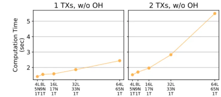
This measure expresses the time required for all the binary search steps to retrieve a final schedule. The results, presented in Figure 7, 8 and 9, show that medium size networks up to 63 nodes (in the binary topology) are supported with quite high traffic requirements (2 MAC-layer transmissions, dual-path tracks, overhearing and 32 leaf nodes sending packets). The linear topology shows that for simple topologies the computation time is negligible and scales approximately with the number of nodes N and the number of MAC-layer
transmissions PNk, as expected.
Additionally, it can be seen that for the binary and ternary topologies, the time required scales with the total number of cells in the schedule. Using multi-path tracks, overhearing and multiple retransmissions all have an impact on the time required. It is noteworthy that in all cases the time required is under 3 hours, allowing the controller to be used realisti-cally in a recompute-at-night fashion, after gather statistical information throughout the day.
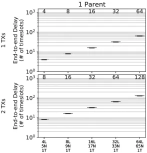
B. End-to-end latency
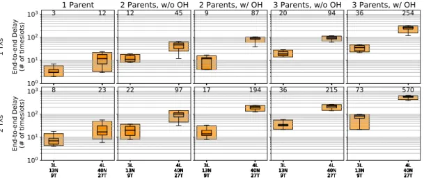
The time in timeslots required for a packet (potentially with retransmissions, overhearing and multi-path tracks) to traverse the network, from a sending node in the last layer to the root node is an important metric of the efficiency of the schedule. The results, presented in Figure 10, show as expected no variability in the linear topology and the correct number of timeslots used. For the binary and ternary topologies, the results show, in Figure 11 and 12, an exponential scaling of latency with the number of layers in the topology, as expected, since the number of sending nodes also increases exponentially with the number of layers. In all cases, the latency is kept under 700 timeslots, despite having to schedule over 2000 cells in the more high-traffic cases.
While some variability in the end-to-end latency of different packets exists, we have not requested any special treatment for any packet. It would easily be possible to request more specific maximum end-to-end latency values for specific UDP packet
4L 5N 1T 8L 9N 1T 16L 17N 1T 32L 33N 1T 64L 65N 1T 2 3 4 5 Computation Time (sec)
1 TXs, w/o OH
4L 5N 1T 8L 9N 1T 16L 17N 1T 32L 33N 1T 64L 65N 1T2 TXs, w/o OH
Fig. 7. Results for the total schedule computation time required for the linear topology, expressed in seconds. The notation xL, yN, zT refers to the number of layers, total nodes and sending leaf nodes correspondingly.
transmissions, just by constraining the maximum number of allowed timeslots between the packet’s first and last cell in the track.
C. Used timeslots
The number of timeslots in the schedule that are used, i.e., the length of the slotframe, is an indication of how compact the schedule generated is. The results for the linear topology are omitted since due to the use of the linear topology and just one channel the length of the slotframe is the same as the end-to-end latency. For the binary and ternary topologies, the results, shown in Figure 15 and 16, indicate a strong correlation with the maximum end-to-end latency, thus meaning that the controller is able to schedule cells in parallel in order not to increase the slotframe size. As with end-to-end latency, in all cases, the total slotframe length is kept under 700 timeslots. D. Channel utilization
Another indicator of the ability of the controller to take advantage of channel diversity is channel utilization. It is expressed as the number of channels used per timeslot in the schedule and it is variable since different timeslots in the schedule have different numbers of channels used. The results for the linear topology are omitted since only channel is used. For the binary and ternary topologies, the results, shown in Figure 13 and 14, reveal that it is possible to take advantage of channel diversity as the number of parents and the number of MAC-layer transmission increases, reaching a maximum of 10 parallel channels utilized. However, the results also show that the use of overhearing severely restricts this ability, which is expected since overhearing requires all parents to be listening at the same time, therefore limiting other nodes in the parent’s neighborhood from also transmitting. However, a wider network topology might afford more opportunities for parallelizing overhearing-enabled transmissions.
VII. CONCLUSION
This work trades off flexibility and extensibility for some computational limitations. Traditionally, specialized or semi-specialized scheduling algorithms have been used to solve scheduling problems. Fortunately, the use of modern general purpose SMT solvers offers additional flexibility in terms of
3L 7N 4T 4L 15N 8T 5L 31N 16T 6L 63N 32T 0 2500 5000 7500 10000 Computation Time (sec) 1 TXs, w/o OH 3L 7N 4T 4L 15N 8T 5L 31N 16T 6L 63N 32T 1 TXs, w/ OH 3L 7N 4T 4L 15N 8T 5L 31N 16T 6L 63N 32T 2 TXs, w/o OH 3L 7N 4T 4L 15N 8T 5L 31N 16T 6L 63N 32T 2 TXs, w/ OH 2 Parents 1 Parent
Fig. 8. Results for the total schedule computation time required for the binary topology, expressed in seconds.
3L 13N 9T 4L 40N 27T 0 2500 5000 7500 10000 Computation Time (sec) 1 TXs, w/o OH 3L 13N 9T 4L 40N 27T 1 TXs, w/ OH 3L 13N 9T 4L 40N 27T 2 TXs, w/o OH 3L 13N 9T 4L 40N 27T 2 TXs, w/ OH 2 Parents 3 Parents 1 Parent
Fig. 9. Results for the total schedule computation time required for the ternary topology, expressed in seconds.
the class of expressible constraints as well as much better performance than past SMT solver options. However, the trade-off remains and using such a general approach will come with limitations on the size of the problems which are solvable. It is therefore very useful to have realistic network examples available for testing to gauge the applicability of this approach and to propose previously impossible constraints, which might offer unique scheduling features. For example, the link quality for each node pair can be used to create schedules which increase or decrease the number of replications to adapt to the quality, leading to lower energy consumption on more stable links and to higher reliability on more unstable links. The same information can be used to enable or disable overhearing per link, to allow partial multi-path redundancy. An additional option could constitute producing schedules with latency or jitter minimization goals, even partially (per track), instead of globally.
ACKNOWLEDGMENTS
Experiments presented in this paper were carried out using the Grid’5000 testbed, supported by a scientific interest group hosted by Inria and including CNRS, RENATER and several Universities as well as other organizations (see https://www. grid5000.fr). Additionally, this work was partially performed and supported under the TPI ANR-17-CE10-0007-01 project of the French National Research Agency.
REFERENCES
[1] G. Z. Papadopoulos, P. Thubert, F. Theoleyre, and C. Bernardos, “RAW Use Cases,” IETF I-D draft-bernardos-raw-use-cases-01, Nov. 2019. [2] K. Pister, P. Thubert, S. Dwars, and T. Phinney, “Industrial Routing
Requirements in Low-Power and Lossy Networks,” IETF, RFC 5673, 2009.
10
010
110
210
31 TXs
End-to-end Delay (# of timeslots)
4
8
1 Parent
16
32
64
4L 5N 1T 8L 9N 1T 16L 17N 1T 32L 33N 1T 64L 65N 1T 4L 5N 1T 8L 9N 1T 16L 17N 1T 32L 33N 1T 64L 65N 1T10
010
110
210
32 TXs
End-to-end Delay (# of timeslots)
8
16
32
64
128
Fig. 10. Results for the end-to-end latency of packets send from the last layer of the linear topology. Time in TSCH timeslots, from the first packet TX at the sender, to the last copy RX at the root. In each plot, the outer (lighter) box corresponds to the 5%-95% percentiles, the inner (darker) to the 25%-75% percentiles, the middle line to the median and the whiskers represent the minimum and maximum. On top of each box, the mean value is presented.
100
101
102
103
1 TXs
End-to-end Delay (# of timeslots)
3
1 Parent
7 9 202 Parents, w/o OH
5 23 50 109 92 Parents, w/ OH
36 96 2023L 7N 4T 4L 15N 8T 5L 31N 16T 6L 63N 32T 3L 7N 4T 4L 15N 8T 5L 31N 16T 6L 63N 32T 3L 7N 4T 4L 15N 8T 5L 31N 16T 6L 63N 32T 3L 7N 4T 4L 15N 8T 5L 31N 16T 6L 63N 32T 3L 7N 4T 4L 15N 8T 5L 31N 16T 6L 63N 32T 3L 7N 4T 4L 15N 8T 5L 31N 16T 6L 63N 32T 100 101 102 103 2 TXs
End-to-end Delay (# of timeslots)
7 14 20 34 3L 7N 4T 4L 15N 8T 5L 31N 16T 6L 63N 32T 3L 7N 4T 4L 15N 8T 5L 31N 16T 6L 63N 32T 3L 7N 4T 4L 15N 8T 5L 31N 16T 6L 63N 32T 3L 7N 4T 4L 15N 8T 5L 31N 16T 6L 63N 32T 3L 7N 4T 4L 15N 8T 5L 31N 16T 6L 63N 32T 3L 7N 4T 4L 15N 8T 5L 31N 16T 6L 63N 32T 12 36 107 257 3L 7N 4T 4L 15N 8T 5L 31N 16T 6L 63N 32T 3L 7N 4T 4L 15N 8T 5L 31N 16T 6L 63N 32T 3L 7N 4T 4L 15N 8T 5L 31N 16T 6L 63N 32T 3L 7N 4T 4L 15N 8T 5L 31N 16T 6L 63N 32T 3L 7N 4T 4L 15N 8T 5L 31N 16T 6L 63N 32T 3L 7N 4T 4L 15N 8T 5L 31N 16T 6L 63N 32T 21 81 192 515
Fig. 11. Results for the end-to-end latency of packets send from the last layer of the binary topology. Time in TSCH timeslots, from the first packet TX at the sender, to the last copy RX at the root. In each plot, the outer (lighter) box corresponds to the 5%-95% percentiles, the inner (darker) to the 25%-75% percentiles, the middle line to the median and the whiskers represent the minimum and maximum. On top of each box, the mean value is presented.
[3] F. Lemercier, G. Habault, G. Z. Papadopoulos, P. Maille, P. Chatzimisios, and N. Montavont, “Communication Architectures and Technologies for Advanced Smart Grid Services,” in Transportation and Power Grid in Smart Cities: Communication Networks and Services, M. H. R. Hussein T. Mouftah, Melike Erol-Kantarci, Ed. Wiley, 2018, ch. 8, pp. 217–246. [4] R.-A. Koutsiamanis, G. Z. Papadopoulos, T. Lagos Jenschke, P. Thubert, and N. Montavont, “Meet the PAREO Functions: Towards Reliable and Available Wireless Networks,” in Proceedings of the IEEE International Conference on Communications (ICC), 2020.
[5] “IEEE Standard for Low-Rate Wireless Personal Area Networks (LR-WPANs),” IEEE Std 802.15.4-2015, April 2016.
[6] M. R. Palattella, N. Accettura, L. A. Grieco, G. Boggia, M. Dohler, and T. Engel, “On Optimal Scheduling in Duty-Cycled Industrial IoT Applications Using IEEE802.15.4e TSCH,” IEEE Sensors Journal,
vol. 13, no. 10, pp. 3655–3666, Oct 2013.
[7] G. Gaillard, D. Barthel, F. Theoleyre, and F. Valois, “High-reliability scheduling in deterministic wireless multi-hop networks,” in PIMRC. IEEE, Sep. 2016, pp. 1–6.
[8] F. Dobslaw, T. Zhang, and M. Gidlund, “End-to-End Reliability-Aware Scheduling for Wireless Sensor Networks,” IEEE Transactions on In-dustrial Informatics, vol. 12, no. 2, pp. 758–767, April 2016. [9] R.-A. Koutsiamanis, G. Z. Papadopoulos, X. Fafoutis, J. M. Del Fiore,
P. Thubert, and N. Montavont, “From Best Effort to Deterministic Packet Delivery for Wireless Industrial IoT Networks,” IEEE Transactions on Industrial Informatics, vol. 14, no. 10, pp. 4468–4480, Oct 2018. [10] T. Chang, T. Watteyne, X. Vilajosana, and Q. Wang, “CCR:
Cost-aware cell relocation in 6TiSCH networks,” Transactions on Emerging Telecommunications Technologies, vol. 29, no. 1, p. e3211, 2018. [11] T. Winter, P. Thubert, A. Brandt, J. Hui, R. Kelsey, P. Levis, K. Pister,
R. Struik, J. Vasseur, and A. R., “RPL: IPv6 Routing Protocol for Low-Power and Lossy Networks,” IETF RFC 6550, 2012.
[12] P. Thubert and G. Papadopoulos, “Reliable and Available Wireless Problem Statement,” IETF, I-D draft-pthubert-raw-problem-statement-04, Oct. 2019.
[13] P. Thubert, D. Cavalcanti, X. Vilajosana, and C. Schmitt, “Reliable and Available Wireless Technologies,” IETF, Internet-Draft draft-thubert-raw-technologies-03, Jul. 2019.
[14] S. F. Roselli, K. Bengtsson, and K. ˚Akesson, “Smt solvers for job-shop
scheduling problems: Models comparison and performance evaluation,” in 2018 IEEE 14th International Conference on Automation Science and Engineering (CASE), Aug 2018, pp. 547–552.
[15] L. de Moura and N. Bjørner, “Z3: An efficient smt solver,” in Tools and Algorithms for the Construction and Analysis of Systems, C. R.
Ramakrishnan and J. Rehof, Eds. Springer Berlin Heidelberg, 2008,
100
101
102
103
1 TXs
End-to-end Delay (# of timeslots)
3
1 Parent
122 Parents, w/o OH
12 452 Parents, w/ OH
9 873 Parents, w/o OH
20 943 Parents, w/ OH
36 2543L 13N 9T 4L 40N 27T 3L 13N 9T 4L 40N 27T 3L 13N 9T 4L 40N 27T 3L 13N 9T 4L 40N 27T 3L 13N 9T 4L 40N 27T 3L 13N 9T 4L 40N 27T 3L 13N 9T 4L 40N 27T 3L 13N 9T 4L 40N 27T 3L 13N 9T 4L 40N 27T 3L 13N 9T 4L 40N 27T 100 101 102 103 2 TXs
End-to-end Delay (# of timeslots)
8 23 3L 13N 9T 4L 40N 27T 3L 13N 9T 4L 40N 27T 3L 13N 9T 4L 40N 27T 3L 13N 9T 4L 40N 27T 3L 13N 9T 4L 40N 27T 3L 13N 9T 4L 40N 27T 3L 13N 9T 4L 40N 27T 3L 13N 9T 4L 40N 27T 3L 13N 9T 4L 40N 27T 3L 13N 9T 4L 40N 27T 22 97 3L 13N 9T 4L 40N 27T 3L 13N 9T 4L 40N 27T 3L 13N 9T 4L 40N 27T 3L 13N 9T 4L 40N 27T 3L 13N 9T 4L 40N 27T 3L 13N 9T 4L 40N 27T 3L 13N 9T 4L 40N 27T 3L 13N 9T 4L 40N 27T 3L 13N 9T 4L 40N 27T 3L 13N 9T 4L 40N 27T 17 194 3L 13N 9T 4L 40N 27T 3L 13N 9T 4L 40N 27T 3L 13N 9T 4L 40N 27T 3L 13N 9T 4L 40N 27T 3L 13N 9T 4L 40N 27T 3L 13N 9T 4L 40N 27T 3L 13N 9T 4L 40N 27T 3L 13N 9T 4L 40N 27T 3L 13N 9T 4L 40N 27T 3L 13N 9T 4L 40N 27T 36 215 3L 13N 9T 4L 40N 27T 3L 13N 9T 4L 40N 27T 3L 13N 9T 4L 40N 27T 3L 13N 9T 4L 40N 27T 3L 13N 9T 4L 40N 27T 3L 13N 9T 4L 40N 27T 3L 13N 9T 4L 40N 27T 3L 13N 9T 4L 40N 27T 3L 13N 9T 4L 40N 27T 3L 13N 9T 4L 40N 27T 73 570
Fig. 12. Results for the end-to-end latency of packets send from the last layer of the ternary topology. Time in TSCH timeslots, from the first packet TX at the sender, to the last copy RX at the root. In each plot, the outer (lighter) box corresponds to the 5%-95% percentiles, the inner (darker) to the 25%-75% percentiles, the middle line to the median and the whiskers represent the minimum and maximum. On top of each box, the mean value is presented.
2.5 5.0 7.5 10.0
1 TXs
Channel Utilization (channels/timeslot)
1
1 Parent
2 2 22 Parents, w/o OH
2 2 3 3 12 Parents, w/ OH
1 1 23L 7N 4T 4L 15N 8T 5L 31N 16T 6L 63N 32T 3L 7N 4T 4L 15N 8T 5L 31N 16T 6L 63N 32T 3L 7N 4T 4L 15N 8T 5L 31N 16T 6L 63N 32T 3L 7N 4T 4L 15N 8T 5L 31N 16T 6L 63N 32T 3L 7N 4T 4L 15N 8T 5L 31N 16T 6L 63N 32T 3L 7N 4T 4L 15N 8T 5L 31N 16T 6L 63N 32T 2.5 5.0 7.5 10.0 2 TXs
Channel Utilization (channels/timeslot)
1 1 2 3 3L 7N 4T 4L 15N 8T 5L 31N 16T 6L 63N 32T 3L 7N 4T 4L 15N 8T 5L 31N 16T 6L 63N 32T 3L 7N 4T 4L 15N 8T 5L 31N 16T 6L 63N 32T 3L 7N 4T 4L 15N 8T 5L 31N 16T 6L 63N 32T 3L 7N 4T 4L 15N 8T 5L 31N 16T 6L 63N 32T 3L 7N 4T 4L 15N 8T 5L 31N 16T 6L 63N 32T 2 2 3 3 3L 7N 4T 4L 15N 8T 5L 31N 16T 6L 63N 32T 3L 7N 4T 4L 15N 8T 5L 31N 16T 6L 63N 32T 3L 7N 4T 4L 15N 8T 5L 31N 16T 6L 63N 32T 3L 7N 4T 4L 15N 8T 5L 31N 16T 6L 63N 32T 3L 7N 4T 4L 15N 8T 5L 31N 16T 6L 63N 32T 3L 7N 4T 4L 15N 8T 5L 31N 16T 6L 63N 32T 1 1 1 2
Fig. 13. Results for the channel utilization in the schedule in the binary
topology, expressed as the number of parallel channels used in each timeslot.
2.5 5.0 7.5 10.0
1 TXs
Channel Utilization (channels/timeslot)
11 Parent1 2 Parents, w/o OH2 3 2 Parents, w/ OH2 1 3 Parents, w/o OH2 3 3 Parents, w/ OH1 1
3L 13N9T3L 40N27T4L 13N9T3L 40N27T4L 13N9T3L 40N27T4L 13N9T3L 40N27T4L 13N9T3L 40N27T4L 13N9T3L 40N27T4L 13N9T3L 40N27T4L 13N9T3L 40N27T4L 13N9T3L 40N27T4L 13N9T 40N27T4L 2.5 5.0 7.5 10.0 2 TXs
Channel Utilization (channels/timeslot)
1 2 3L 13N9T3L 40N27T4L 13N9T3L 40N27T4L 13N9T3L 40N27T4L 13N9T3L 40N27T4L 13N9T3L 40N27T4L 13N9T3L 40N27T4L 13N9T3L 40N27T4L 13N9T3L 40N27T4L 13N9T3L 40N27T4L 13N9T 40N27T4L 2 3 3L 13N9T3L 40N27T4L 13N9T3L 40N27T4L 13N9T3L 40N27T4L 13N9T3L 40N27T4L 13N9T3L 40N27T4L 13N9T3L 40N27T4L 13N9T3L 40N27T4L 13N9T3L 40N27T4L 13N9T3L 40N27T4L 13N9T 40N27T4L 1 1 3L 13N9T3L 40N27T4L 13N9T3L 40N27T4L 13N9T3L 40N27T4L 13N9T3L 40N27T4L 13N9T3L 40N27T4L 13N9T3L 40N27T4L 13N9T3L 40N27T4L 13N9T3L 40N27T4L 13N9T3L 40N27T4L 13N9T 40N27T4L 2 3 3L 13N9T3L 40N27T4L 13N9T3L 40N27T4L 13N9T3L 40N27T4L 13N9T3L 40N27T4L 13N9T3L 40N27T4L 13N9T3L 40N27T4L 13N9T3L 40N27T4L 13N9T3L 40N27T4L 13N9T3L 40N27T4L 13N9T 40N27T4L 1 1
Fig. 14. Results for the channel utilization in the schedule in the ternary
topology, expressed as the number of parallel channels used in each timeslot.
3L 7N4T 15N4L8T 31N16T5L 63N32T6L 0 200 400 600
Timeslot Utilization (timeslots/slotframe)
1 TXs, w/o OH 3L 7N4T 15N4L8T 31N16T5L 63N32T6L 1 TXs, w/ OH 3L 7N 4T 4L 15N8T 31N16T5L 63N32T6L 2 TXs, w/o OH 3L 7N 4T 4L 15N8T 31N16T5L 63N32T6L 2 TXs, w/ OH 2 Parents 1 Parent
Fig. 15. Results for the used timeslots per slotframe (i.e. length of the
slotframe) in the binary topology, expressed in TSCH timeslots.
3L 13N 9T 4L 40N 27T 0 200 400 600
Timeslot Utilization (timeslots/slotframe)
1 TXs, w/o OH 3L 13N 9T 4L 40N 27T 1 TXs, w/ OH 3L 13N 9T 4L 40N 27T 2 TXs, w/o OH 3L 13N 9T 4L 40N 27T 2 TXs, w/ OH 2 Parents 3 Parents 1 Parent
Fig. 16. Results for the used timeslots per slotframe (i.e. length of the